Wen-Zhi Huang, Yu-Zhen He, Bing Chen^,Department of Applied Physics, Shandong University of Science and Technology, Qingdao 266510, China

Received:2019-10-12Revised:2020-01-20Accepted:2020-01-22Online:2020-05-13

Fund supported:

Shandong Provincial Natural Science Foundation under Grant.ZR2016AM18 National Natural Science Foundation of China under Grant.61675118

Abstract
We propose and analyze a robust quantum state transfer protocol through a scalable quantum data bus that consists of a network of controlled dissipative modules. In particular, we first demonstrate the ability to achieve perfect state transfer between two distinct quantum sites which are adiabatically coupled to the data bus in non-dissipative situation. We then consider the role of dissipation in adiabatic quantum state transfer via using Born–Markov master equation in the standard Lindblad form. Numerical simulation shows that the dissipation effect on the quality of transmission can be suppressed by engineering the network couplings of data bus properly.
Keywords： quantum state transfer;tight-binding model;open system


PDF (898KB)MetadataMetricsRelated articlesExportEndNote|Ris|BibtexFavorite
Cite this article
Wen-Zhi Huang, Yu-Zhen He, Bing Chen. High-fidelity quantum state transfer through a dissipative quantum data bus^*. Communications in Theoretical Physics, 2020, 72(6): 065102- doi:10.1088/1572-9494/ab76fe

1. Introduction

The transfer of a quantum state from one part of a physical unit to another part is a crucial topic in quantum information. In closed quantum systems, quantum state transfer (QST) is equivalent to unitary quantum operation, and many interesting proposals for accomplishing these tasks have been put forward [1–17]. However, real systems are unavoidably coupled with the environment in which they are embedded, hence they have to be considered as open systems, no matter how weak the interaction is. Therefore, the problem of coherent manipulation of the state in an open system is far less trivial than that in a closed system.

Decoherence or dissipation is the phenomena of quantum open system, causing information loss from the system to its environment, which represents a major obstacle for the long-time coherent transmission of quantum states in an open system. As far as the problem of QST is concerned, how to prevent or minimize the detrimental effects of decoherence or dissipation remains a main focus of recent studies in the field of quantum information. In fact, in a three-level quantum system, stimulated Raman adiabatic passage (STIRAP) [18] and its spatial analog (see for example [19, 20] and an overview [21]) are the well developed techniques of coherent population transfer from one quantum state to another, which is immune against loss of population. The mechanism lies in the fact that in the adiabatic regime, the system remains trapped in so-called ‘dark state’ in which the leaky state remains completely unpopulated.

Here, we proceed to exploit an efficient transfer method in an open system. Because it is impossible to treat all aspects of dissipation in this paper, we restrict ourselves only to the simplest case of irreversible population loss. Precisely speaking, we show how the quantum state can be near-perfectly and deterministically transferred from one quantum unit to another through a leaky quantum data bus. The main results of this paper rely on the adiabatic evolution [22]: if the change in a Hamiltonian is slow, and if an initial state is prepared as an eigenstate of the Hamiltonian, during the course of its evolution, the initial state will always remain an eigenstate of the Hamiltonian. The key advantage of this method is that it is robust against small variations in system parameters, i.e. no precise modulation of inner qubit couplings is required. Moreover, it does not require a precise timing of the readout after transport because once the transfer has been accomplished, the system will remain frozen.

Adiabatic process has been widely studied, and there exist considerable theoretical discussions and experimental demonstrations of its efficiency for manipulating quantum states of matter [23–43]. Among different proposals of coherent adiabatic QST, there exist applications for the transport of quantum particle in 2D lattice [23, 41], realizing long-range quantum state transfer [24, 25, 30, 31, 36], and manipulating Bose–Einstein condensates [28, 32]. We also notice that there exist some schemes to the discussion of decoherence on the population transfer efficiency [44–59]. In such proposals, one has to take into account the competition between the time required for adiabaticity and the dissipation time scales. On one hand, a long time scale can enhance the adiabaticity. On the other hand, the particle loss due to dissipation increases with the time. Therefore, developing protocols that are fast and/or fault tolerant is an important research direction for quantum information processing in open system [60].

The physical basis for the implementation of the scheme we present here is an optical lattice. We start by investigating the system without dissipation. In the large coupling strength limit of the lattice, we show the existence of a ‘dark state’ that is a coherent superposition state of two ‘distant’ spatial locations in the specific parameters’ condition. Thus the transfer passage is analogous to STIRAP and the perfect transfer can be achieved via time-varying tunnel couplings. After this observation, the action of a localized dissipation is considered. We investigate the effects of dissipation on fidelity of quantum state transfer by means of a Born–Markov master equation in the standard Lindblad form [61]. The results revealed that for fixed decay rate, the transfer fidelity depends on the parameters of the system. If the decay rate is finite, the dissipation effect on fidelity can be suppressed by increasing inner-site tunneling. The reason is that in the strong inner-site tunneling limit, the leaky states will remain unpopulated during the transfer process. Therefore the dissipation property of leaky states has little impact on the transfer efficiency.

This paper is organized as follows: in section 2 the QST protocol is setup. In section 3 the transport of the quantum state with particle loss is discussed. Finally, we summarize the results in section 4.

2. Analysis

2.1. The driven model

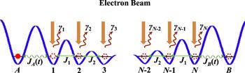
In this work we restrict our attention to transfer a single atom through a dissipative quantum data bus via tunneling passage, as illustrated in figure 1. Specifically, we consider a data bus with the simplest geometry, which is a one-dimension optical lattice of N traps by a proper choice of the barrier heights between two adjacent traps. Electron beams impacted on the traps are used to remove atom deterministically from the system. It should be noted that the dissipative lattice used here serving as data bus is to simulate an important quantum communication problem: Whether the open system can guarantee a high-fidelity QST. In our setup, the stage of the transfer procedure, the sender (trap A) and receiver (trap B) are successively coupled to the two ends of the channel in adiabatic manner. There are three practical reasons for us to propose this scenario. First, at the end of the transfer process, the atom is permanently stored in the receiving trap and will not return back into the sender due to further dynamics. Second, the adiabatic process is robust against experimental details such as the transfer time. Third, the requirements of tunneling control are minimized which allow our proposal to be implemented easily in experiments.

Figure 1.

New window|Download| PPT slide
Figure 1.Schematic illustrations of multiple-range adiabatic quantum state transfer from site A to B through an N trap optical lattice. Electron beams impacted on the traps are used to remove atom deterministically from the system. The loss rate at the lth trap is ${\gamma }_{l}$. Sender A and receiver B are time-dependently coupled to the two ends of the traps array. The neutral atom is assumed to be initialized in site A at the beginning of transport, while the other traps are empty. The atom can be transported through the lattice by adiabatically modulating J_A and J_B.


Before discussing these results, we make the following assumptions: (i) we assume N as an odd number, i.e. $N=2{N}_{0}-1$ (where N₀ is an arbitrary positive integer); however, the analysis holds for an even number of sites as well. (ii) We assume that cooling is sufficiently effective so that only the ground state of the trap potential is occupied. (iii) We assume all traps to be of the same shape and therefore the resonant tunneling takes place from one to the another one by one. In the tight-binding approximation and for open boundary conditions the Hamiltonian of the system reads(1)$\begin{eqnarray}\begin{array}{rcl}\hat{{ \mathcal H }}(t) & = & {\hat{{ \mathcal H }}}_{M}+{\hat{{ \mathcal H }}}_{C},\\ {\hat{{ \mathcal H }}}_{M} & = & \displaystyle \sum _{j=1}^{N}-{J}_{j}\left({\hat{a}}_{j}^{\dagger }{\hat{a}}_{j+1}+{\rm{h}}.{\rm{c}}.\right),\\ {\hat{{ \mathcal H }}}_{C} & = & -{J}_{A}\left(t\right){\hat{a}}_{A}^{\dagger }{\hat{a}}_{1}-{J}_{B}\left(t\right){\hat{a}}_{N}^{\dagger }{\hat{a}}_{B}+{\rm{h}}.{\rm{c}}.,\end{array}\end{eqnarray}$where ${\hat{a}}_{j}$ (${\hat{a}}_{j}^{\dagger }$) represents the annihilation (creation) operator on the j-th site, such that $\left|j\right\rangle ={\hat{a}}_{j}^{\dagger }\left|0\right\rangle ;$ J_j is the tunneling strengths between adjacent traps. J_j is controlled by the height of the barrier. The higher the barrier, the smaller the overlap between the neighboring Wannier functions and thus the smaller the tunneling strength. For definiteness in what follows, we shall assume the quantum channel is mirror symmetry, i.e. ${J}_{j}={J}_{N-j}$ $\left(j=1,2,\ldots ,\,N-1\right)$. As mentioned before, our protocol requires that trap A (controlled by the sender) and trap B (controlled by the receiver) should be time-dependently coupled to the open channel. That is to say, ${J}_{A}\left(t\right)$ and ${J}_{B}\left(t\right)$ are time-dependent, which is set in the following that(2)$\begin{eqnarray}\begin{array}{rcl}{J}_{A}\left(t\right) & = & {J}_{0}g\left(t\right),\\ {J}_{B}\left(t\right) & = & {J}_{0}g\left({t}_{\max }-t\right),\end{array}\end{eqnarray}$with $0\leqslant g\left(t\right)\leqslant 1$ for $t\in \left[0,{t}_{\max }\right]$. Here, J₀ and ${t}_{\max }$ are the peak values of the tunneling strength and time delay of the transfer process, respectively. In this paper, we choose to measure time given in units of ${J}_{0}^{-1}$. Experimentally, the time-dependent couplings ${J}_{A}\left(t\right)$ and ${J}_{B}\left(t\right)$ can be obtained by modulating the separation distance between A and j=1 trap, and B and j=N trap, respectively [20, 62].

2.2. The problem formulation and the wavefunction solutions

In this proposal, the adiabatic transport utilizes the eigenstates of equation (1) which have zero eigenvalue. We restrict our treatment to the case of having only one particle in the whole system and we write the null state as $\left|{\lambda }_{0}\left(t\right)\right\rangle ={f}_{A}\left|A\right\rangle +{\sum }_{j=1}^{N}{f}_{j}\left|l\right\rangle +{f}_{B}\left|B\right\rangle $. The probability amplitudes ${f}_{j},$ $j\in \left[1,{N}_{0}-1\right]$, can be determined by the instantaneous Hamiltonian eigenequation $\hat{{ \mathcal H }}(t)\left|{\lambda }_{0}\left(t\right)\right\rangle =0$:(3)$\begin{eqnarray}{J}_{j}{f}_{j}+{J}_{j+1}\ {f}_{j+2}=0,\end{eqnarray}$(4)$\begin{eqnarray}{f}_{N+1-2j}+{{\rm{e}}}^{{\rm{i}}{N}_{0}\pi }{f}_{2j}=0,\end{eqnarray}$and(5)$\begin{eqnarray}{J}_{A}\left(t\right){f}_{A}+{J}_{1}{f}_{2}=0,\end{eqnarray}$(6)$\begin{eqnarray}{J}_{B}\left(t\right){f}_{B}+{J}_{1}{f}_{N-1}=0.\end{eqnarray}$

First we note that all of the f_j at odd sites must vanish from equations (3)–(6) i.e. ${f}_{2j-1}=0;$ second we can write down the values of the f_j at even sites as a series, i.e.(7)$\begin{eqnarray}{f}_{2j+2}=-\displaystyle \frac{{J}_{2j}}{{J}_{2j+1}}{f}_{2j},\end{eqnarray}$and(8)$\begin{eqnarray}{J}_{B}\left(t\right){f}_{B}={J}_{A}\left(t\right){{\rm{e}}}^{{\rm{i}}\left({N}_{0}+1\right)\pi }{f}_{A}.\end{eqnarray}$Thus, $\left|{\lambda }_{0}\left(t\right)\right\rangle $ can be directly written as (unnormalized)(9)$\begin{eqnarray}\begin{array}{lll}\left|{\lambda }_{0}\left(t\right)\right. \rangle & = & {J}_{B}\left(t\right)\left|A\right. \rangle +{J}_{A}\left(t\right){{\rm{e}}}^{{\rm{i}}\left({N}_{0}+1\right)\pi }\left|B\right. \rangle -{J}_{B}\left(t\right)\displaystyle \frac{{J}_{A}\left(t\right)}{{J}_{1}}\\ & & \times \,\left\{\left|2\right. \rangle +\displaystyle \frac{1}{2}\sum _{l=2}^{{N}_{0}-1}\displaystyle \prod _{j=1}^{l-1}{\left(-1\right)}^{j}\displaystyle \frac{{J}_{2j}}{{J}_{2j+1}}\left[\left|2l \rangle \right.\right.\right.\\ & & \left.\left.+\,{{\rm{e}}}^{{\rm{i}}\left({N}_{0}+1\right)\pi }\left|N+1-2l\right. \rangle \right]+{{\rm{e}}}^{{\rm{i}}\left({N}_{0}+1\right)\pi }\left|N-1\right. \rangle \Space{0ex}{3.60ex}{0ex}\right\}.\end{array}\end{eqnarray}$It is worth mentioning that the tunneling structure of medium Hamiltonian is centrosymmetry, i.e. ${J}_{j}={J}_{N-j}$.

To realize successful state transfer of the particle across the array, one may actually require an appropriate eigenstate of the system which is free of any contribution from the leaky states $\left|j\right\rangle $ at all times. It is not difficult to see that if the condition ${J}_{0}\ll {J}_{1}\ll {J}_{2}\,\ll \cdots \ll \,{J}_{{N}_{0}}$ is held, there must exist a ‘dark state’ in the general form(10)$\begin{eqnarray}\left|{\lambda }_{0}\left(t\right)\right\rangle \approx \left|{\lambda }_{d}\left(t\right)\right\rangle =\cos \theta \left(t\right)\left|A\right\rangle +{{\rm{e}}}^{{\rm{i}}\left({N}_{0}+1\right)\pi }\sin \theta \left(t\right)\left|B\right\rangle ,\end{eqnarray}$with $\tan \theta \left(t\right)={J}_{A}\left(t\right)/{J}_{B}\left(t\right)$. Equation (10)isvery similar, in form, to the dark state in three-level system [19]. Given a total transfer time ${t}_{\max }$, our aim is to induce population transfer from state $\left|A\right\rangle $ to $\left|B\right\rangle $ by maintaining the system in null state $\left|{\lambda }_{0}\left(t\right)\right\rangle $ and changing the characteristics of $\left|{\lambda }_{0}\left(t\right)\right\rangle $ from $\left|A\right\rangle $ at t=0 to $\left|B\right\rangle $ at $t={t}_{\max }$.

It will be shown in next section that our scheme can realize a high-fidelity and long-distance QST against the particle loss effect. However, the obtained conclusion should be based on the fact that the approximate expression (10) is valid in the studied range. Such a validity of equation (10) is investigated by comparing $\left|{\lambda }_{d}\left(t\right)\right\rangle $ with the reduced state from the instantaneous eigenstate $\left|{\lambda }_{0}\left(t\right)\right\rangle $ of $\hat{{ \mathcal H }}(t)$. At half the total transfer time $t={t}_{\max }/2$, a measure of the similarity between two quantum states is given by the fidelity ${ \mathcal P }=\left\langle {\lambda }_{d}\left({t}_{\max }/2\right)\right|{\hat{\rho }}_{{AB}}\left|{\lambda }_{d}\left({t}_{\max }/2\right)\right\rangle ,$ where ${\hat{\rho }}_{{AB}}$ = Tr ${}_{M}\left(\left|{\lambda }_{0}\left({t}_{\max }/2\right)\right\rangle \left\langle {\lambda }_{0}\left({t}_{\max }/2\right)\right|\right)$ is the reduced density matrix obtained from the density matrix of the entire system by tracing out the variables of the bus. By a straightforward calculation we have(11)$\begin{eqnarray}{ \mathcal P }={\left[1+\displaystyle \frac{1}{8}\sum _{l=1}^{{N}_{0}}\prod _{j=0}^{l-1}{\left(\displaystyle \frac{{J}_{2j}}{{J}_{2j+1}}\right)}^{2}\right]}^{-1}.\end{eqnarray}$

To ensure the validity of the expression in equation (10) (${ \mathcal P }\sim 1$),the quantities ${J}_{2j}/{J}_{2j+1}$ should be small enough. While this is possible in principle it is difficult in experiment for long channel. It is worthwhile to note that the quantity ${J}_{0}/{J}_{1}$ plays a more dominant role than others. One can significantly improve the fidelity by selecting the value of ${J}_{0}/{J}_{1}$ appropriately. In particular, choosing ${J}_{0}/{J}_{1}$ small enough, the fidelity ${ \mathcal P }$ can be made arbitrarily close to unity. Thus, we can choose the interactions between the traps of the bus are uniform, i.e.${J}_{j}=J$ $\left(j=1,2,\ldots ,N-1\right)$, whereas the couplings J₀ between the boundaries of the bus and the external traps A and B are different which are smaller than J. In this case,the fidelity ${ \mathcal P }$ can be reduced to ${ \mathcal P }={\left[1+\left({N}_{0}-1\right){\left({J}_{0}/J\right)}^{2}/8\right]}^{-1}$. For instance,for N=7 traps,the fidelity is about 88.9% while choosing $J/{J}_{0}=1$.Increasing the ratio $J/{J}_{0}$ from 1 to 5 would yield the fidelity exceeding 99.5%. In order to provide the most economical choice of parameters for reaching near perfect dark state,we perform numerical analysis for different N,as shown in figure 2. Specifically,we depict the optimum quantity $J/{J}_{0}$ as a function of N for a given tolerable fidelity ${ \mathcal P }=99.5 \% $. One can see that the quantity $J/{J}_{0}$ needed to generate the high fidelity between $\left|{\lambda }_{0}\left(t\right)\right\rangle $ and $\left|{\lambda }_{d}\left(t\right)\right\rangle $ is almost linearly increased with the increase of N.

Figure 2.

New window|Download| PPT slide
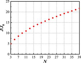
Figure 2.For a chosen fidelity ${ \mathcal P }=99.5 \% $ the optimum value of $J/{J}_{0}$ as a function of trap number N of data bus.


It is possible to mention that without dissipation, the value of fidelity ${ \mathcal P }$ provides no information on the transfer fidelity (probability of successful transfer from site A to B). However, we will show that the transfer efficiency is limited by ${ \mathcal P }$ during the transfer after taking loss factor into account.

So far, the existence of a vehicle for state transfer has been demonstrated in the context. The key idea is the engineering of increasing the tunneling strength configuration thus interactions along the chain that are able to protect state transfer against dissipation. In many physical realizations of quantum networks, the tunneling between two adjacent sites is directly related to their spatial separation. Therefore, the increasing tunneling configuration can be efficiently engineered by adjusting the site separation. The smaller the separation is, the larger the tunneling strength is.

We start our quantitative study by exploiting an alternative way of achieving complete population transfer via adiabatic evolution in closed quantum systems. It is clear from equation (10) that, to guarantee ${J}_{A}\left(0\right)/{J}_{B}\left(0\right)=0$, we should simultaneously have $\theta \left(0\right)=0$, then the state $\left|{\lambda }_{0}\left(t=0\right)\right\rangle $ is equal to $\left|A\right\rangle $. Similarly, to guarantee ${J}_{B}\left({t}_{\max }\right)/{J}_{A}\left({t}_{\max }\right)=0$, we should simultaneously have $\theta \left({t}_{\max }\right)=\pi /2$, thus the state $\left|{\lambda }_{0}\left({t}_{\max }\right)\right\rangle $ is equal to $\left|B\right\rangle $. Without dissipation, we can change the mixing angle θ from 0 into π/2 to transfer the particle from site A to B by adiabatically varying ${J}_{A}\left(t\right)$ and ${J}_{B}\left(t\right)$. In so doing, the process requires the counterintuitive pulse sequence of the tunneling strengths ${J}_{A}\left(t\right)$ and ${J}_{B}\left(t\right)$, i.e. ${J}_{B}\left(t\right)$ precedes ${J}_{A}\left(t\right)$.

2.3. Condition for adiabatic state transfer

To realize high-fidelity QST, we require that the evolution is adiabatic. During the adiabatic evolution, the system remains in its null state $\left|{\lambda }_{0}\left(t\right)\right\rangle $ at all time and there is low probability that the system will make a non-adiabatic transition to other energy eigenstates $\left|{\lambda }_{n}\left(t\right)\right\rangle $ $\left(n\ne 0\right)$. To quantify the adiabatic transfer, we introduce the adiabaticity parameter(12)$\begin{eqnarray}{{ \mathcal A }}_{n}\left(t\right)=\displaystyle \frac{\left|\ \left\langle {\dot{\lambda }}_{0}\left(t\right)\right|\left.{\lambda }_{n}\left(t\right)\right\rangle \right|}{\left|\ \left\langle {\lambda }_{0}\left(t\right)\right|\hat{{ \mathcal H }}\left|{\lambda }_{0}\left(t\right)\right\rangle -\left\langle {\lambda }_{n}\left(t\right)\right|\hat{{ \mathcal H }}\left|{\lambda }_{n}\left(t\right)\right\rangle \right|},\end{eqnarray}$where overdot denotes time differentiation. For adiabatic evolution of the system, we require ${{ \mathcal A }}_{n}\left(t\right)\ll 1$ for all $n\ne 0$. Since the adiabaticity parameter ${{ \mathcal A }}_{n}\left(t\right)$ is inversely proportional to the energy difference between the null state $\left|{\lambda }_{0}\left(t\right)\right\rangle $ and nth eigenstate $\left|{\lambda }_{n}\left(t\right)\right\rangle $. Thus it is reasonable to calculate the adiabaticity just between the null state and either of the nearest neighbors. In particular, we choose the closest positive eigenstate $\left|{\lambda }_{1}\left(t\right)\right\rangle $ to illustrate the behavior of adiabaticity ${{ \mathcal A }}_{1}\left(t\right)$ evaluated from equation (12).

As discussed before, the transfer is accomplished by applying two tunneling strengths coming in the counterintuitive sequence, i.e. ${J}_{B}\left(t\right)$ before ${J}_{A}\left(t\right)$. For simplicity, the tunnelings (2) are modulated in sinusoidal form to the second power(13)$\begin{eqnarray}g\left(t\right)={\sin }^{2}\left(\displaystyle \frac{\pi t}{2{t}_{\max }}\right),\end{eqnarray}$which are illustrated in figure 3(a).

Figure 3.

New window|Download| PPT slide
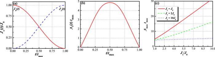
Figure 3.(a) Coupling strengths J_A and J_B as a function of time. J_A is the dashed line and J_B is the solid line. (b) Adiabaticity ${{ \mathcal A }}_{1}\left(t\right){t}_{\max }$ as a function of time t. Parameters of the calculations are $N=5,{J}_{1}={J}_{2}=10{J}_{0}$. (c) Adiabaticity ${{ \mathcal A }}_{\max }\left(t\right){t}_{\max }$ as a function of ${J}_{1}/{J}_{0}$ for N=5 and three values of J₂. The adiabaticity grows approximately linearly with coupling strength ${J}_{1}/{J}_{0}$. The bigger the J₂ is, the smaller the growth rate is.


In figure 3(b), we numerically plot the product of the adiabaticity ${{ \mathcal A }}_{1}\left(t\right)$ and the total transfer time ${t}_{\max }$ as a function of the pulse time t. Note that the greatest adiabaticity ${{ \mathcal A }}_{\max }{t}_{\max }$ occurs at the crossing point of the two pulses, which is regardless of the value of ${t}_{\max }$. This means that the larger ${t}_{\max }$, the smaller ${{ \mathcal A }}_{\max }$. For example, for N=5 and ${J}_{1}={J}_{2}=10{J}_{0}$, at $t={t}_{\max }/2$ we find ${{ \mathcal A }}_{\max }{t}_{\max }\approx \sqrt{3}\pi /{J}_{0}$. In practical applications, experience suggests the adiabatic criterion ${{ \mathcal A }}_{\max }\leqslant 0.1$. Hence the total transfer time obey the experience formula ${t}_{\max }\geqslant 10\times \sqrt{3}\pi /{J}_{0}$. With longer ${t}_{\max }$, then lower ${{ \mathcal A }}_{\max }$, the transported atom is more likely to remain in the desired $\left|{\lambda }_{0}\left(t\right)\right\rangle $ state resulting in better fidelity transfer.

We now turn our attention to calculating the maximum adiabaticity ${{ \mathcal A }}_{\max }{t}_{\max }$ for five-site quantum channel as shown in figure 3(c). It has been shown that the tunneling parameters J_j can affect the adiabaticity because they affect the energy gap between two nearest energy levels. The larger the intertrap tunneling strengths J_j are, the longer the transfer time ${t}_{\max }$ will be.

To verify above discussion, the phenomenon of coherent population transfer is investigated by numerically solving the Schrödinger equation for the density matrix $\hat{\rho }$ of the system(14)$\begin{eqnarray}\displaystyle \frac{{\rm{d}}}{{\rm{d}}t}\hat{\rho }\left(t\right)=-{\rm{i}}\left[\hat{{ \mathcal H }}\left(t\right),\hat{\rho }\left(t\right)\right].\end{eqnarray}$where we have set ℏ=1.

In the subspace of the single excitation with the basis $\left\{\left|\alpha \right\rangle ,\alpha =A,1,2,3,B\right\}$, the general density matrix is decomposed as(15)$\begin{eqnarray}\hat{\rho }=\sum _{\alpha ,\beta }{\rho }_{\alpha \beta }\left|\alpha \right\rangle \left\langle \beta \right|,\end{eqnarray}$and equation (14) is solved with initial conditions(16)$\begin{eqnarray}{\rho }_{{AA}}\left(0\right)=1,\ {\rho }_{\alpha \beta }\left(0\right)=0\ \left(\alpha \beta \ne {AA}\right).\end{eqnarray}$Our objective is to derive the populations ${\rho }_{\alpha \alpha }\left(t\right)$ which determine the occupation probability of electron in site α (α=A, 1, 2, 3, B), with normalization ${\sum }_{\alpha }{\rho }_{\alpha \alpha }\left(t\right)=1$.

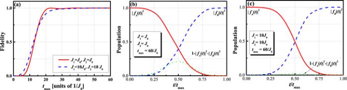
In figure 4(a) the final populations on site B,i.e. ${\rho }_{{BB}}\left({t}_{\max }\right)$, are plotted as a function of the total transfer time ${t}_{\max }$. In the absence of dissipation, ${\rho }_{{BB}}\left({t}_{\max }\right)$ increases with ${t}_{\max }$ increases, as long as adiabaticity condition is achieved. For N=5, the total transfer time ${t}_{\max }$ which is greater than $30/{J}_{0}$ can guarantee the near perfect quantum state transfer $\left({\rho }_{{BB}}\left({t}_{\max }\right)\geqslant 99 \% \right)$. In figures 4(b) and (c) we show the numerically evaluated probabilities in the three sites with the squared sinusoidal tunneling functions for J₁=J₂=J₀, and ${J}_{1}={J}_{2}=10{J}_{0}$. Here the total transfer time ${t}_{\max }$ we chosen is $60/{J}_{0}$. Figure 4 shows that 100% state transfer between the two ends of the chain can be achieved through our adiabatic process. Figure 4 also shows that the middle site occupation of particle can be suppressed with increasing the system parameters J₁ and J₂, as foreshadowed above.

Figure 4.

New window|Download| PPT slide
Figure 4.Plots of time evolution of the initial state $\left|{\rm{\Psi }}\left(t=0\right)\right\rangle =\left|A\right\rangle $. (a) The transfer fidelity as a function of total transfer time t_max for J₁=J₂=J₀ (blue dashed line), and ${J}_{1}={J}_{2}=10{J}_{0}$ (red solid line). (b) Population transfer as a function of time obtained for ${J}_{1}={J}_{2}={J}_{0}$. The red, solid curve represents the probability of $\left|A\right\rangle $ on state $\left|{\rm{\Psi }}\left(t\right)\right\rangle $. The blue, dashed curve represents the probability of $\left|B\right\rangle $ on state $\left|{\rm{\Psi }}\left(t\right)\right\rangle $. The population on medium’s sites is shown as green, dotted curve. (c) The same as in (b), but for ${J}_{1}={J}_{2}=10{J}_{0}$. Both cases could achieve 100% quantum state transfer since the adiabatic condition is satisfied. The values of the chosen parameters are shown in the figure.

3. State transfer with particle loss

3.1. The dynamics in open system

In this section, we extend the proposal of adiabatic QST discussed above from closed systems to open systems. Different from dynamical invariants in closed quantum systems, the time evolution of dynamical invariants of open quantum systems is no longer unitary. Assuming that the particles are removed rapidly and irreversibly from the dissipative traps, particle loss is described by a superoperator within the Born–Markov approximation, which reads(17)$\begin{eqnarray}{ \mathcal L }\left(\hat{\rho }\right)=\sum _{j=1}^{N}{\gamma }_{j}\left[{\hat{a}}_{j}\hat{\rho }\left(t\right){\hat{a}}_{j}^{\dagger }-\displaystyle \frac{1}{2}\left\{{\hat{a}}_{j}^{\dagger }{\hat{a}}_{j},\hat{\rho }\left(t\right)\right\}\right],\end{eqnarray}$where $\left\{\cdot ,\cdot \right\}$ denotes the anticommutator; ${\gamma }_{j}$ $\left(\geqslant 0\right)$ denotes the loss rate at site j which can be experimentally tuned by changing the strength of the applied electron beam [63–65]. For the sake of simplicity, we shall further restrict our discussion to the case ${\gamma }_{j}=\gamma $ for all j.

In general, such modification would require the formulation of a master equation instead of the Schrödinger equation. Assuming that the particles are removed rapidly and irreversibly from the lattice, the dissipative dynamics can be described by a Born–Markov approximation, which reads(18)$\begin{eqnarray}\displaystyle \frac{{\rm{d}}\hat{\rho }\left(t\right)}{{\rm{d}}t}=-{\rm{i}}\left[\hat{{ \mathcal H }}\left(t\right),\hat{\rho }\left(t\right)\right]+{ \mathcal L }\left(\hat{\rho }\right).\end{eqnarray}$For γ=0, the above equation is reduced to be Schrödinger equation (14).

Using the above equation, one can derive equations governing the evolution of the particle transfer including particle losing. We care about the effect of the particle losing on the quantum state transfer. We now derive our master equation which is the central result of this paper.

In the subspace of the single excitation plus the vacuum with the basis $\left\{\left.\left|j\right\rangle \ \right|j=A,1,2,\,\ldots ,\,N,B\right\}$, the general density matrix is decomposed into(19)$\begin{eqnarray}\hat{\rho }(t)=\sum _{j,{j}^{{\prime} }}{\rho }_{{{jj}}^{{\prime} }}(t)\left|j\right\rangle \left\langle {j}^{{\prime} }\right|.\end{eqnarray}$

Define $\left\langle N(t)\right\rangle ={\sum }_{j}{\rho }_{{jj}}$ as the expectation value of particle remains in system at time t. According to equation (18), the rate of change of $\left\langle N(t)\right\rangle $ is given by(20)$\begin{eqnarray}\displaystyle \frac{{\rm{d}}\left\langle N(t)\right\rangle }{{\rm{d}}t}=-\gamma \sum _{j=1}^{N}{\rho }_{{jj}}\left(t\right).\end{eqnarray}$The above equation can be integrated to yield(21)$\begin{eqnarray}\left\langle N({t}_{\max })\right\rangle =1-\gamma \sum _{l=1}^{N}{\int }_{0}^{{t}_{\max }}{\rho }_{{jj}}\left(t\right){\rm{d}}t,\end{eqnarray}$which suggests that the expectation value $\left\langle N(t)\right\rangle $ will not decrease while the probability of finding particle in central sites remains zero at all times. To evaluate the extent to which the dissipation affects state transfer in a open system, we adopt the concept of fidelity to completely characterize the state transfer which is from an initial state $\left|A\right\rangle $ to a target state $\left|B\right\rangle $(22)$\begin{eqnarray}{ \mathcal F }\left({t}_{\max }\right)=\mathrm{tr}\left(\hat{\rho }({t}_{\max })\left|B\right\rangle \left\langle B\right|\right).\end{eqnarray}$

3.2. Numerical results

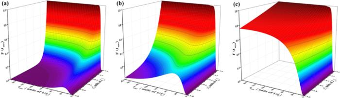
Here we discuss the dissipative effects on transfer of quantum state. We numerically integrated the master equation (18)with the same initial condition as equation (16) and the pulsing sequence equation (13). Let us consider a system of N=3 interacting dissipation modules, coupled via ${\hat{{ \mathcal H }}}_{M}$ in equation (1), depending on only one parameter J₁. In figure 5 we show the transfer fidelity ${ \mathcal F }\left({t}_{\max }\right)$ as a function of the total transfer time ${t}_{\max }$ and loss rate γ for three different values of J₁. When particle loss is added, the transfer fidelity will be reduced to some extent even if the adiabaticity condition is satisfied since particle loss from the open system cannot be recovered. For a given γ, increasing transfer time ${t}_{\max }$ can enhance the adiabaticity but reduces the transfer fidelity. There is an optimum value for ${t}_{\max }$ that maximizes the transfer fidelity ${ \mathcal F }\left({t}_{\max }\right)$. This optimal value is a balance between maximizing adiabaticity of the evolution and minimizing loss of particles. The maximum value of transfer fidelity can be improved by increasing the tunneling strengths of the quantum channel. For example, for $\gamma =0.1{J}_{0}$, the maximal transfer fidelity is 75% by setting ${J}_{1}={J}_{0}$, and can be increased to 96.5% by setting ${J}_{1}=10{J}_{0}$. This confirms that the dissipation dynamics for such open system can be suppressed efficiently by properly preparing the channel parameter J_i $\left(i=1,2,\ldots \right)$. On the other hand, the figure also indicates that the transfer fidelity decreases rapidly as the dissipative rate γ increases. But for the structure of larger (inner) tunneling strength J₁, it becomes more robust against data bus dissipation effects on the QST process. One can imagine that in the limit ${J}_{1}\gg {J}_{0}$, the transfer fidelity tends towards unity.

Figure 5.

New window|Download| PPT slide
Figure 5.Figure shows the transfer fidelity ${ \mathcal F }\left({t}_{\max }\right)$ as a function of transfer delay time ${t}_{\max }$ and loss rate $\gamma $ with N=3 dissipative modules for (a) ${J}_{1}={J}_{0}$, (b) ${J}_{1}=2{J}_{0}$, and (c) ${J}_{1}=10{J}_{0}$. The time ${t}_{\max }$ is in units of $1/{J}_{0}$ and dissipative rate $\gamma $ in units of J₀.


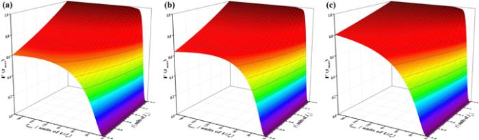
Moreover, the dissipative modules number N also bring a negative effect to the transfer fidelity. We numerically solved the master equation (18) for N=5 dissipative modules; results for the transfer fidelity as a function of transfer time ${t}_{\max }$ and loss rate γ are reported in figure 6. For tunneling strengths ${J}_{1}={J}_{2}=10{J}_{0}$ as shown in figure 6(a), one sees that the behavior of the fidelity as a function of the loss rate for N=5 decreases somewhat more rapidly than in the N=3 case (comparing figure 5(c)). When J₂ changes from 10J₀ to 50J₀, the fidelity behavior is improved close to N=3 case, see figure 6(b). Namely, more dissipative modules will lead to a faster dissipation process. In fact, this negative influence can be compensated by modulating the interaction strengths. While we choose ${J}_{1}={J}_{2}=30{J}_{0}$ (figure 6(c)), one can see that the behavior of fidelity performs better than N=3 case. As can be seen in figure 6, the values of one or both of J_1,2 are much larger than J₀. In addition, when the values of J₁ and J₂ increase at the same time, the fidelity is better than that when J₁ increases only.

Figure 6.

New window|Download| PPT slide
Figure 6.The same as in figure 4 but with N=5 dissipative modules for (a) ${J}_{1}=10{J}_{0},{J}_{2}=50{J}_{0};$ (b) ${J}_{1}=2{J}_{0},{J}_{2}=50{J}_{0};$ (c) ${J}_{1}=30{J}_{0},{J}_{2}=30{J}_{0}$.

4. Summary

Due to the fragile nature of quantum states under the influence of the decoherence environment, manipulating techniques of quantum state need to be fault tolerant to the detrimental effects of decoherence. In this paper, we have considered the adiabatic quantum state transfer through thedissipative quantum data bus, aimed at providing a feasible scheme in experiment. Firstly, we have derived an precise analytic solution to the Schr ödinger equation via Bethe ansatz and a null state (i.e. zero-eigenvalue state) is found analytically. In the limit of strong coupling between the inner traps, the null state can be approximately reduced to a coherent superposition of states $\left|A\right\rangle $ and $\left|B\right\rangle $ known as a dark state and it is this state in which particle can be adiabatically transported between two external traps A to B, without occupation of traps of data bus. We also demonstrated how to achieve higher fidelity for the dark state through optimizing the parameters of system. Then, we showed that without dissipation, the population can be perfectly transported from site A to B by slowly varying two external tunneling strengths in a counterintuitive order.

Besides providing a unitary dynamical evolution of the system, we also explore the effect of particle loss on the population dynamics in our adiabatic process. By numerically integrating the master equation, the results reveal two general conclusions: (1) there is an optimal transfer delay time for reaching the greatest transfer fidelity. The population of the final state $\left|B\right\rangle $, which is unity in the adiabatic limit in the absence of dissipation, linearly decreases as total delay time increases. (2) In the limit of strong inter-trap tunneling strengths, the leaky states will remain unpopulated during the transfer process, and the resulting particle loss effect due to leaky states is suppressed. Combining two points, one can reduce the loss by increasing the inter-trap tunnelings, either by reducing the pulse delay time ${t}_{\max }$, as long as adiabaticity is maintained.

From the experimental point of view, the open quantum channel (i.e.N traps array) can be created by superimposing two or more optical lattice differing in spatial period fields [66]. The main challenge of this work is to attain sufficient resolution to time-dependently manipulate two end traps. Recently, the single-site manipulation by an optical tweezer in a short-period optical lattice has been realized [62], which provides the possibility of overcoming this challenge.

In a word, we provide theoretical evidence that one-dimensional tight-binding array with particle loss can be used to coherently transfer particles between traps. The conclusions of the analysis are valuable for the manipulation of quantum state in solid-state systems and provide us an alternate approach, at least in principle, to tolerate the errors introduced by dissipation factor.

Acknowledgments

One of the author (BC) thanks Professor Y C Huang for helpful discussions.

Reference View Option By original order
By published year
By cited within times
By Impact factor

[1]Bose S 2003 Phys. Rev. lett. 91207901
DOI:10.1103/PhysRevLett.91.207901 [Cited within: 1]

Bose S 2007 Contemp. Phys. 48 1330
DOI:10.1103/PhysRevLett.91.207901 [Cited within: 1]

[2]Christandl M Datta N Ekert A Landahl A J 2004 Phys. Rev. Lett. 92187902
DOI:10.1103/PhysRevLett.92.187902

[3]Plenio M B Hartley J Eiser J 2004 New. J. Phys. 6 36
DOI:10.1088/1367-2630/6/1/036

[4]Song Z Sun C P 2005 Low Temp. Phys. 31 686
DOI:10.1063/1.2008129

[5]Shi T Li Y Song Z Sun C-P 2005 Phys. Rev. A 71032309
DOI:10.1103/PhysRevA.71.032309

[6]Li Y Shi T Chen B Song Z Sun C-P 2005 Phys. Rev. A 71022301
DOI:10.1103/PhysRevA.71.022301

[7]Huo M-X Li Y Song Z Sun C-P 2008 Europhys. Lett. 84 30004
DOI:10.1209/0295-5075/84/30004

[8]Whitlock S Gerritsma R Fernholz T Spreeuw R J C 2009 New. J. Phys. 11023021
DOI:10.1088/1367-2630/11/2/023021

[9]Yao N Y Jiang L Gorshkov A V Gong Z-X Zhai A Duan L-M Lukin M D 2011 Phy. Rev. Lett. 106040505
DOI:10.1103/PhysRevLett.106.040505

[10]Schlosser M Kruse J Gierl C Teichmann S Tichelmann S Birkl G 2012 New J. Phys. 14123034
DOI:10.1088/1367-2630/14/12/123034

[11]Yu S Xu P Liu M He X D Wang J Zhan M S 2014 Phys. Rev. A 90062335
DOI:10.1103/PhysRevA.90.062335

[12]Liu Y Zhou D-L 2015 New J. Phys. 17013032
DOI:10.1088/1367-2630/17/1/013032

[13]Banchi L Compagno E Bose S 2015 Phy. Rev. A 91052323
DOI:10.1103/PhysRevA.91.052323

[14]Sandberg M Knill E Kapit E Vissers M R Pappas D P 2016 Quantum Inf. Process. 15 1213
DOI:10.1007/s11128-015-1152-4

[15]Tamascelli D Olivares S Rossotti S Osellame R Paris M G A 2016 Sci. Rep. 6 26054
DOI:10.1038/srep26054

[16]de Moraes Neto G D Andrade F M Montenegro V Bose S 2016 Phys. Rev. A 93062339
DOI:10.1103/PhysRevA.93.062339

[17]Mei F Chen G Tian L Zhu S-L Jia S 2018 Phys. Rev. A 98012331
DOI:10.1103/PhysRevA.98.012331 [Cited within: 1]

[18]Bergmann K Theuer H Shore B W 1998 Rev. Mod. Phys. 70 1003
DOI:10.1103/RevModPhys.70.1003 [Cited within: 1]

[19]Greentree A D Cole J H Hamilton A R Hollenberg L C L 2004 Phys. Rev. B 70235317
DOI:10.1103/PhysRevB.70.235317 [Cited within: 2]

[20]Eckert K Lewenstein M Corbalán R Birkl G Ertmer W Mompart J 2004 Phys. Rev. A 70023606
DOI:10.1103/PhysRevA.70.023606 [Cited within: 2]

[21]Menchon-Enrich R Benseny A Ahufinger V Greentree A D Busch T Mompart J 2016 Rep. Prog. Phys. 79074401
DOI:10.1088/0034-4885/79/7/074401 [Cited within: 1]

[22]Messiah A 1961 Quantum Mechanics vol 2Amsterdam, North-Holland
[Cited within: 1]

[23]Hollenberg L C L Greentree A D Fowler A G Wellard C J 2006 Phys. Rev. B 74045311
DOI:10.1103/PhysRevB.74.045311 [Cited within: 2]

[24]Greentree A D Devitt S J Hollenberg L C L 2006 Phys. Rev. A 73032319
DOI:10.1103/PhysRevA.73.032319 [Cited within: 1]

[25]Eckert K Romero-Isart O Sanpera A 2007 New J. Phys. 9 155
DOI:10.1088/1367-2630/9/5/155 [Cited within: 1]

[26]Merkel W Mack H Freyberger M Kozlov V V Schleich W P Shore B W 2007 Phys. Rev. A 75033420
DOI:10.1103/PhysRevA.75.033420

[27]Longhi S DellaValle G Ornigotti M Laporta P 2007 Phys. Rev. B 76201101(R)
DOI:10.1103/PhysRevB.76.201101

[28]Cole J H Greentree A D Hollenberg L C L Das Sarma S 2008 Phys. Rev. B 77235418
DOI:10.1103/PhysRevB.77.235418 [Cited within: 1]

[29]Longhi S 2009 J. Mod. Opt. 59 729
DOI:10.1080/09500340802187373

[30]Jong L M Greentree A D Conrad V I Hollenberg L C L Jamieson D N 2009 Nanotechnology 20405402
DOI:10.1088/0957-4484/20/40/405402 [Cited within: 1]

[31]Rahman R Muller R P Levy J E Carroll M S Klimeck G Greentree A D Hollenberg L C L 2010 Phys. Rev. B 82155315
DOI:10.1103/PhysRevB.82.155315 [Cited within: 1]

[32]Ottaviani C Ahufinger V Corbalán R Mompart J 2010 Phys. Rev. A 81043621
DOI:10.1103/PhysRevA.81.043621 [Cited within: 1]

[33]McEndoo S Croke S Brophy J Busch T 2010 Phys. Rev. A 81043640
DOI:10.1103/PhysRevA.81.043640

[34]Benseny A Fernández-Vidal S Bagudà J Corbalán R Picón A Roso L Birkl G Mompart J 2010 Phys. Rev. A 82013604
DOI:10.1103/PhysRevA.82.013604

[35]Lubasch M Murg V Schneider U Cirac J I Bañuls M-C 2011 Phys. Rev. Lett. 107165301
DOI:10.1103/PhysRevLett.107.165301

[36]Chen B Fan W Xu Y Chen Z Y Feng X L Oh C H 2012 Phys. Rev. A 86012302
DOI:10.1103/PhysRevA.86.012302 [Cited within: 1]

[37]Wang H Liu Y-M Gao J-W Yan D Wang R Wu J-H 2012 Opt. Commun. 285 3498
DOI:10.1016/j.optcom.2012.03.013

[38]Huneke J Platero G Kohler S 2013 Phys. Rev. Lett. 110036802
DOI:10.1103/PhysRevLett.110.036802

[39]Negretti A Benseny A Mompart J Calarco T 2013 Quantum Inf. Process. 12 1439
DOI:10.1007/s11128-012-0357-z

[40]Greentree A D Koiller B 2014 Phys. Rev. A 90012319
DOI:10.1103/PhysRevA.90.012319

[41]Longhi S 2014 Ann. Phys. 348 161
DOI:10.1016/j.aop.2014.05.020 [Cited within: 1]

[42]Peng R Zheng Y Liu S-W Li X-P Wu J-L Ji X 2017 Quantum Inf. Process. 16 172
DOI:10.1007/s11128-017-1623-x

[43]Feng Z-B Lu X-J Yan R-Y Zhao Z-Y 2018 Sci. Rep. 89310
DOI:10.1038/s41598-018-27697-3 [Cited within: 1]

[44]Sarandy M S Lidar D A 2005 Phys. Rev. A 71012331
DOI:10.1103/PhysRevA.71.012331 [Cited within: 1]

Sarandy M S Lidar D A 2005 Phys. Rev. Lett. 95250503
DOI:10.1103/PhysRevA.71.012331 [Cited within: 1]

[45]Kamleitner I Cresser J Twamley J 2008 Phys. Rev. A 77032331
DOI:10.1103/PhysRevA.77.032331

[46]Hu M L 2010 Eur. Phys. J. D 59 497507
DOI:10.1140/epjd/e2010-00183-7

[47]Scala M Militello B Messina A Vitanov N V 2011 Phys. Rev. A 84023416
DOI:10.1103/PhysRevA.84.023416

[48]Witthaut D Trimborn F Hennig H Kordas G Geisel T Wimberger S 2011 Phys. Rev. A 83063608
DOI:10.1103/PhysRevA.83.063608

[49]Trimborn F Witthaut D Hennig H Kordas G Geisel T Wimberger S 2011 Eur. Phys. J. D 63 63
DOI:10.1140/epjd/e2011-10702-7

[50]Barmettler P Kollath C 2011 Phys. Rev. A 84041606
DOI:10.1103/PhysRevA.84.041606

[51]Kepesidis K V Hartmann M J 2012 Phys. Rev. A 85063620
DOI:10.1103/PhysRevA.85.063620

[52]Shchesnovich V S 2012 Phys. Rev. A 85053616
DOI:10.1103/PhysRevA.85.053616

[53]Hou Q Z Yang W L Feng M Chen C-Y 2013 Phys. Rev. A 88013807
DOI:10.1103/PhysRevA.88.013807

[54]Liu H-B An J-H Chen C Tong Q-J Luo H-G Oh C H 2013 Phys. Rev. A 87052139
DOI:10.1103/PhysRevA.87.052139

[55]Pudlik T Hennig H Witthaut D Campbell D K 2013 Phys. Rev. A 88063606
DOI:10.1103/PhysRevA.88.063606

[56]Kordas G Wimberger S Witthaut D 2013 Phys. Rev. A 87043618
DOI:10.1103/PhysRevA.87.043618

[57]Ferraro E De Michielis M Fanciulli M Prati E 2015 Phys. Rev. B 91075435
DOI:10.1103/PhysRevB.91.075435

[58]Campbell R Oppo G-L 2016 Phys. Rev. A 94043626
DOI:10.1103/PhysRevA.94.043626

[59]Overbeck V R Weimer H 2016 Phys. Rev. A 93012106
DOI:10.1103/PhysRevA.93.012106 [Cited within: 1]

[60]Ji Y Ke Q Hu J 2018 Optik 157 306
DOI:10.1016/j.ijleo.2017.11.082 [Cited within: 1]

[61]Breuer H-P Petruccione F 2002 The Theory of Open Quantum SystemsOxfordOxford University Press
[Cited within: 1]

[62]Thompson J D Tiecke T G de Leon N P Feist J Akimov A V Gullans M Zibrov A S Vuletić V Lukin M D 2013 Science 340 1202
DOI:10.1126/science.1237125 [Cited within: 2]

[63]Barontini G Labouvie R Stubenrauch F Vogler A Guarrera V Ott H 2013 Phys. Rev. Lett. 110035302
DOI:10.1103/PhysRevLett.110.035302 [Cited within: 1]

[64]Gericke T Würtz P Reitz D Langen T Ott H 2008 Nat. Phys. 4 949
DOI:10.1038/nphys1102

[65]Würtz P Langen T Gericke T Koglbauer A Ott H 2009 Phys. Rev. Lett. 103080404
DOI:10.1103/PhysRevLett.103.080404 [Cited within: 1]

[66]Föling S Trotzky S Cheinet P Feld M Saers R Widera A Müller T Bloch I 2009 Nature 448 10291032
DOI:10.1038/nature06112 [Cited within: 1]