Shao-Fu He(何少甫)^1,2, Yang Wang(汪洋)^,1,2,3, Jia-Ji Li(李家骥)^1,2, Wan-Su Bao(鲍皖苏)^,1,2,31Henan Key Laboratory of Quantum Information and Cryptography, SSF IEU, Zhengzhou, Henan 450001, China
²Synergetic Innovation Center of Quantum Information and Quantum Physics, University of Science and Technology of China, Hefei, Anhui 230026, China

First author contact: ³Authors to whom any correspondence should be addressed.
Received:2020-01-3Revised:2020-03-12Accepted:2020-03-18Online:2020-05-18


Abstract
Twin-field quantum key distribution (TF-QKD) is a disruptive innovation which is able to overcome the rate-distance limit of QKD without trusted relays. Since the proposal of the first TF-QKD protocol, theoretical and experimental breakthroughs have been made to enhance its ability. However, there still exist some practical issues waiting for settlement. In this paper, we examine the performances of asymmetric TF-QKD protocol with unstable light sources and limited data sizes. The statistical fluctuations of the parameters are estimated employing Azuma’s inequality. Through numerical simulations, we compare the secret key rates of the asymmetric TF-QKD protocol with different data sizes and variant intensity fluctuation magnitudes. Our results demonstrate that both statistical and intensity fluctuations have significant impacts on the performance of asymmetric TF-QKD.
Keywords： twin-field quantum key distribution;asymmetrical losses;statistical fluctuations;intensity fluctuations


PDF (513KB)MetadataMetricsRelated articlesExportEndNote|Ris|BibtexFavorite
Cite this article
Shao-Fu He(何少甫), Yang Wang(汪洋), Jia-Ji Li(李家骥), Wan-Su Bao(鲍皖苏). Asymmetric twin-field quantum key distribution with both statistical and intensity fluctuations. Communications in Theoretical Physics, 2020, 72(6): 065103- doi:10.1088/1572-9494/ab8a11

1. Introduction

The past few decades have witnessed the rapid development of quantum key distribution (QKD) [1]. In this fast-evolving information era, the security of communication is crucial in many scenarios. QKD, whose security is guaranteed by quantum mechanics, provides a reliable platform for two remote users to share secret keys [2, 3]. However, there still remains some practical issues to be handled before the vast application of commercial QKD systems. Among these issues, the point-to-point rate-distance limit of QKD [4, 5] severely restricts the communication distance between legitimate parties. The quantum repeater scheme [6–8] was conjectured to be a perfect solution to this frustrating problem. Unfortunately, current technologies cannot meet the requirement of implementing quantum repeaters experimentally.

To overcome the fundamental rate-distance limit of QKD with current quantum communication systems, Lucamarini et al proposed the prospective TF-QKD protocol [9]. The unprecedented TF-QKD protocol enables remote legitimate users to perform secure communications without the restriction of the repeaterless bound. As a similar type of the measurement-device-independent (MDI)-QKD [10, 11], TF-QKD possesses the biggest advantage of MDI-QKD which is the security against attacks on the measurement devices. The secret key rate of TF-QKD scales with the square-root of the channel transmittance η due to the single-photon interference at the untrusted central node. Since the establishment of the original TF-QKD protocol, several variations of TF-QKD type protocols [12–18] and some of their improved versions [19, 20] have been proposed to offer more rigorous security proofs with higher performances. Subsequently, experimental investigations [21–24] are carried out to estimate the practicality of TF-QKD and the results are satisfactory. However, there still exists an inevitable gap between TF-QKD protocols and commercial QKD implementations at present. Recently, several works [25–30] have been done to study the finite-key effect of variant TF-QKD protocols. Moreover, the security of TF-QKD with intensity fluctuations is also examined in [31]. Apart from finite-key effect and intensity fluctuations, protocols with asymmetric losses [32–35] are proposed to test the ability of asymmetrical TF-QKD extensively.

Here, we focus on the asymmetric TF-QKD protocol proposed by Grasselli et al [33]. Developed from the TF-QKD protocol proposed by Curty et al [17], this asymmetric TF-QKD maintains the strengths of the original protocol such as high secret key rate and robustness against phase misalignments. Moreover, this asymmetric TF-QKD protocol is proved to be effective with both decoy-state methods [36–38] and asymmetrical losses. Nonetheless, the secret key rate of the asymmetric TF-QKD protocol is estimated with infinite signal pulses which is infeasible in practical systems [39, 40]. Furthermore, in real-life quantum communication setups, the intensities of the signal pulses are not always steady which would possibly undermine the security of TF-QKD [41–44].

In this paper, we investigate the performance of the asymmetric TF-QKD protocol with finite-key effect and unstable sources cohesively. Here, we provide the modified asymmetric TF-QKD protocol in finite-key regime with intensity fluctuations taken into account. The statistical fluctuations of the parameters are estimated by Azuma’s inequality [45, 46]. With the linear channel loss model, we numerically simulated the secret key rate of the modified asymmetric TF-QKD protocol in the existence of both statistical and intensity fluctuations. Our numerical results demonstrate that both statistical and intensity fluctuations have ineligible influences on the asymmetrical TF-QKD.

This paper is organized as follows. After the above introduction, we provide the actual form of the asymmetric TF-QKD protocol in section 2. In section 3, we demonstrate the parameter estimation methods of the modified protocol. Then, the numerical simulation results of the final key rates are presented in section 4. Finally, we provide a conclusion of our paper in section 5.

2. Protocol description

Here we focus on an asymmetric TF-QKD protocol [33], in which a three-decoy-state method is utilized to estimate the phase error rate of the raw keys. Considering limited signal pulses, we provide the details of this protocol in finite-key regime while the light sources located in both sides are unstable. The legitimate users Alice and Bob are able to extract an identical secret key string after performing the following steps.

2.1. Preparation

At the beginning of this step, Alice and Bob are supposed to choose Z-basis or X-basis for their signal pulses. If Alice (Bob) choose Z-basis with probability ${P}_{{\rm{A}}}^{Z}$ (${P}_{{\rm{B}}}^{Z}$), she (he) prepares a coherent state pulse $\left|\sqrt{{\alpha }_{Z}}{{\rm{e}}}^{{\rm{i}}\pi {b}_{{\rm{A}}}}\right\rangle $ ($\left|\sqrt{{\beta }_{Z}}{{\rm{e}}}^{{\rm{i}}\pi {b}_{{\rm{B}}}}\right\rangle $) as a signal state, where ${\alpha }_{Z}$ (${\beta }_{Z}$) is the intensity of Alice’s (Bob’s) signal state pulse, b_A (b_B) denotes the random bit selected from the set $\left\{0,1\right\}$. If X-basis is chosen with probability $1-{P}_{{\rm{A}}}^{Z}$ ($1-{P}_{{\rm{B}}}^{Z}$), Alice (Bob) emits a phase randomized coherent state as a decoy state whose average intensity is chosen from the set ${\alpha }_{a}\in \left\{{\alpha }_{0},{\alpha }_{1},{\alpha }_{2}\right\}$ (${\beta }_{b}\in \left\{{\beta }_{0},{\beta }_{1},{\beta }_{2}\right\}$) with probabilities P_a (P_b), where $a,b\in \left\{0,1,2\right\}$ . However, the photon sources are unstable. As a result, the intensities of both signal and decoy states are fluctuating around their average values.

2.2. Measurement

After the preparation step, the signal pulses are sent to an untrusted central node Charlie through quantum channels. The channel transmittances from Alice to Charlie and Bob to Charlie are denoted as ${\eta }_{{\rm{A}}}$ and ${\eta }_{{\rm{B}}}$. Charlie is supposed to perform the measurements using a beamsplitter with two threshold detectors L and R. At this moment, the untrusted third party Charlie has no information whether the signal pulse is a signal state or a decoy state. Then, Charlie announces the output of the two detectors.

2.3. Sifting

The first two steps are supposed to be repeated for N rounds by the two legitimate parties. Here, the measurement results corresponding to only one of the two detectors clicks are called successful detection events. After that, Alice and Bob announce their choices of the basis and intensities to each other through an authenticated public channel. The successful detection events corresponding to the same basic choices are maintained for the following steps.

2.4. Parameter estimation

The total amount of Z-basis and X-basis successful detection events are denoted as s_Z and s_X. According to the decoy state intensities α_a and β_b they have chosen, Alice and Bob are able to obtain the detailed amount of s_ab of the X-basis successful detection events. Particularly, the random bits b_A and b_B of the Z-basis successful detection events are utilized to extract the final key. In our protocol, Bob always flips his bit b_B for an R detector click. Importantly, the total amount of successful detection events are exploited to estimate the phase error rate e_ph.

2.5. Postprocessing

In this step, Alice firstly sends Bob leak_EC bits to perform error correction using an information reconciliation scheme. Next, Alice exploits $\mathrm{log}\left(1/{\varepsilon }_{\mathrm{cor}}\right)$ bits to compute a hash of her raw key string. Then the hash and the random two-universal hash function are sent to Bob through the authenticated public channel. Bob computes the hash of his string to ensure that their key bits are identical. Finally, Alice and Bob utilize a random two-universal hash function to perform privacy amplification. After that, they are able to obtain two key strings K_A and K_B with secret key length L.

3. Methods

Before we demonstrate the parameter estimation methods, it is necessary to characterize the security of the protocol at first. Here, the universally composable framework is utilized in this section [30, 47, 48]. The security of a QKD protocol can be ensured by two criterions ‘correctness’ and ‘secrecy’. For two small errors ${\varepsilon }_{\mathrm{cor}}$ and ϵ_sec, the protocol is ϵ_cor-correct and ϵ_sec-secret if the following two conditions are satisfied: (1) $\Pr \left[{K}_{{\rm{A}}}\ne {K}_{{\rm{B}}}\right]\leqslant {\varepsilon }_{\mathrm{cor}}$. (2) $\tfrac{1}{2}{\parallel {\rho }_{{K}_{{\rm{A}}}{\rm{E}}}-{U}_{{K}_{{\rm{A}}}}\otimes {\rho }_{{\rm{E}}}\parallel }_{1}\leqslant {\varepsilon }_{\sec }$. Notably, ${\parallel \cdot \parallel }_{1}$ is the trace norm and ${\rho }_{{K}_{{\rm{A}}}{\rm{E}}}$ is the joint state of Alice and Eve. ${U}_{{K}_{{\rm{A}}}}$ is the mixed state of all possible values of ${K}_{{\rm{A}}}$ while ${U}_{{K}_{{\rm{A}}}}\otimes {\rho }_{{\rm{E}}}$ describes the ideal case. A QKD protocol can be described as ϵ-secure if it is both ϵ_cor-correct and ϵ_sec-secret with $\varepsilon ={\varepsilon }_{\mathrm{cor}}+{\varepsilon }_{\sec }$.

In our parameter estimation, the effect of statistical fluctuations and intensity fluctuations are taken into account concurrently. As mentioned in the above section, the total amounts of successful detection events s_Z, s_X as well as s_ab are directly observed by Alice and Bob. With these successful detection events acquired in the real protocol, the two users are able to estimate the secret key rate employing our methods.

At the beginning of our methods, we need to estimate the effect of statistical fluctuations. Although we can directly obtain the observed values of ${s}_{{ab}}$ in real experiments, the expectation values of these successful detection events are remained unknown. In the case with stable sources, the malicious eavesdropper Eve cannot acquire the intensity choices of the signal pulses due to the decoy-state method. Therefore, we can assume that the trials are independent with each other and every detection event can be regarded as an independent random variable. In this case, finite-key analysis tools such as Chernoff bound [49] and Hoeffding’s inequality [50] can be utilized to estimate the statistical fluctuations of successful detection events. Unfortunately, considering the existence of unstable sources, the eavesdropper Eve can carry out a coherent attack strategy. Eve first make all the pulses interact coherently with an auxiliary system, then she utilizes the information Alice and Bob announced in the sifting step to measure the auxiliary. Thus, the prerequisite that the detection events are independent random variables is not satisfied and both Chernoff bound [49] and Hoeffding’s inequality [50] are invalid then. In order to estimate the finite-key effect of the asymmetric TF-QKD with unstable sources, we utilize Azuma’s inequality [45, 46] which is suitable for a sequence of dependent random variables which can be correlated in anyway if the sequence is a martingale and satisfies the bounded difference condition.

Let n₀, n₁, ⋯, n_N be a sequence of random variables, the two conditions martingale and bounded difference condition can be expressed as follows:

(i) Martingale. If and only if the expectation value of ${n}_{i+1}$ conditioned on the first i+1 outcomes of n₀, n₁, ⋯, n_i satisfies $E\left[{n}_{i+1}| {n}_{0},{n}_{1},\cdots ,\,{n}_{i}\right]={n}_{i}$ for all non-negative integer i, the sequence can be regarded as a martingale.

(ii) Bounded difference condition. The bounded difference condition is satisfied if there exists ${c}_{i}\gt 0$ such that $\left|{n}_{i+1}-{n}_{i}\right|\leqslant {c}_{i}$ for all non-negative integer i.

For the sequence n₀, n₁, ⋯, n_N which contains N+1 trials and satisfies the above conditions with c_i=1, n_N can be bounded by Azuma’s inequality [45, 46](1)$\begin{eqnarray}\Pr \left[\left|{n}_{N}-{n}_{0}\right|\gt N\delta \right]\leqslant 2{{\rm{e}}}^{-N{\delta }^{2}/2}.\end{eqnarray}$

In order to apply Azuma’s inequality to our protocol, we first set m₀, m₁, ⋯ , m_N as N+1 random but dependent variables that satisfies ${m}_{j}\in \left\{0,1\right\}$. Then we denote ${s}_{i}={\sum }_{j=1}^{i}{m}_{j}$ as the observed value and ${s}_{i}^{* }={\sum }_{j=1}^{i}P\left({m}_{j}| {m}_{0},{m}_{1},\cdots ,\,{m}_{j-1}\right)$ as the expectation value of m₁, ⋯ , m_i respectively. Next, we define the ith trial of the sequence n₀, n₁, ⋯, n_N as(2)$\begin{eqnarray}\begin{array}{c}{n}_{i}=\left\{\begin{array}{ll}{s}_{i}-{s}_{i}^{\ast }+{m}_{0} & {\rm{if}}\,i\gt 0\\ {m}_{0} & {\rm{if}}\,i=0\end{array}\right..\end{array}\end{eqnarray}$We notice that the expectation value of ${n}_{i+1}$ conditioned on n₀, n₁, ⋯, n_i is exactly n_i, and $\left|{n}_{i+1}-{n}_{i}\right|\leqslant 1$ is always satisfied. Thus, this sequence n₀, n₁, ⋯, n_N is a martingale and satisfies the bounded difference condition with c_i=1. Then by employing Azuma’s inequality [45, 46], we can obtain(3)$\begin{eqnarray}\Pr \left[\left|{s}_{N}-{s}_{N}^{* }\right|\gt N\delta \right]\leqslant 2{{\rm{e}}}^{-N{\delta }^{2}/2}\end{eqnarray}$for $\delta \in \left(0,1\right)$.

In the modified asymmetric TF-QKD protocol, every detection event can be regarded as a random variable, the total trials can be regarded as a sequence with N random variables. The successful detection event s_ab can be regarded as an observed output of the sequence. We denote ${s}_{{ab}}^{* }$ as the expectation value of the sequence. Then s_N and ${s}_{N}^{* }$ in equation (3) can be replaced by s_ab and ${s}_{{ab}}^{* }$. Thus we can utilize Azuma’s inequality to rewrite equation (3) as(4)$\begin{eqnarray}{s}_{{ab}}-\sqrt{2N\mathrm{ln}\left(1/{\varepsilon }_{A}\right)}\leqslant {s}_{{ab}}^{* }\leqslant {s}_{{ab}}+\sqrt{2N\mathrm{ln}\left(1/{\hat{\varepsilon }}_{A}\right)}\end{eqnarray}$with failure probability ${\varepsilon }_{A}+{\hat{\varepsilon }}_{A}$.

In the modified asymmetric TF-QKD protocol, the expectation values ${s}_{{ab}}^{* }$ can be utilized to estimate the yields of the X-basis with(5)$\begin{eqnarray}{s}_{{ab}}^{* }=\left(1-{P}_{{\rm{A}}}^{Z}\right)\left(1-{P}_{{\rm{B}}}^{Z}\right)N\sum _{n,m}{P}_{a}{P}_{b}{P}_{n| a}{P}_{m| b}{Y}_{{nm}},\end{eqnarray}$where Y_nm is the yield that Alice and Bob send n and m photons in the X-basis respectively. The Poisson distributions of α_a and β_b can be obtained by ${P}_{n| a}={{\rm{e}}}^{-{\alpha }_{a}}{\alpha }_{a}^{n}/n!$ and ${P}_{m| b}={{\rm{e}}}^{-{\beta }_{b}}{\beta }_{b}^{m}/m!$.

Consequently, one can utilize the observed values s_ab together with Azuma’s inequality to rewrite equation (5) as(6)$\begin{eqnarray}\begin{array}{l}{s}_{{ab}}-\sqrt{2N\mathrm{ln}\left(1/{\varepsilon }_{A}\right)}\leqslant \left(1-{P}_{{\rm{A}}}^{Z}\right)\left(1-{P}_{{\rm{B}}}^{Z}\right)N\\ \times \,\sum _{n,m}{P}_{a}{P}_{b}{P}_{n| a}{P}_{m| b}{Y}_{{nm}}\leqslant {s}_{{ab}}+\sqrt{2N\mathrm{ln}\left(1/{\hat{\varepsilon }}_{A}\right)}.\end{array}\end{eqnarray}$

After that, we have obtained the expectation value of the successful detection events ${s}_{{ab}}^{* }$ with statistical fluctuations taken into account. However, intensity fluctuations not only affect the correlation between detection events, but also change the actual value of the intensities. In our protocol with unstable sources, we suppose that the largest intensity fluctuation magnitudes of the photon pulses emitted by Alice and Bob are δ_A and δ_B separately. Then we can acquire the upper bound and lower bound of the intensities of their signal states and decoy states by(7)$\begin{eqnarray}\left\{\begin{array}{l}{\alpha }_{Z}\left(1-{\delta }_{{\rm{A}}}\right)\leqslant {\alpha }_{Z}\leqslant {\alpha }_{Z}\left(1+{\delta }_{{\rm{A}}}\right)\\ {\alpha }_{a}\left(1-{\delta }_{{\rm{A}}}\right)\leqslant {\alpha }_{a}\leqslant {\alpha }_{a}\left(1+{\delta }_{{\rm{A}}}\right)\end{array}\right.,\end{eqnarray}$(8)$\begin{eqnarray}\left\{\begin{array}{l}{\beta }_{Z}\left(1-{\delta }_{{\rm{B}}}\right)\leqslant {\beta }_{Z}\leqslant {\beta }_{Z}\left(1+{\delta }_{{\rm{B}}}\right)\\ {\beta }_{b}\left(1-{\delta }_{{\rm{B}}}\right)\leqslant {\beta }_{b}\leqslant {\beta }_{b}\left(1+{\delta }_{{\rm{B}}}\right)\end{array}\right..\end{eqnarray}$In order to tightly bound the secret key rate, we consider the worst case of the secret key rate by numerically optimizing the phase error rate $\overline{{e}_{\mathrm{ph}}}$ over the all the possible intensities within the fluctuation ranges. Through substituting the intensities which we used to estimate the phase error rate by their upper bounds ($\overline{{\alpha }_{Z}}$, $\overline{{\alpha }_{a}}$, $\overline{{\beta }_{Z}}$ and $\overline{{\beta }_{b}}$) or lower bounds ($\underline{{\alpha }_{Z}}$, $\underline{{\alpha }_{a}}$, $\underline{{\beta }_{Z}}$ and $\underline{{\beta }_{b}}$), we can acquire the maximum value of the phase error rate $\overline{{e}_{\mathrm{ph}}}$. According to the original asymmetric TF-QKD protocol proposed in [33], the upper bound of phase error rate e_ph can be given by(9)$\begin{eqnarray}\begin{array}{l}\overline{{e}_{\mathrm{ph}}}=\left[{\left(\sum _{n=0,m=0}^{\infty }\overline{{M}_{2n,2m}}\sqrt{\overline{{Y}_{2n,2m}}}\right)}^{2}\right.\\ \left.+\,{\left(\sum _{n=0,m=0}^{\infty }\overline{{M}_{2n+\mathrm{1,2}m+1}}\sqrt{\overline{{Y}_{2n+\mathrm{1,2}m+1}}}\right)}^{2}\right]{{NP}}_{{\rm{A}}}^{Z}{P}_{{\rm{B}}}^{Z}/{s}_{Z},\end{array}\end{eqnarray}$where(10)$\begin{eqnarray}\overline{{M}_{{nm}}}=\displaystyle \frac{{{\rm{e}}}^{-\underline{{\alpha }_{Z}}/2-\underline{{\beta }_{Z}}/2}{\overline{{\alpha }_{Z}}}^{n/2}{\overline{{\beta }_{Z}}}^{m/2}}{\sqrt{n!m!}}.\end{eqnarray}$In our modified asymmetric TF-QKD protocol, we only estimate the upper bounds of ${Y}_{00}$, Y₀₂, Y₂₀, Y₀₄, Y₄₀, Y₂₂, Y₁₃, Y₃₁ and Y₁₁ with equation (6) and the decoy state method proposed in [33]. The other yields are replaced by the maximum value 1 for simplicity. In this way, the upper bound of the phase error rate can be obtained.

Now we have obtained the upper bound of the phase error rate with our parameter estimation methods. On the other hand, the bit error rate e_bit of the raw key bits can be directly obtained by Alice and Bob in the error correction step. Finally, according to [30], the ultimate secret key length can be given by(11)$\begin{eqnarray}L\leqslant {s}_{Z}[1-h(\overline{{e}_{\mathrm{ph}}})]-{\mathrm{leak}}_{\mathrm{EC}}-2{\mathrm{log}}_{2}\displaystyle \frac{13}{2{\varepsilon }_{\sec }}-{\mathrm{log}}_{2}\displaystyle \frac{2}{{\varepsilon }_{\mathrm{cor}}},\end{eqnarray}$where $h(x)=-x{\mathrm{log}}_{2}x-(1-x){\mathrm{log}}_{2}(1-x)$ is the binary Shannon entropy function, the amount of bits Alice and Bob sacrificed in error correction step is ${\mathrm{leak}}_{\mathrm{EC}}={s}_{Z}{fh}\left({e}_{\mathrm{bit}}\right)$ with f being the error correction inefficiency.

4. Simulations

In this section, we numerically simulate the performance of the asymmetric TF-QKD protocol with both statistical and intensity fluctuations. The secret key rate of the protocol can be obtained by R=L/N with the secret key length L estimated above. The linear channel loss model of asymmetric TF-QKD presented in [33] is adopted to simulate the observed values which can be measured in real experiments by the communication parties. In our simulations, the dark count rate and the error correction inefficiency are fixed to ${P}_{d}={10}^{-8}$ and f=1.1 respectively.

To compare the performance of the modified asymmetric TF-QKD protocol under different circumstances, we plot the secret key rate as a function of the overall loss between Alice and Bob which is measured in dB. The intensities of the signal-states are optimized over the asymmetrical losses while the intensities of the decoy-states are set to ${\alpha }_{0}={\beta }_{0}=0.5$, ${\alpha }_{1}={\beta }_{1}={10}^{-2}$ and ${\alpha }_{2}={\beta }_{2}={10}^{-4}$ for Alice and Bob. For convenience, the magnitudes that we utilized to characterize the phase and polarization misalignments are set to 2%. In addition, the PLOB bound [5] is exploited as the yardstick when describing the performances of the secret key rates. Moreover, we fix the security bounds to ${\varepsilon }_{\sec }={10}^{-10}$ and ${\varepsilon }_{\mathrm{cor}}={10}^{-15}$.

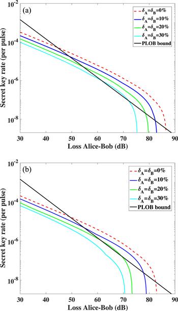
In figure 1, we demonstrate the effect of intensity fluctuations with both symmetrical and asymmetrical losses. In the case with symmetrical losses, the secret key rate is robust against intensity fluctuations. As shown in figure 1(a), the symmetric TF-QKD protocol can beat the PLOB bound with all three intensity fluctuation magnitudes. However, the secret key rate of the asymmetric TF-QKD protocol is much lower comparing with the former case. Figure 1(b) demonstrates that the protocol can hardly beat the PLOB bound when the intensity fluctuation magnitudes of Alice and Bob are larger than 20%.

Figure 1.

New window|Download| PPT slide
Figure 1.Secret key rate as a function of the overall loss between Alice and Bob with symmetrical and asymmetrical losses. (a) The loss between Alice and Charlie is the same as Bob’s side. (b) The loss between Alice and Charlie is always 10 dB larger than the loss between Bob and Charlie. The total amount of signal pulses are set to $N={10}^{14}$. In both (a) and (b), the intensity fluctuation magnitudes of Alice’s and Bob’s photon sources are set to 30%, 20% and 10% (curves from left to right). The dashed line characterizes the case with no intensity fluctuations.


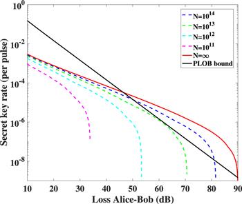
In order to study the finite-key effect with unstable sources, we compare the performances of the protocol with different amount of total signal pulses. Here, four different total amounts of signal pulses are utilized to estimate the secret key rates. As shown in figure 2, statistical fluctuations have an extremely significant impact on the secret key rate when the photon sources are unstable. In this case, the protocol cannot overcome the PLOB bound if the total signal pulses are limited. Thus, we have to ensure that the two parties emit enough signal pulses in long distance communications.

Figure 2.

New window|Download| PPT slide
Figure 2.Secret key rate in logarithmic scale as a function of the overall loss between Alice and Bob with different amount of total signal pulses. In this plot, the loss between Alice and Charlie is always 5 dB larger than the loss between Bob and Charlie. The intensity fluctuation magnitudes of Alice’s and Bob’s photon sources are set to 10%. The aggregate amount of photon pulses are set to ${10}^{11}$, ${10}^{12}$, ${10}^{13}$ and ${10}^{14}$ (dashed curves from left to right). The solid curve represents the case with infinite signal pulses.


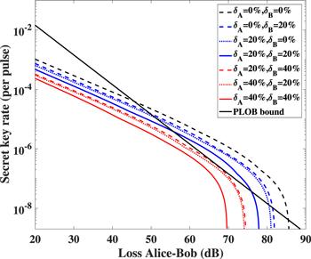
Additionally, we compare the secret key rate when the intensity fluctuation magnitudes of Alice’s and Bob’s photon sources are different. We first set the intensity fluctuation magnitudes to ${\delta }_{{\rm{A}}}=40 \% $ (${\delta }_{{\rm{B}}}=20 \% $) and ${\delta }_{{\rm{A}}}=20 \% $ (${\delta }_{{\rm{B}}}=0 \% $) as the dotted lines from left to right in figure 3. Then we exchange the intensity fluctuation magnitudes of Alice and Bob with ${\delta }_{{\rm{A}}}=20 \% $ (${\delta }_{{\rm{B}}}=40 \% $) and ${\delta }_{{\rm{A}}}=0 \% $ (${\delta }_{{\rm{B}}}=20 \% $). The results are characterized by the dashed lines close to the dotted lines. As shown in figure 3, the effects of intensity fluctuations of Alice’s and Bob’s are not the identical in the asymmetrical case.

Figure 3.

New window|Download| PPT slide
Figure 3.Secret key rate in logarithmic scale as a function of the overall loss between Alice and Bob with asymmetrical intensity fluctuation magnitudes. The dashed line on the far right represents the case with no intensity fluctuations. The total amount of signal pulses are set to N=10¹⁴ while the loss of Alice–Charlie is always 5 dB larger than Bob–Charlie.


Our simulation results suggest that the asymmetric TF-QKD protocol is still capable to beat the repeaterless bound with statistical and intensity fluctuations. However, the effects can be very significant if the data size is small. Thus, in order to obtain higher secret key rates in long-distance communications, the legitimate users are supposed to send adequate signal pulses and exploit photon sources with lower intensity fluctuation magnitudes.

5. Conclusion

In this paper, we have analyzed the asymmetric TF-QKD protocol with both statistical and intensity fluctuations. We proposed the modified asymmetric TF-QKD protocol with finite signal pulses and unstable sources. In order to estimate the statistical fluctuations, we utilized Azuma’s inequality to obtain the upper and lower bounds of the observed successful detection events. The secret key rate is obtained by numerically optimizing the phase error rate over all possible intensities. Furthermore, we simulated the performance of the protocol with finite-key length and fluctuating intensities. The simulation results indicate that statistical and intensity fluctuations cannot be neglected in asymmetric TF-QKD especially with long communication distances. In summary, our results in this paper could provide a theoretical reference for the future applications of TF-QKD.

Acknowledgments

Project supported by National Natural Science Foundation of China (61675235, 61605248 and 61505261) and National Key Research and Development Program of China (2016YFA0302600).

Reference View Option By original order
By published year
By cited within times
By Impact factor

[1]Bennett C H Brassard G 1984Proc. IEEE Int. Conf. on Computers, Systems and Signal ProcessingBangalore, IndiaNew YorkIEEE175179
[Cited within: 1]

[2]Lo H K Curty M Tamaki K 2014 Nat. Photon. 8 595604
DOI:10.1038/nphoton.2014.149 [Cited within: 1]

[3]Scarani V Bechmann-Pasquinucci H Cerf N J Dusek M Lütkenhaus N Peev M 2009 Rev. Mod. Phys. 81 13011350
DOI:10.1103/RevModPhys.81.1301 [Cited within: 1]

[4]Takeoka M Guha S Wilde M M 2014 Nat. Commun. 5 5235
DOI:10.1038/ncomms6235 [Cited within: 1]

[5]Pirandola S Laurenza R Ottaviani C Banchi L 2017 Nat. Commun. 8 15043
DOI:10.1038/ncomms15043 [Cited within: 2]

[6]Briegel H J Dür W Cirac J I Zoller P 1998 Phys. Rev. Lett. 81 5932
DOI:10.1103/PhysRevLett.81.5932 [Cited within: 1]

[7]Duan L M Lukin M D Cirac J I Zoller P 2001 Nature 414 413418
DOI:10.1038/35106500

[8]Sangouard N Simon C de Riedmatten H Gisin N 2011 Rev. Mod. Phys. 83 3380
DOI:10.1103/RevModPhys.83.33 [Cited within: 1]

[9]Lucamarini M Yuan Z L Dynes J F Shields A J 2018 Nature 557 400
DOI:10.1038/s41586-018-0066-6 [Cited within: 1]

[10]Braunstein S L Pirandola S 2012 Phys. Rev. Lett. 108130502
DOI:10.1103/PhysRevLett.108.130502 [Cited within: 1]

[11]Lo H K Curty M Qi B 2012 Phys. Rev. Lett. 108130503
DOI:10.1103/PhysRevLett.108.130503 [Cited within: 1]

[12]Wang X B Yu Z W Hu X L 2018 Phys. Rev. A 98062323
DOI:10.1103/PhysRevA.98.062323 [Cited within: 1]

[13]Ma X F Zeng P Zhou H Y 2018 Phys. Rev. X 8031043
DOI:10.1103/PhysRevX.8.031043

[14]Tamaki K Lo H K Wang W Lucamarini M 2018arXiv:1805.05511


[15]Cui C Yin Z Q Wang R Chen W Wang S Guo G C Han Z F 2019 Phys. Rev. Appl. 11034053
DOI:10.1103/PhysRevApplied.11.034053

[16]Curty M Azuma K Lo H K 2019 NPJ Quantum Inf. 5 64
DOI:10.1038/s41534-019-0175-6

[17]Lin J Lütkenhaus N 2018 Phys. Rev. A 98042332
DOI:10.1103/PhysRevA.98.042332 [Cited within: 1]

[18]Yin H L Fu Y 2019 Sci. Rep. 9 3045
DOI:10.1038/s41598-019-39454-1 [Cited within: 1]

[19]Lu F Y et al. 2019 Phys. Rev. A 100022306
DOI:10.1103/PhysRevA.100.022306 [Cited within: 1]

[20]Grasselli F Curty M 2019 New J. Phys. 21073001
DOI:10.1088/1367-2630/ab2b00 [Cited within: 1]

[21]Minder M Pittaluga M Roberts G L Lucamarini M Dynes J F Yuan Z L Shields A J 2019 Nat. Photon. 13 334338
DOI:10.1038/s41566-019-0377-7 [Cited within: 1]

[22]Wang S He D Y Yin Z Q Lu F Y Cui C H Chen W Zhou Z Guo G C Han Z F 2019 Phys. Rev. X 9021046
DOI:10.1103/PhysRevX.9.021046

[23]Liu Y et al. 2019 Phys. Rev. Lett. 123100505
DOI:10.1103/PhysRevLett.123.100505

[24]Zhong X Hu J Curty M Qian L Lo H K 2019 Phys. Rev. Lett. 123100506
DOI:10.1103/PhysRevLett.123.100506 [Cited within: 1]

[25]Yu Z W Hu X L Jiang C Xu H Wang X B 2019 Sci. Rep. 9 3080
DOI:10.1038/s41598-019-39225-y [Cited within: 1]

[26]Yin H L Chen Z B 2019 Sci. Rep. 9 17113
DOI:10.1038/s41598-019-53435-4

[27]Jiang C Yu Z W Hu X L Wang X B 2019 Phy. Rev. Appl. 12024061
DOI:10.1103/PhysRevApplied.12.024061

[28]Maeda K Sasaki T Koashi M 2019 Nat. Commun. 10 3140
DOI:10.1038/s41467-019-11008-z

[29]Lorenzo G C Navarrete Á Azuma K Curty M Razavi M 2019arXiv:1910.11407


[30]He S F Wang Y Li H W Bao W S 2019arXiv:1910.12416
[Cited within: 3]

[31]Lu F Y et al. 2019 New J. Phys. 21123030
DOI:10.1088/1367-2630/ab5a97 [Cited within: 1]

[32]Zhou X Y Zhang C H Zhang C M Wang Q 2019 Phys. Rev. A 99062316
DOI:10.1103/PhysRevA.99.062316 [Cited within: 1]

[33]Grasselli F Navarrete Á Curty M 2019 New J. Phys. 21113032
DOI:10.1088/1367-2630/ab520e [Cited within: 5]

[34]Hu X L Jiang C Yu Z W Wang X B 2019 Phys. Rev. A 100062337
DOI:10.1103/PhysRevA.100.062337

[35]Wang W Lo H K 2020 New J. Phys. 22013020
DOI:10.1088/1367-2630/ab623a [Cited within: 1]

[36]Hwang W Y 2003 Phys. Rev. Lett. 91057901
DOI:10.1103/PhysRevLett.91.057901 [Cited within: 1]

[37]Wang X B 2005 Phys. Rev. Lett. 94230503
DOI:10.1103/PhysRevLett.94.230503

[38]Lo H K Ma X Chen K 2005 Phys. Rev. Lett. 94230504
DOI:10.1103/PhysRevLett.94.230504 [Cited within: 1]

[39]Curty M Xu F Cui W Lim C C W Tamaki K Lo H-K 2014 Nat. Commun. 5 3732
DOI:10.1038/ncomms4732 [Cited within: 1]

[40]Tomamichel M Lim C C W Gisin N Renner R 2012 Nat. Commun. 3 634
DOI:10.1038/ncomms1631 [Cited within: 1]

[41]Wang X B 2007 Phys. Rev. A 75052301
DOI:10.1103/PhysRevA.75.052301 [Cited within: 1]

[42]Wang X B Yang L Peng C Z Pan J W 2009 New J. Phys. 11075006
DOI:10.1088/1367-2630/11/7/075006

[43]Wang Y Bao W S Zhou C Jiang M S Li H W 2016 Phys. Rev. A 94032335
DOI:10.1103/PhysRevA.94.032335

[44]Wang Y Bao W S Zhou C Jiang M S Li H W 2019 J. Opt. Soc. Am. B 36 B83B91
DOI:10.1364/JOSAB.36.000B83 [Cited within: 1]

[45]Azuma K 1967 Tohoku Math. J. 19 357367
DOI:10.2748/tmj/1178243286 [Cited within: 4]

[46]Mizutani A Curty M Lim C C W Imoto N Tamaki K 2015 New J. Phys. 17093011
DOI:10.1088/1367-2630/17/9/093011 [Cited within: 4]

[47]Lim C C W Curty M Walenta N Xu F Zbinden H 2014 Phys. Rev. A 89022307
DOI:10.1103/PhysRevA.89.022307 [Cited within: 1]

[48]Scarani V Renner R 2008 Phys. Rev. Lett. 100200501
DOI:10.1103/PhysRevLett.100.200501 [Cited within: 1]

[49]Chernoff H 1952 Ann. Math. Stat. 23 493507
DOI:10.1214/aoms/1177729330 [Cited within: 2]

[50]Hoeffding W 1963 J. Am. Stat. Assoc. 58 1330
DOI:10.1080/01621459.1963.10500830 [Cited within: 2]