Hong-Xia Yue, Yong-Kai Liu^,College of Physics and Information Engineering, Shanxi Normal University, Linfen 041000, China

Received:2019-10-3Revised:2020-01-3Accepted:2020-01-6Online:2020-02-05


Abstract
We study solitons in a spin-1 Bose–Einstein condensates with SU(3) spin–orbit coupling. We obtain the ground state and the metastable solution for solitons with attractive interactions by the imaginary-time evolution method. Compared with the SU(2) spin–orbit coupling, it is found that the solitons in SU (3) spin–orbit coupling show a new feature due to breaking the symmetry. The solitons called the composite solitons have mixing manifolds of ferromagnetic and antiferromagnetic states. This has stimulated people to study the topological excitation properties of SU (3) spin–orbit coupling and it is expected to find new quantum phases.
Keywords： composite solitons;Bose–Einstein condensates;SU(3) spin–orbit-coupling


PDF (481KB)MetadataMetricsRelated articlesExportEndNote|Ris|BibtexFavorite
Cite this article
Hong-Xia Yue, Yong-Kai Liu. Composite solitons in SU (3) spin–orbit-coupling Bose gases. Communications in Theoretical Physics, 2020, 72(2): 025501- doi:10.1088/1572-9494/ab6907

1. Introduction

Since the experimental realization of the Bose–Einstein condensation of the rubidium atom in 1995 [1], scientists have been studying the cold atomic system in depth [2–5]. A spinor Bose–Einstein condensation (BEC) that spin internal degrees of freedom are released and spin effect results in a hyperfine structure in the condensation, opening up a new research field of spin-F BEC, which has the 2F+1 complex components [5, 6]. It produces a richer variety of spin texture than single-component condensates. Spinor BECs provide an ideal testing platform to create and study novel topological excitations [7]. Most of the important experimental parameters can be precisely and highly tuned for the condensates. We can directly observe the distribution, spin structure and vortices in the experiments. What is more, the static and dynamic properties of the experiment have a good agreement with the mean field theory [5, 8–10]. It is currently considered as a powerful tool for quantum simulation.

Solitons are one of the key feature in nonlinear systems that arises from a balance between nonlinear and dispersive effects. In a BEC, the nonlinearity origates from the atomic interactions, which shows spin-dependent and spin-independent nonlonear interactions for spin-1 BEC [11]. Realization of a synthetic spin–orbit coupling(SOC) in two-component BEC and spin-1 BEC has attracted great attention [12, 13]. The interaction between the motion of a particle and its spin characterized by SOC can not only stablize topological defects, but also lead to new quantum phases. One-dimensional (1D) spin-1 BEC with SOC can not only realize the helical modulation of solitons, but also lead to new quantum phases [14–16]. The developments of multi-component BEC with SOC have greatly riched the study of soliton as the cooperates or competes of the SOC with the nonlinear interactions [17]. These studies have also included the investigation of solitions in SOC spin-1 BEC and spin-2 BEC using a multiscale pertubation method [18, 19]. In a previous paper, we focus on the ground state solitons solutions in the 1D BEC with SU(2) spin–orbit coupling [14]. We have found that bright solitons have many interesting features due to SU(2) spin–orbit coupling, such as well-defined spin-sparity and multiple nodes. What is more, a gauge transformation can give the analytical solution which originate from the helical modulation. All these effects make the cold atom gases with the synthetic gauge field a rapidly developing field [20, 21]. BEC with other forms of synthetic gauge field is also an interesting question [22, 23]. SU(2) spin–orbit coupling is the coupling between SU(2) Pauli matrix and momentum. However, for spin-1 BEC system, the coupling between SU(2) spin orbit cannot fully represent the coupling effect with the system. Recently, a new coupling form-SU(3) spin–orbit coupling is proposed [23], where the internal states of three-component atoms are coupled to their momenta via a matrix structure that involves the Gell–Mann matrices. This has inspired people to study what new physics may emerge from such spin–orbit coupling, and is expected to bring new feature for 1D solitons.

In this paper, we study the ground state and metastable state of 1D spin-1 BECs with SU(3) spin–orbit coupling. By adjusting the parameters, such as the interaction coefficient and the coupling strength of the spin orbit, we apply the mean field approximation to obtain the ground state solutions and the metastable solitons solutions under different parameters in imaginary time evolution. It is found that compared with the soliton obtained in SU(2) SOC, the soliton solution obtained in the numerical simulation of SU(3) SOC shows a new fearure of mixing manifolds. We call them the composite solitons with the mixing of ferromagnetic and the antiferromagnetic states as a generic feature in the condensate, regardless of the strength of the spin-dependent interaction. The soliton in SU(2) spin–orbit coupling with attractive interactions restrict its allowed manifold to the antiferromagnetic. The composite solitons show a periodic oscillation of the magnitude ofF, which is also a new feature compared to the conventional composite solitons. Spin-1 BECs with SU(3) spin–orbit coupling may therefore be able to shed light on the study of the composite solitons, acting as a laboratory simulator.

2. Hamiltonian

We consider the one-dimensional(1D) spin-1 BEC described by $\Psi$(x, t)=($\Psi$₁, $\Psi$₀, $\Psi$₋₁). In the mean-field approximation, we theoretically describe the condensates with the coupled Gross–Pitaevskii equation [5, 24, 25](1)$\begin{eqnarray}\begin{array}{rcl}{\rm{i}}{\hslash }\displaystyle \frac{\partial }{\partial t}{\rm{\Psi }}({\boldsymbol{r}},t) & = & \{h({\boldsymbol{r}},t)\\ & & +\,n({\boldsymbol{r}},t)[{c}_{0}+{c}_{2}{\boldsymbol{F}}({\boldsymbol{r}},t)\cdot {\boldsymbol{f}}]\}{\rm{\Psi }}({\boldsymbol{r}},t),\end{array}\end{eqnarray}$where $h({\boldsymbol{r}},t)$ denotes the single-particle Hamiltonian, ${\boldsymbol{f}}=({f}_{x},{f}_{y},{f}_{z})$ the vector of the spin-1 matrices, and ${\boldsymbol{F}}{({\boldsymbol{r}},t)=\xi ({\boldsymbol{r}},t)}^{\dagger }{\boldsymbol{f}}\xi ({\boldsymbol{r}},t)$ the spin density vector. The density-density and spin–spin coupling constants are c₀= (g₀+2g₂)/3 and c₂=(g₂−g₀)/3 [5]. The single-particle Hamiltonian is(2)$\begin{eqnarray}h({\boldsymbol{r}},t)=-{{\hslash }}^{2}{{\rm{\nabla }}}^{2}/(2m)+\alpha {\lambda }_{y}\cdot {p}_{x},\end{eqnarray}$where α is the strength of SU(3) spin–orbit coupling. The SU(3) spin–orbit coupling is written as αλ_y·p_x involves all the pairwise couplings between the states in addition to their own as the the matrices of SU(3) are(3)$\begin{eqnarray}{\lambda }_{y}=\left(\begin{array}{ccc}0 & -{\rm{i}} & {\rm{i}}\\ {\rm{i}} & 0 & -{\rm{i}}\\ -{\rm{i}} & {\rm{i}} & 0\end{array}\right)\end{eqnarray}$${\lambda }_{y}={\lambda }^{(2)}-{\lambda }^{(5)}+{\lambda }^{(7)}$ with λ⁽ⁱ⁾ (i=1, …8) being the Gell–Mann matrices [23], which is the generators of the SU(3) group. p=p_x represents the momentum operator in the 1D Bose gases. The term indicates that a parameter couples to the momentum in the x-direction. The model of SU(3) spin–orbit coupling can be realized as in the SU(2) spin–orbit coupling by modifying the atom-light interaction [23]. The subsequent results are simulated by solving the coupled equations with the Fourier pseudospectral method [26, 27].

According to equation (1), the stationary GPEs in a dimensionless form are written as(4)$\begin{eqnarray}\begin{array}{rcl}\mu {\psi }_{1} & = & \left[-\displaystyle \frac{1}{2}{ \triangledown }^{2}+({c}_{0}+{c}_{2})(| {\psi }_{1}{| }^{2}+| {\psi }_{0}{| }^{2})\right.\\ & & +\,\left.({c}_{0}-{c}_{2})| {\psi }_{-1}{| }^{2}\right]{\psi }_{1}\\ & & +\,{c}_{2}{\psi }_{0}^{2}{\psi }_{-1}^{* }+\alpha {\partial }_{x}({\psi }_{-1}-{\psi }_{0}),\\ \mu {\psi }_{0} & = & \left[-\displaystyle \frac{1}{2}{ \triangledown }^{2}+({c}_{0}+{c}_{2})(| {\psi }_{1}{| }^{2}+| {\psi }_{-1}{| }^{2})\right.\\ & & +\,\left.{c}_{0}| {\psi }_{0}{| }^{2}\right]{\psi }_{0}+2{c}_{2}{\psi }_{0}^{* }{\psi }_{1}{\psi }_{-1}\\ & & +\,\alpha ({\partial }_{x}{\psi }_{1}-{\partial }_{x}{\psi }_{-1}),\\ \mu {\psi }_{-1} & = & \left[-\displaystyle \frac{1}{2}{ \triangledown }^{2}+({c}_{0}+{c}_{2})(| {\psi }_{-1}{| }^{2}+| {\psi }_{0}{| }^{2})\right.\\ & & +\,\left.({c}_{0}-{c}_{2})| {\psi }_{1}{| }^{2}\right]{\psi }_{-1}+{c}_{2}{\psi }_{0}^{2}{\psi }_{1}^{* }+\alpha {\partial }_{x}({\psi }_{0}-{\psi }_{1}),\end{array}\end{eqnarray}$where μ is the chemical potential. This is different from the SU(2) coupling, where a direct transition between the states ${\psi }_{1}$ and $\Psi$₋₁ is establishing. The dimensionless wave functions $\Psi$ satisfy the normalization condition $\int {\rm{d}}x(| {\psi }_{1}{| }^{2}+| {\psi }_{2}{| }^{2}+| {\psi }_{3}{| }^{2})=1$.

3. Soliton solutions

Next, we study the bright solitons for spin-1 BEC with attractive interactions and SU(3) spin–orbit coupling. Below, we fix the nonlinearity parameters c₀=−1, c₂=0.1, which can be realized and adjusted by Feshbach resonance in experiments, and vary the SU(3) spin–orbit coupling strength. We also check that a wide range of the value of c₀ and c₂ does not change the properties of the solitons.

To study the solitions with SU(3) SOC, we solve equation (4) by using an imaginary time-evolution. Figure 1 displays the results of the soliton with SU(3) spin–orbit coupling with the initial state prepared in the antiferromagnetic phase (0, 1, 0)^T with the density uniform or in a Gaussian-like shape. We have verified that this type of soliton is the true ground state by starting a calculation from a variety of initial conditions and comparing the energy. From the figure, we can see that there are also nodes in the solitons solution. The differences between the two couplings are reflected in the spin-parity. For SU(2) SOC, the stationary bright solitons have nodes in their wave functions. These solitons are found to have well-defined spin-parity and restrict itself in the antiferromagnetic phase. For figure 1 with SU(3) SOC, the feature of multi-node remains, but the spin-parity symmmetry is broken. By direct observation, one can see that the component $\Psi$₀ has even parity while other components do not have odd parity. The density of the $\Psi$₁ and $\Psi$₋₁ do not coincide, which means the mixing manifolds of ferromagnetic and antiferromagnetic states. The soliton form composites the soliton. When the strength of SU(3) decreases to zero, the component $\Psi$₁ and $\Psi$₋₁ shrinks to zero and only the component $\Psi$₀ survives as a bright soliton, which meets the no-node theorem demand for a conventional BEC without SOC.

Figure 1.

New window|Download| PPT slide
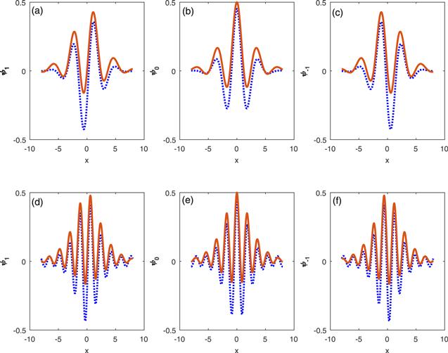
Figure 1.Stable bright solitons for c₀=−1, c₂=0.1. (a)–(c): α=1. (d)–(f): α=2. The dotted lines are numerical results by solving the GPEs with imaginary time evolution with a Gaussian initial wave package. The real curves are from the analytical solution (5).


For a more detailed analysis of these bright solitons, we attempt to find an analytical wavefunctions using the gauge method. It is of great interest that exact analytical solution can be acquired for 1D spin-1 BEC with SU(2) SOC. One challenge is the complexity of the nonlinear couplings, which is associated with c₀ and c₂ term, while the other is the spin–orbit coupling. The nonlinear couplings can be decoupled by making use of unique properties of hyperbolic functions. For a conventional spin-1 BEC, the usual bright solitonic solution for the attractive interaction is $(\tilde{{\psi }_{1}},\tilde{{\psi }_{0}},\tilde{{\psi }_{-1}})\,=A(0,{\rm{{\rm{sech}} }}({kx}),0)$. We make a gauge transformation $\psi ={e}^{i\alpha {\lambda }_{y}x}\tilde{\psi }$. Hence we obtain an analytical solution as,(5)$\begin{eqnarray}\left(\begin{array}{c}{\psi }_{1}\\ {\psi }_{0}\\ {\psi }_{-1}\end{array}\right)=A\left(\begin{array}{c}\tfrac{1}{3}-\tfrac{1}{3}\cos (\sqrt{3}\alpha x)+\tfrac{1}{\sqrt{3}}\sin (\sqrt{3}\alpha x)\\ \tfrac{2}{3}\cos (\sqrt{3}\alpha x)+\tfrac{1}{3}\\ \tfrac{1}{3}-\tfrac{1}{3}\cos (\sqrt{3}\alpha x)-\tfrac{1}{\sqrt{3}}\sin (\sqrt{3}\alpha x)\end{array}\right){\rm{sech}} ({kx}),\end{eqnarray}$where A and k are real constants with the relation $-{k}^{2}={c}_{0}{A}^{2}$.

For the bright soliton with SU(2) SOC, the $\Psi$₁ and $\Psi$₋₁ exhibits the $\sin (\alpha x)$ oscillating modulation, and $\Psi$₀ shows the $\cos (\alpha x)$ oscillating modulation. For the case with SU(3) SOC, the bright soliton in $\Psi$₁ and $\Psi$₋₁ shows a more complex oscillating modulation with a different magnitude superposition of sin and cos function under the influence of SU(3) SOC.

Figure 1 illustrates the numerical soliton sulutions and the analytical solutions with SU(3) SO coulpled BEC have the same characteristic of the symmetry and the shape. The analytic solution gives a qualitative analysis of the properties of solitons $\Psi$₁(x)=$\Psi$₋₁(−x), which replace $\Psi$₁(x)=−$\Psi$₋₁(x) in SU(2) SOC leading to mixing manifolds of ferromagnetic and antiferromagnetic states. We also note that the numerical soliton sulutions and the analytical solutions do not coincide quite as well as SU(2) SOC, but the nodes are coincident. The main reason is that the gauge transformation exhibits some spatial modulation that cannot be eliminated through local spin rotation (different from SU(2) SOC model). The analytical solutions correspond to an approximate Hamiltonian, but it shows most of the properties of the composite soliton.

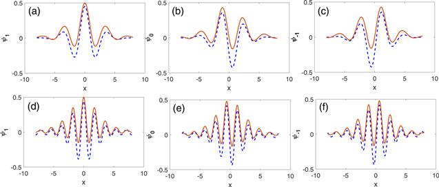
We also study the metastable states in the SU(3) SOC system. If we start from some specific initial states, the imaginary time evolution may lead to some structure as metastable solutions to the energy functional. The states have higher energy than the ground state with the same parameters. For instance, if we take a vortex-free Gaussian wave packet with a spinor (1,0,0)^T as the initial state, the numerical results get the metastable state shown in figure 2. The initial state is the ferromagnetic state, and the final state is also mixing states, which is a composite soliton. It has a similar properties as the ground state we studied.

Figure 2.

New window|Download| PPT slide
Figure 2.Metstable bright solitons for c₀=−1, c₂=0.1. (a)–(c): α=1. (d)–(f): α=2. The dotted lines are numerical results by solving the GPEs with imaginary time evolution with a Gaussian initial wave package. The real curves are from analytical solution.


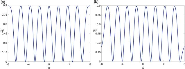
In order to study the mixing degree of the manifolds of ferromagnetic and antiferromagnetic, we calculated the value of $| F| $ in detail. For a pure antiferromagnetic state, the $| F| =0$ as in SU(2) SOC. For our composite solitons, the value of $| F| $ gradually becomes an oscillation. The value of $| F| $ gradually becomes smaller as one moves from the x space, it then becomes larger and then smaller, or vice versa. The F texture is shown in figure 3, which show a visual representation of the mixing states. When the magnetization is relatively strong, there is less antiferromagnetic ingredient. The F reflects ferromagnetic characteristics of the composite solitons.

Figure 3.

New window|Download| PPT slide
Figure 3.The magnitude of $| {\boldsymbol{F}}{| }^{2}$ along the x axis for our numerical result of metastable (a) and stable (b) for c₀=−1, c₂=0.1 and α=1.


In the last, we also performed real-time simulation of the two types of solitons as the initial state over a long time. The real-time evolution shows that the particle number in each hyperfine state is unchanged with dynamical stability.

4. Summary

We have studied the composite solitons in antiferromagnetic spin-1 Bose–Einstein condensates with SU (3) spin–orbit coupling. Different from the conventional SU(2) spin–orbit coupling, the novel gauge field has its own unique regulation mechanism. The composite solitons have novel symmetry and form stable states of mixing manifold. It shows a $| F| $ oscillation to reveal the degree of mixing manifold. Our results pave the way for exploring and engineering exotic solitons in the quantum system.

Acknowledgments

We acknowledge support from the NSF of China under grant no. 11604193, and the supported by Innovation project for graduate students in Shanxi Province (grant no. 2019SY305).

Reference View Option By original order
By published year
By cited within times
By Impact factor

[1]Perich W Anderson M H Ensher J R Cornell E A 1995 Phys. Rev. Lett. 74 3352
DOI:10.1103/PhysRevLett.74.3352 [Cited within: 1]

[2]Pethick C J Smith H 2008 Bose–Einstein Condensation in Dilute Gases Cambridge Cambridge University Press
[Cited within: 1]

[3]Morsch O Oberthaler M 2006 Rev. Mod. Phys. 78 179
DOI:10.1103/RevModPhys.78.179

[4]Combescot M Combescot R Dubin F 2017 Rep. Prog. Phys. 80 066501
DOI:10.1088/1361-6633/aa50e3

[5]Kawaguchi Y Ueda M 2012 Phys. Rep. 520 253
DOI:10.1016/j.physrep.2012.07.005 [Cited within: 5]

[6]Li L Li Z D Malomed B A Mihalache D Liu W M 2005 Phys. Rev. A 72 033611
DOI:10.1103/PhysRevA.72.033611 [Cited within: 1]

[7]Ji A C Liu W M Song J L Zhou F 2008 Phys. Rev. Lett. 101 010402
DOI:10.1103/PhysRevLett.101.010402 [Cited within: 1]

[8]Ho T L 1998 Phys. Rev. Lett. 81 742
DOI:10.1103/PhysRevLett.81.742 [Cited within: 1]

[9]Han D S Ray M W Tiurev K Ruokokoski E Gheorghe A H Möttönen M 2016 Nat. Phys. 12 478
DOI:10.1038/nphys3624

[10]Wang D S Hu X H Hu J P Liu W M 2010 Phys. Rev. A 81 025604
DOI:10.1103/PhysRevA.81.025604 [Cited within: 1]

[11]Liang Z X Zhang Z D Liu W M 2005 Phys. Rev. Lett. 94 050402
DOI:10.1103/PhysRevLett.94.050402 [Cited within: 1]

[12]Lin Y-J Jiménez-García K Spielman I B 2011 Nature 471 83
DOI:10.1038/nature09887 [Cited within: 1]

[13]Campbell D L Price R M Putra A Valdés-Curiel A Trypogeorgos D Spielman I B 2016 Nature Commun. 7 10897
DOI:10.1038/ncomms10897 [Cited within: 1]

[14]Liu Y-K Yang S-J 2014 Europhys. Lett. 108 30004
DOI:10.1209/0295-5075/108/30004 [Cited within: 2]

[15]Gautam S Adhikari S K 2014 Phys. Rev. A 90 043619
DOI:10.1103/PhysRevA.90.043619

[16]Wan N-S Yu Z-F Gao G-M Zhang A-X Xu H-P Xue J-K 2018 Mod. Phys. Lett. B. 33 1850404
DOI:10.1142/S0217984918504043 [Cited within: 1]

[17]Xu Y Zhang Y Wu B 2013 Phys. Rev. A 87 013614
DOI:10.1103/PhysRevA.87.013614 [Cited within: 1]

[18]Li Y Xue J-K 2018 Front. Phys. 13 130307
DOI:10.1007/s11467-017-0732-4 [Cited within: 1]

[19]Wan N-S Li Y Xue J-K 2019 Phys. Rev. E 99 062220
DOI:10.1103/PhysRevE.99.062220 [Cited within: 1]

[20]Kawakami T Mizushima T Nitta M Machida K 2012 Phys. Rev. Lett. 109 015301
DOI:10.1103/PhysRevLett.109.015301 [Cited within: 1]

[21]Liu Y-K Liu Y Yang S-J 2019 Phys. Rev. A. 99 063626
DOI:10.1103/PhysRevA.99.063626 [Cited within: 1]

[22]Luo X Sun K Zhang C 2017 Phys. Rev. Lett. 119 193001
DOI:10.1103/PhysRevLett.119.193001 [Cited within: 1]

[23]Han W Zhang X-F Song S-W Saito H Zhang W Liu W-M Zhang S-G 2016 Phys. Rev. A. 94 033629
DOI:10.1103/PhysRevA.94.033629 [Cited within: 4]

[24]Wang C Gao C Jian C-M Zhai H 2010 Phys. Rev. Lett 105 160403
DOI:10.1103/PhysRevLett.105.160403 [Cited within: 1]

[25]Liu Y-K Zhang C Yang S-J 2013 Mod. Phys. Lett. B. 27 1350183
DOI:10.1142/S0217984913501832 [Cited within: 1]

[26]Bao W Jaksch D Markowich P A 2003 J. Comput. Phys. 187 318
DOI:10.1016/S0021-9991(03)00102-5 [Cited within: 1]

[27]Bao W Wang H 2006 J. Comput. Phys. 217 612
DOI:10.1016/j.jcp.2006.01.020 [Cited within: 1]