1.Key Laboratory for Quantum Optics and Center of Cold Atom Physics, Shanghai Institute of Optics and Fine Mechanics, Chinese Academy of Science, Shanghai 201800, China 2.Center of Materials Science and Optoelectronics Engineering, University of Chinese Academy of Sciences, Beijing 100049, China
Fund Project:Project supported by the National Natural Science Foundation of China (Grant No. 11704391).
Received Date:22 February 2019
Accepted Date:30 April 2019
Available Online:01 July 2019
Published Online:05 July 2019
Abstract:Magnetic shielding plays an important role in magnetically susceptible devices such as cold atom clocks, atomic interferometers and other precision equipment. The residual magnetic field in a magnetic shield under a varying external magnetic field can be calculated by the Jiles-Atherton (J-A) hysteresis model and magnetic shielding coefficient. According to the calculation results, the variation of internal magnetic field can be compensated for the active compensation coils. However, it is difficult to practically obtain the exact values of the five magnetic-shielding-related parameters in the J-A hysteresis model and the other two magnetic-field-attenuation-related parameters. It usually takes a lot of time to match the parameters manually according to the measured hysteresis loop and it is difficult to ensure that the final parameters are the global optimal values. The machine learning method based on artificial neural network has been used as an efficient method to optimize the parameters of complex systems. Owing to the powerful computing capability of modern computers, using the artificial neural network to optimize parameters is usually much faster than manual optimization method, and has a greater probability of finding the global optimal parameters. In this paper, the five J-A parameters and the other two parameters relating to magnetic field attenuation are optimized by the method of online learning based on artificial neural network, and the residual magnetic field in the magnetic shield is predicted under the simulated satellite magnetic field environment. By comparing the measured residual magnetic field with the predicted value, it is found that the machine learning method can optimize the magnetic shielding characteristic parameters more quickly and accurately than the manual optimization method. This result can not only help us to compensate for the magnetic field better and optimize the parameters of our cold atom system, but also validate the application of neural network in a multi-parameter physical system. This proves that the in-depth learning neural network can be conveniently applied to other physical experiments with multi-parameter interaction, and can quickly determine the optimal parameters needed in the experiment. This application is especially effective for remote experiments with slow response to parameter adjustment, such as scientific experiments carried out on satellites or deep space. Keywords:artificial neural networks/ magnetic shielding/ hysteresis/ cold atom clock
3.实验测试装置为了模拟近地轨道的磁场环境, 我们搭建了一个准亥姆霍兹线圈, 通过控制线圈电流来控制中心轴向磁场. 该装置由三组八边形线圈构成(便于使用铝型材搭建), 线圈直径约为1.3 m, 整体高度约为1.5 m. 我们将待测屏蔽筒置于线圈内部处, 屏蔽筒直径为30 cm, 高度为80 cm, 并在屏蔽筒内部中心位置放置一个磁通门用于采集屏蔽内磁场, 在线圈轴线远离屏蔽筒处放置另一个磁通门用于采集环境磁场. 图1(a)是整个测试系统的示意图, F1和F2分别为探测环境磁场和屏蔽内部磁场的磁通门. 图1(b)是用于模拟近地轨道磁场的环境磁场变化图. 实验过程中, 首先让线圈电流产生正弦变化的环境磁场, 根据得到的磁滞回线作为神经网络训练与反馈的值来获得屏蔽筒J-A参数, 并将这组参数用于预测近地轨道环境磁场条件下的屏蔽内磁场, 将预测值和实测结果进行对比, 验证神经网络算法预测J-A参数的准确性. 图 1 (a)实验装置示意图, 同时也是有限元仿真时所用的模型图; (b)对模型进行测试所用的近地轨道环境磁场 Figure1. (a) The schematic diagram of the experimental device and also the model diagram used in our finite element simulation; (b) low Earth orbit environmental magnetic field used to test the model.
在利用神经网络对J-A参数优化之前, 除了预先设定参数范围外, 预测屏蔽内磁场还需要知道屏蔽筒内各处衰减系数SE和磁化强度与磁场之间的比例系数C, 我们使用有限元分析方法(finite element method, FEM)[31]仿真屏蔽筒内空间各处的衰减系数SE和比例系数C优化前的初始值. 图2展示了屏蔽内部一个纵向截面上有限元计算所得的SE和C. 我们探测所用磁通门置于屏蔽最中心处, 在此处的衰减系数约为31, 比例系数约为–1.8. 使用其他方法获得J-A参数时, 这两项参数一般都仅仅使用仿真值, 虽然有限元模型可能存在的各种误差, 但是往往因多参数之间关系复杂不对这两个参数进行调节. 而使用神经网络自动调节参数时, 由于神经网络具有强大的仿真计算能力, 我们将这两个参数也作为代求参数. 对SE进行有限元仿真时, 选择了厂家给出的相对磁导率, 实际上磁导率可能无法严格等于厂家给出的参数, 并且屏蔽效果可能由于形变等原因与仿真结果有一定偏差, 因此我们根据仿真结果31, 将范围限定于20—40. 对C进行有限元仿真时, 我们将磁屏蔽看作永磁体, 设置磁化强度, 能够得到空间中不同位置的感应磁场, 从而计算比例系数. 同样, 由于形变、位置偏差等一些原因, 实际结果可能也会和仿真结果有偏差, 因此根据有限元仿真结果–1.8, 因此我们将范围限定于–1.5—–2.5. 图 2 (a)数据所在磁屏蔽筒截面示意图; (b)有限元仿真所得到屏蔽内一个截面上的屏蔽效率分布图; (c)有限元仿真得到的屏蔽内一个截面上的磁化强度比例系数图 Figure2. (a) A schematic view of the section of the data; (b) the shielding efficiency distribution on a section inside the shield calculated by FEM software; (c) the magnetization intensity ratio coefficient on a section of the shield calculated by FEM software.
4.神经网络模型的建立本文需要优化的是J-A模型中的5个参数Ms, k, a, α, c和衰减系数SE以及比例系数C共7个参数. 我们建立如图3的参数优化神经网络. 图 3 神经网络调参原理示意图 使用2个隐藏层的全连接神经网络, 每层32个神经元, 一旦神经网络训练完成, 就能调用scipy库预测最优参数 Figure3. Principle of optimizing with neural network. We use 2 hidden layers of full connected neural network, 32 neurons per layer. Once the neural network training is completed, we can use scipy to predict the optimal parameters
在图3中, 神经网络作为一个复杂的函数, 我们给定输入参数值, 图中$ {x_1},{x_2}, \cdots ,{x_7}$对应J-A模型中的5个参数Ms, k, a, α, c和衰减系数SE以及比例系数C, 每一组参数可通过神经网络对应一个输出值y, 同样的参数值, 在给定环境磁场的情况下, 代入(4)和(5)式, 可以算出相应的剩余磁场, 并和实测的剩余磁场相减后求标准差y0, 我们使用神经网络这样一个通用的函数形式来拟合这个参数值到标准差的复杂过程, 一旦完成拟合, 使用scipy库[32]可以方便求出令输出值即标准差最小的参数值. 此外我们使用了在线学习的方法, 视情况将预测的参数值重新代到神经网络中进行训练, 这样可以充分利用每组参数, 用尽可能少的轮次拟合出最准确的神经网络. 神经网络模型建立过程中, 网络层数与每层的神经元数是首先需要考虑的问题[15].神经网络层数以及神经元数量会影响神经网络的性能, 如果层数较少, 或者神经元数量较少, 可能会导致无法拟合出复杂的对应关系(欠拟合), 如果层数较多, 或者神经元数量较多, 有可能会将原本简单的关系拟合复杂(过拟合). 神经元数量依惯例通常选用2的次方个, 我们尝试过64个神经元, 以及3层或4层网络, 结果显示出明显的过拟合, 即预测最优参数的标准差起伏很大且不理想, 如图4(b)所示. 我们同时也尝试过16个神经元, 2层网络, 结果显示出明显的欠拟合(所需轮次较多, 且调参结果没有32个神经元结果好). 综合上述实验, 我们认为选用2层, 每层32个神经元, 对于我们这个只有7个馈入节点的神经网络来说是比较合适的, 如图4(a)所示. 随着参数的增加, 我们需要增加神经元以及神经网络层数, 具体所需数量还要根据实验来确定. 图 4 (a)当选用2层网络各32个神经元时, 预测标准差收敛性好且最小值仅为4.9; (b)当选用3层网络各64个神经元时, 由于过拟合预测标准差振荡且最小值为27 Figure4. (a) When 32 neurons of the 2 layers network are selected, the convergence of the prediction standard deviation is good and the minimum value is only 4.9; (b) when 64 neurons of the 3 layers network are selected, the convergence of the prediction standard deviation is poor because of over-fit and the minimum value is 27.
5.参数优化结果与验证使用神经网络调参的结果如图6所示, 首先用一个正弦变化的环境磁场进行调参. 图6(a)横坐标为总循环次数, 纵坐标为我们设定的标准差, 蓝色点为初始随机地用于训练神经元的12组参数, 可见在第20轮左右, 即初始训练后预测的第8组参数就已经开始明显收敛于最优值, 最终得到的J-A参数为Ms = 540074, c = 0.58, a = 19817, k = 9.50, SE = 36.37, C = -2.37. 标准差值为4.90, 在该组参数下计算得到的磁滞回线和实测值如图6(b)所示, 红线为预测值黑线为实测值. 图 6 (a)一个典型的求参过程图, 预测参数值的标准差随实验轮次逐渐降低; (b)相应参数计算得到的磁滞回线与实测回线的比较 Figure6. (a) A typical continuation process graph, the standard deviation of the predicted parameter values is gradually reduced with the experimental round; (b) comparison of hysteresis loop and measured loop calculated by corresponding parameters.
表1手动调参和自动调参得到的参数值 Table1.Parameter values obtained by manual tuning and automatic tuning.
另外, 初始随机参数的不同可能导致不同的预测速度, 但通常都能够收敛到理想的参数点. 图7展示了另两组初始随机参数进行预测的标准差和循环轮次图, 同样蓝色点为初始随机的用于训练神经元的12组参数, 可以看出由于初始随机值不同, 在本次训练中更快达到了标准差小于5的期望值. 图 7 另外两组不同随机初始训练参数下, 标准差随实验轮次的收敛图 Figure7. Convergence graph of standard deviation with experimental rounds under two different random initial training parameters.
接着将该组参数应用于接近实际卫星在轨经历的环境磁场, 得到的结果如图8所示. 图8(a)和图8(b)分别是在环境磁场随时间变化情况下, 利用使用神经网络调参后得到的参数来计算屏蔽内磁场和实测屏蔽内磁场的对比图, 横坐标分别为时间和环境磁场; 图8(c)表示计算值和实测值的差值随时间变化曲线; 图8(d)表示计算值和实测值的差值随环境磁场变化曲线. 图中标准差越小说明计算越准确. 其中黑线是仅考虑衰减项$ {B_{SE}}$不考虑磁化项$ {B_{\rm M}}$的计算结果差值, 另外两组则分别用手动得到的参数和神经网络得到的参数来计算, 其中手动找到的参数标准差为9.33, 神经网络调参标准差为7.01. 可见使用J-A模型计算屏蔽内参数是非常必要的, 仅考虑衰减项而忽略磁滞项将会导致很大误差, 另外利用神经网络获取J-A模型的参数比手动参数更加快速准确, 为我们对空间钟磁屏蔽补偿参数的选择提供了有效的帮助. 图 8 在近地轨道磁场环境下实测磁场与计算磁场的对比图 (a)横坐标为时间; (b)横坐标为环境磁场; (c) 使用手动调节参数, 自动求得的参数, 以及仅考虑衰减项不考虑磁化项, 计算磁场与实测磁场的差值, 横坐标为时间; (d)横坐标为环境磁场 Figure8. A comparison of the measured magnetic field with the calculated magnetic field in a near-Earth orbit magnetic field environment; (a) The x axis is time; (b) the x-axis is the ambient magnetic field; (c) use manual adjustment parameters, automatically obtained parameters, and simple $ {B_{SE}}$ to calculate the difference between the magnetic field and the measured magnetic field, the abscissa is time; (d) the x-axis is the ambient magnetic field.


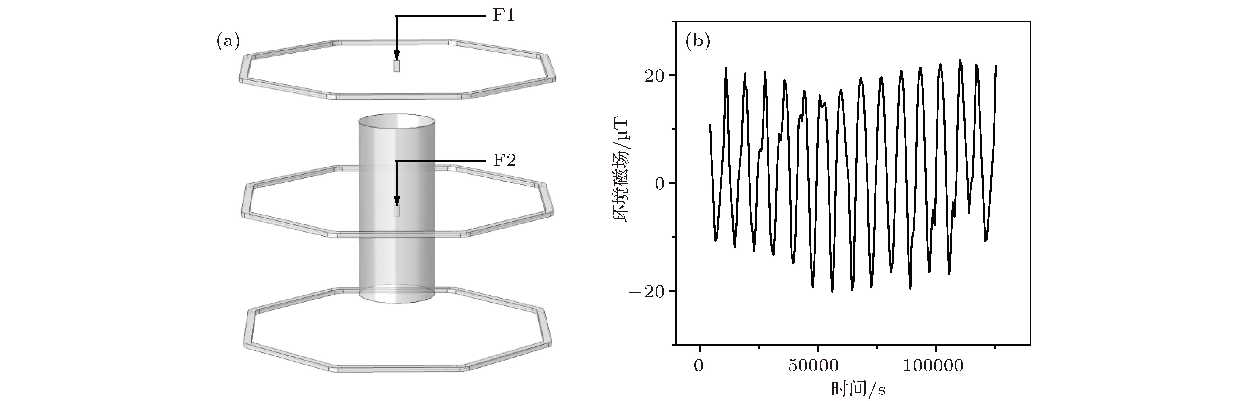 图 1 (a)实验装置示意图, 同时也是有限元仿真时所用的模型图; (b)对模型进行测试所用的近地轨道环境磁场
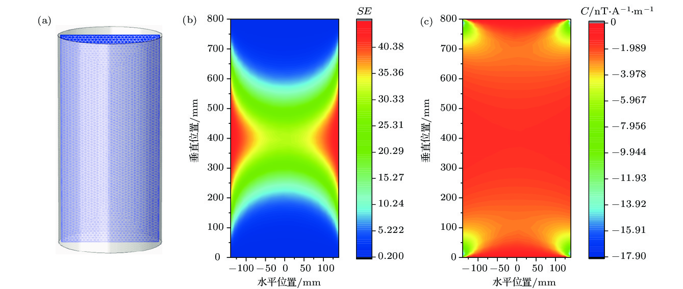 图 2 (a)数据所在磁屏蔽筒截面示意图; (b)有限元仿真所得到屏蔽内一个截面上的屏蔽效率分布图; (c)有限元仿真得到的屏蔽内一个截面上的磁化强度比例系数图
 图 3 神经网络调参原理示意图 使用2个隐藏层的全连接神经网络, 每层32个神经元, 一旦神经网络训练完成, 就能调用scipy库预测最优参数
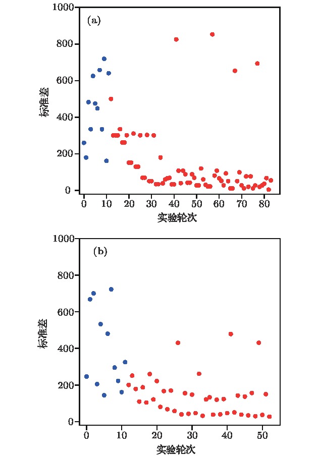 图 4 (a)当选用2层网络各32个神经元时, 预测标准差收敛性好且最小值仅为4.9; (b)当选用3层网络各64个神经元时, 由于过拟合预测标准差振荡且最小值为27
 图 5 自动调参的流程图
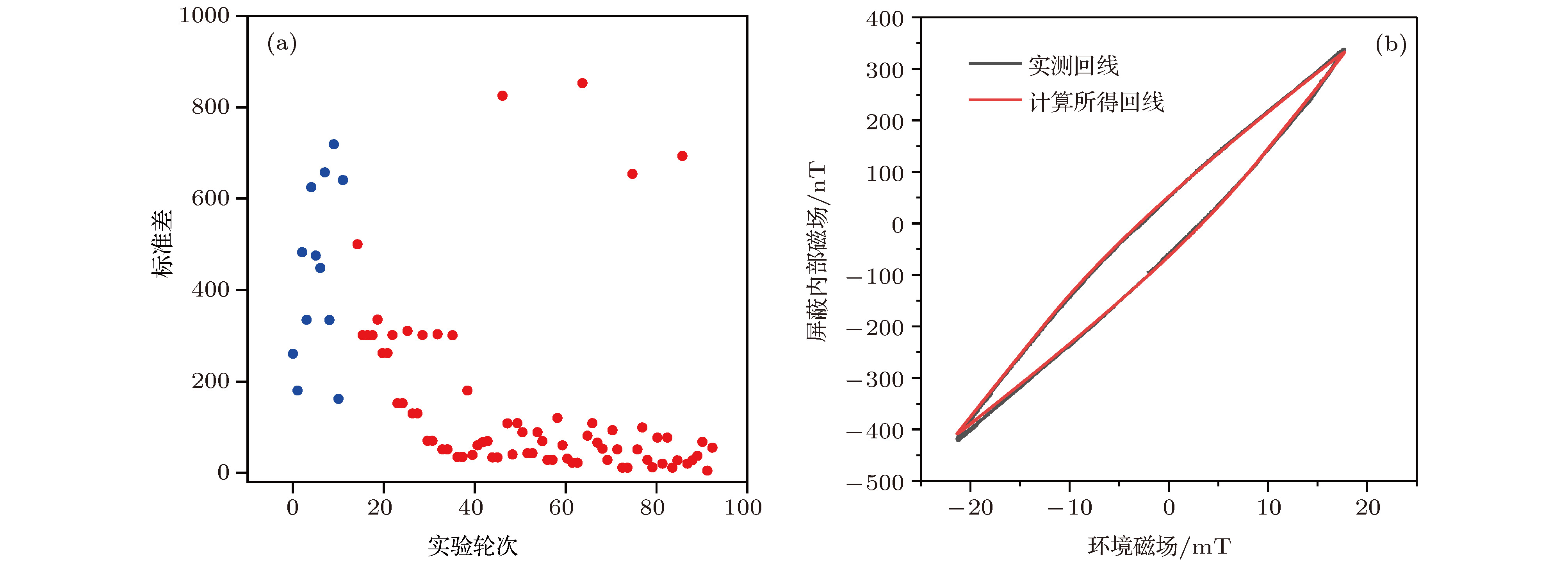 图 6 (a)一个典型的求参过程图, 预测参数值的标准差随实验轮次逐渐降低; (b)相应参数计算得到的磁滞回线与实测回线的比较
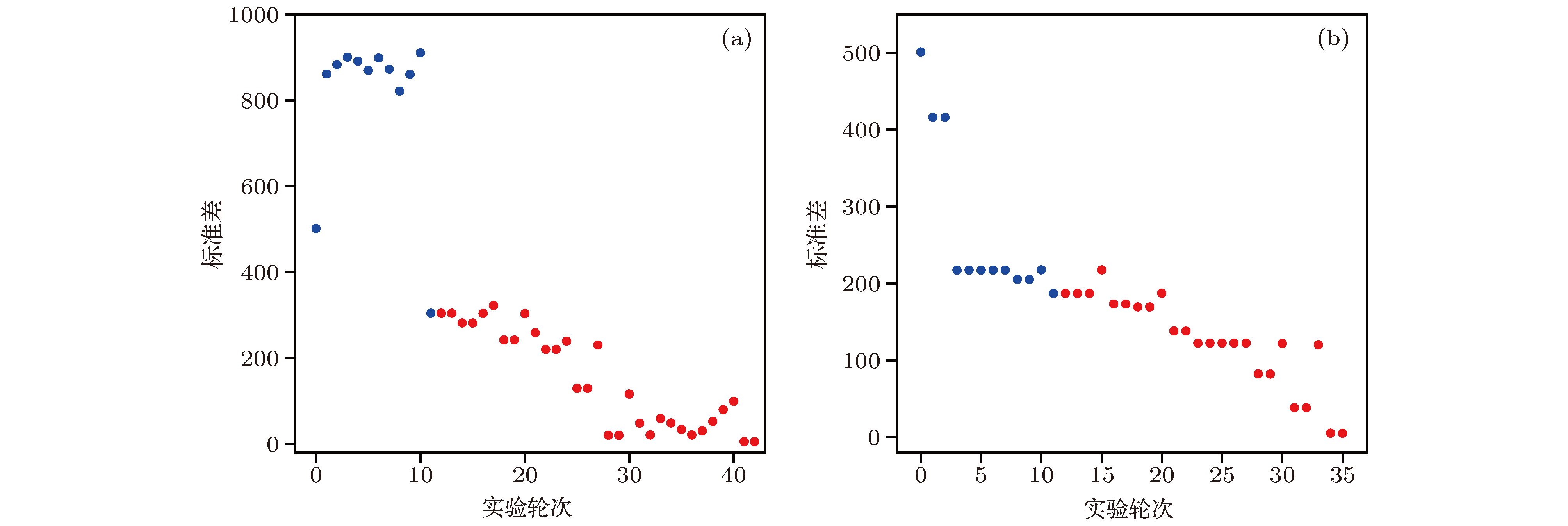 图 7 另外两组不同随机初始训练参数下, 标准差随实验轮次的收敛图

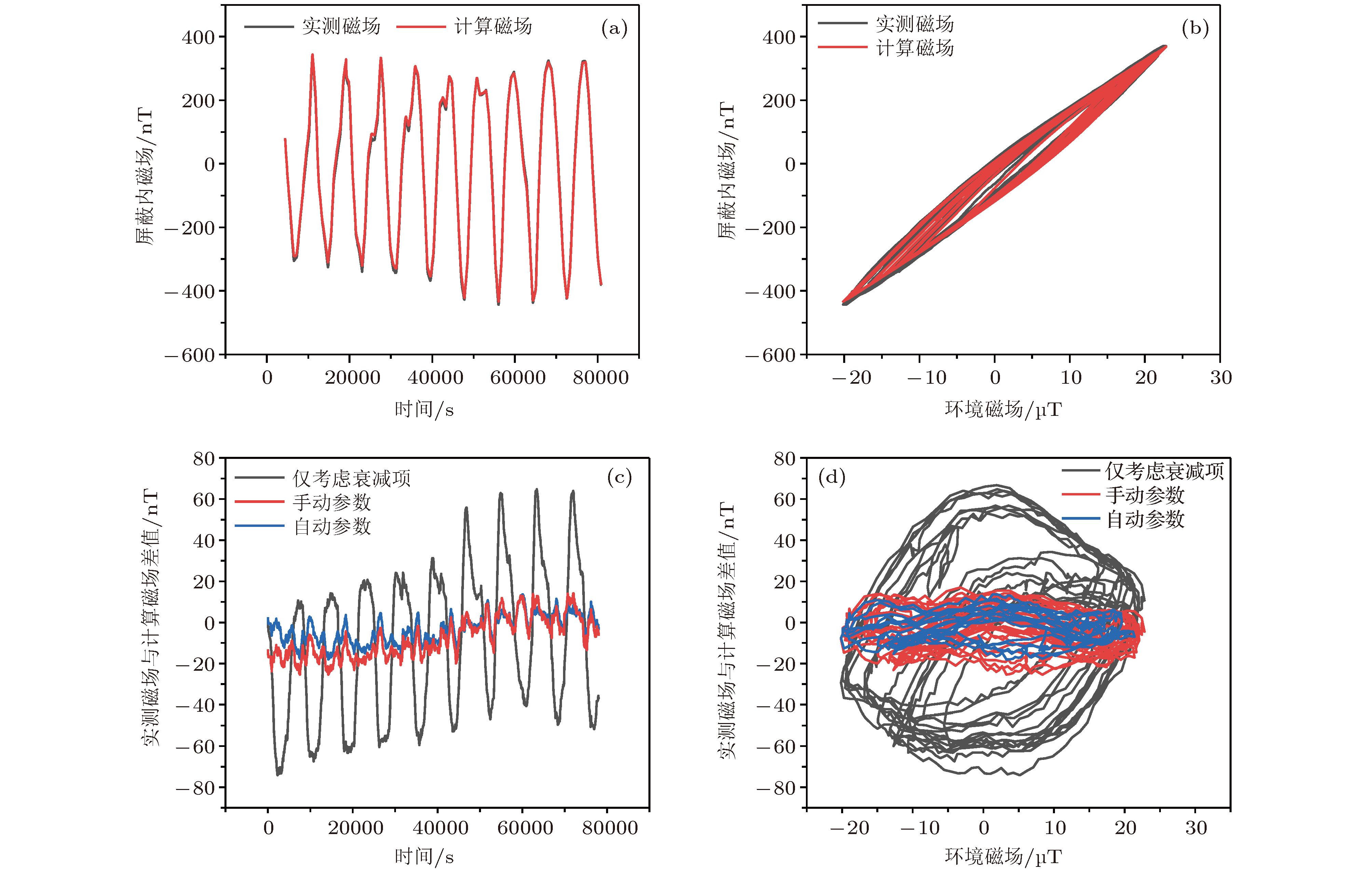 图 8 在近地轨道磁场环境下实测磁场与计算磁场的对比图 (a)横坐标为时间; (b)横坐标为环境磁场; (c) 使用手动调节参数, 自动求得的参数, 以及仅考虑衰减项不考虑磁化项, 计算磁场与实测磁场的差值, 横坐标为时间; (d)横坐标为环境磁场
