 ,2), 田强,3)北京理工大学宇航学院, 北京 100081
DYNAMICS ANALYSIS OF STOCHASTIC SPATIAL FLEXIBLE MULTIBODY SYSTEM 1)
Guo Xiang, Jin Yanfei,2), Tian Qiang,3)School of Aerospace Engineering, Beijing Institute of Technology, Beijing 100081, China通讯作者: 2) 靳艳飞, 副教授, 主要研究方向: 随机动力学; 非线性动力学与控制. E-mail:jinyf@bit.edu.cn;3) 田强, 教授, 主要研究方向: 多体系统动力学建模与分析、动力学数值计算方法. E-mail:tianq@bit.edu.cn
收稿日期:2020-08-6接受日期:2020-09-16网络出版日期:2020-11-18
| 基金资助: |
Received:2020-08-6Accepted:2020-09-16Online:2020-11-18
作者简介 About authors

摘要
轻质、高精度的柔性多体系统被广泛应用于实际工程领域中.由于实际设计公差、制造误差及环境温度等多种不确定因素的存在,使得柔性多体系统的结构参数(物理参数和几何参数)表现出随机性.具有随机结构参数的动力学模型能够客观地反映出真实系统的动力学行为,且结构参数的不确定性对空间柔性多体系统动力学响应的影响是不容忽视的.针对具有多个随机参数的空间柔性多体系统,提出了一种基于广义alpha算法的非侵入式随机柔性多体系统动力学计算方法.采用绝对节点坐标公式(absolute node coordinate formulation, ANCF)来描述柔性体, 推导建立多体系统动力学模型.利用混沌多项式展开(polynomial chaos expansion, PCE)法构建系统随机动力学方程的代理模型,然后将随机响应面法(stochastic response surface method, SRSM)嵌入广义-alpha方法中,分别采用改进抽样的回归方法(regression method of improved sampling, RMIS)和单项求容积法则(Monte Carlo simulation, MCR)来确定样本点.将数值计算结果与蒙特卡洛模拟(Monte Carlo simulation, MCS)结果进行对比, 验证了所提算法的有效性.在相同的定积分精度的条件下,根据单项求容积法则确定的样本点的计算结果稳定性更强, 且其计算效率更高.
关键词:
Abstract
Flexible multibody systems with light weight and high precision are widely used in practical engineering. The structural parameters (physical parameters and geometric parameters) of the flexible multibody system show randomness due to the existence of many uncertain factors such as actual design tolerance, manufacturing error and environmental temperature. The dynamic model with random structural parameters can objectively reflect the dynamic behavior of the real system, and the influence of the uncertainty of structural parameters on the dynamic response of the spatial flexible multibody system cannot be ignored. A non-intrusive calculation method is proposed based on the generalized-alpha algorithm to study the dynamic response of stochastic spatial flexible multibody system with multiple random parameters. The absolute node coordinate formulation (ANCF) is used to describe the flexible body, and the dynamic model of multibody system is established. The polynomial chaos expansion (PCE) method is used to construct the surrogate model of the stochastic dynamics equation of the system. Then, the stochastic response surface method (SRSM) is embedded into the generalized-alpha method. The regression method of improved sampling (RMIS) and the monomial cubature rules (MCR) are used to determine the sample points respectively. The numerical results are compared with those of Monte Carlo simulation (MCS), and the validity of the proposed algorithm is verified. Under the condition of the same definite integral precision, the calculation results of sample points determined by the monomial cubature rules are more stable and the calculation efficiency is higher.
Keywords:
PDF (697KB)元数据多维度评价相关文章导出EndNote|Ris|Bibtex收藏本文
本文引用格式
郭祥, 靳艳飞, 田强. 随机空间柔性多体系统动力学分析1). 力学学报[J], 2020, 52(6): 1730-1742 DOI:10.6052/0459-1879-20-273
Guo Xiang, Jin Yanfei, Tian Qiang.
引言
随着高新技术的发展, 在实际工程技术中,特别是轻质、高精度、柔性零部件被广泛应用于众多工程领域,如空间站柔性操作机械臂、卫星环形桁架天线、航天器太阳帆板、空间机器人等.因此, 系统各部件以刚体为假设的多刚体系统动力学不再适用当前的研究需求.传统的柔性多体系统动力学特性的描述方法存在着众多缺点,且某些动力学模型本身就不精确.在小转动和小变形假设下的公式无法精确描述多体系统柔性部件同时承受大转动和大变形的情形[1-2].Shabana[3]提出了绝对节点坐标法(absolute nodal coordinate formulation,ANCF)对具有大整体运动和大变形的柔性多体系统精确地建模.ANCF作为一种精确的非增量有限元方法,已成为柔性多体系统研究的奠基石[4-7].然而在传统的多体系统研究中, 系统的参数一般被认为是确定性的或可精确测量的.而在实际工程中,由于设计公差、装配制造误差、环境温度、摩擦、磨损等因素的存在,导致系统的材料特性、动力学参数、载荷、边界条件、初始条件等都具有不确定性,最终导致系统的刚度、质量和阻尼特性也具有不确定性. 研究表明,若将把某些不确定量 假定为某一确定性量, 是对真实模型的过度简化,甚至会得出矛盾、不合理的分析结果[8].Wu等[9]将几何参数和外力均考虑为不确定性参数,研究了不确定性参数对曲柄滑块机构的位移影响.赵宽等[10]研究了不确定性参数对旋转杆滑块系统动力学响应的影响.上述研究仅限于不确定性多刚体系统动力学,具有不确定参数的柔性多体系统的动力学研究还面临众多挑战.
工程系统建模中广泛使用的不确定性表示方法包括区间数学、模糊理论和概率分析.区间数学不需要关于参数不确定类型的信息,区间分析的目的是根据模型输入和参数的边界估计不同模型输出的边界[11-15].研究表明, 区间理论分析结果较为粗糙, 某些情况下会带来较大误差[16].模糊理论中模糊集的表示是用隶属度函数来刻画的,利用模糊算法可以计算出一个模型输出在另一个集合中的隶属度[17-19].模糊理论在描述模糊概率判断的隶属度函数时, 显得过于武断和不够精确[16].描述物理系统不确定性最广泛使用的方法就是概率分析. 基于经验积累,工程中大部分不确定性因素均可用特定的概率分布描述,且各个不确定性因素都存在其相应的物理意义.概率分析方法可以描述由随机扰动、变异性条件等引起的不确定性,且其输出的统计特性是由随机输入模型的概率分布来估计的[20].
通常不确定性分析的最终目的是统计矩和可靠性的估算. 由计算表达式不难知道,数学上的统计矩和失效概率的估算其实就是求积分. 一般情形下,对于实际工程问题的积分式都不存在封闭解,不确定性分析的本质内容就是求解其近似解.数字模拟法(抽样法)是不确定性分析中较早发展且相对简单的方法,其主要包括蒙特卡洛法[21]、重要性抽样[22]、分层抽样[23]、拉丁超立方抽样[24]和自适应抽样[25]等.局部展开法主要用来估算可靠性,主要包括一次二阶矩法[26]、一次可靠度法[27]和二次可靠度法[28]等.不确定性分析也可以通过数值积分的方式得到. 数值积分法主要用于估算统计矩,主要包括全因子数值积分法[29]、单变元降维法[30]、基于稀疏网格数值积分法[31]、随机因子法[10]等.以上几种不确定性分析方法, 功能较为单一, 只能用于估算统计矩或估算失效概率.
随机展开法是不确定性分析中一种较为经典的方法,主要包括随机配点法[32]和混沌多项式展开法 (polynomial chaos expansions,PCE) [33-34]. 其中,PCE方法最大的优势在于其能够精确地描述任意分布形式的随机变量,并能构建原随机输出变量的代理模型, 可以得到原输出量的任意不确定性信息,如统计矩、可靠性、概率密度函数等, 同样也适用于稳健性设计和可靠性设计.PCE方法大致分为侵入式混沌多项式展开(intrusive polynomial chaos expansion,IPCE)[35]和非侵入式混沌多项式展开 (non-intrusive polynomial chaosexpansion, NIPCE)[36].Sandu等[37-38]利用IPCE方法对不确定性多刚体系统响应进行分析,但是对于原模型方程较为复杂时,例如原模型的广义坐标数目或随机输入参数较多的情况,对原模型方程进行诸多改动和变换非常不便, 故此种方法不再适用;而NIPCE不需要对原模型方程进行改动, 将响应函数看作"黑箱子",仅关注输入与输出随机变量之间的函数映射关系即可.因此NIPCE被广泛用来分析不确定性动力学问题,且在实际工程问题中的应用更为广泛.
对于PCE方法, 获取PCE系数是最关键的一步, 关系着PCE模型的效率和精度.对于非侵入式混沌多项式展开法,可以采用Galerkin投影的方法[39-40]或随机响应面法 (stochastic responsesurface method, SRSM)[41]对工程系统进行不确定性分析.基于Galerkin投影的PCE方法在构建PCE模型时,构建过程以及PCE模型的形式与SRSM是完全一样的,唯一不同的地方在于估算PCE系数的方法不同.Galerkin投影的方法利用Galerkin投影来获取PCE系数, 而SRSM则是运用回归方法.
Isukapalli[41]提出的高效配点法(efficient collocation method,ECM)的优点是利用高概率区域的点较好地捕获模型的行为.由于配点的选择与多项式混沌展开的项相对应,从而避免了未知系数的线性方程组的奇异性. 但是正如Atkinson[42]所述,ECM方法不能收敛于三阶多项式混沌逼近, 这是由于配点方法的内在不稳定性造成的.特别是对于高阶多项式近似, 因为要求多项式(曲线或曲面)必须通过所有的配点,而在实际计算过程中只选择了其中部分配点, 具有一定的主观性,因此这种配点方法在本质上是不稳定的.靳红玲[43]利用改进抽样的回归方法(regression method with improvedsampling, RMIS)分析了随机平面柔性梁系统动力学响应;皮霆等[44]也利用该方法对不确定性刚柔耦合曲柄滑块机构进行了分析,该回归方法的计算成本虽高, 但其不失为一种较为稳健的估计函数逼近系数的方法.因为在该方法中使用了更多样本点的模型结果,并且每个样本点对模型的影响由所有其他样本点调节.但是由于该抽样方法得到的样本组合数呈指数增长,计算过程中不可能将所有样本点全部进行回归运算,目前仅局限于选取其中部分样本(一般取$N=2K$组, $K$为混沌多项式展开项数),存在太多主观因素, 使得计算结果的精度受到影响.单项求容积法则[45](monomial cubature rules,MCR)所产生的回归样本点组合数相对较少,且将多元积分近似为被积函数在若干离散积分节点上的函数响应值的加权和,得到具有较高代数精度的积分形式.
本工作采用ANCF来描述含多个随机参数的空间柔性多体系统,基于广义alpha算法提出了一种非侵入式的混沌多项式计算方法来求解随机微分-代数方程组.同时对比了当前几种统计矩估算方法的计算效率,得出采用MCR方法确定的样本点组数相对较少, 从而提高了计算效率.此外通过数值算例发现,随机参数对空间柔性多体系统动力学响应的影响是不可忽视的.本工作以期为分析随机柔性多体系统的动力学行为提供参考.
1 含随机参数的柔性多体系统
本文采用ANCF描述缩减三维曲梁单元的变形[46],利用相关动力学原理可得到系统动力学的微分代数方程其中, ${M}$为系统广义质量阵, ${q}$为系统广义坐标, ${Q}$为系统广义外力, ${F}$为系统广义弹性力, ${\varPhi}$和${\varPhi }_{q} $分别为系统约束方程以及对广义坐标的Jacobi矩阵, ${\lambda}$为Lagrange乘子.
系统中第$i$个单元的质量阵可表示为
利用ANCF建模得到的系统质量矩阵为常数矩阵. 由虚功原理
可得到系统广义外力为
其中, $\delta {W}_{{e}}^{i} $表示单元外力的虚功, ${f}^{i}$表示外力矢量.
文献[46]根据虚功原理并采用第一类Pioa-Kirchhoff应力张量的方法推导得到弹性力${F}$及其Jacobi矩阵的解析表达式可使基于ANCF建模的计算效率大大提高.
根据方程(1), 可将含随机参数的柔性多体系统动力学方程可表示为
其中, 带"$\sim $"的矩阵和向量均为含有随机参数的矩阵和向量,随机变量${\xi}=\left[ \xi _{1} ,\xi _{2} ,\cdots ,\xi _{d}\right],$第$i$个随机参数可表为${\xi }_{i} \left( {i=1, 2, \cdots ,d}\right)$的函数, $d$为随机参数个数.
2 非侵入式混沌多项式计算方法
针对随机微分-代数方程组(5), 本节介绍一种非侵入式混沌多项式计算方法.2.1 混沌多项式展开
设随机过程${Y}$可利用混沌多项式[16]表为式中$H_{n} \left(\xi_{i_{1}} ,\xi _{i_{2}} ,\cdots ,\xi_{i_{n}}\right)$表示$n$阶Hermite正交多项式, ${\xi }_{i_{1}} ,{\xi }_{i_{2}},\cdots,{\xi }_{i_{n} } $为标准正态随机变量.由于Hermite正交多项式对应正态随机变量,故在构建PCE模型之前需要将输入的非正态分布随机变量转化为标准正态随机变量[47].对式(6)进行简化并截断后得到
其中, $H_{i} \left( {{\xi }} \right)$为$p$阶Hermite正交多项式, ${\xi }=\left[ {\xi }_{1} ,{{\xi }_{2} ,\cdots ,{\xi }_{d} }\right],\alpha_{i} $为待定系数. ${Y}$的展开项数
其中, $d$为输入随机变量维数, $p$为混沌多项式展开的阶数. 阶数越高截断误差越小, 展开项数越多. 结合实际计算情况,一般取$p=2$或$p=3$时的PCE模型即可得到较为精确的结果.
2.2 随机系统动力响应分析
2.2.1 随机响应面法将系统的输入输出变量全部用混沌多项式展开之后,为求得系统输出响应的统计矩信息, 需要得到待定系数的信息.对于非侵入式混沌多项式的不确定性分析方法,最常用的方法就是随机响应面法[16], 图1为随机响应面法的计算流程图.随机响应面法主要包括抽样、随机响应面的构建.
图1
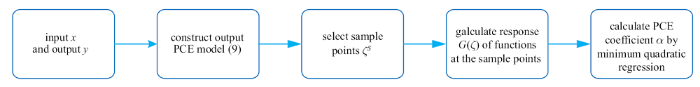 新窗口打开|下载原图ZIP|生成PPT
图1随机响应面法流程图
Fig. 1Flow chart of SRSM
Step 1 随机响应面的构建.
设${y}=f\left( {{x}} \right)$的输出响应的$p$阶混沌多项式展开为
其中, ${\xi }$为$d$维标准随机变量, 一般情况$d$与随机输入变量${x}$的维数的相同, $\alpha_{i}$是待定的PCE系数.
Step 2 估算PCE模型中的系数.
①选取有效的样本点. 设回归采样策略中所用到的样本点数目为$N$.在标准随机空间中选取$N$个有效样本${\xi }^{S}=\left[{\xi}_{1}^{S} ,{{\xi}_{2}^{S} ,\cdots ,{\xi }_{j}^{S} ,\cdots ,{\xi }_{N}^{S} }\right]^{T},$其中${\xi }_{j}^{S} =\left[ {\xi}_{j1}^{S} ,{{\xi}_{j2}^{S} ,\cdots ,{\xi }_{jd}^{S} }\right],$角标"$S$"所表示的量为样本点.
②将样本点从标准随机空间变换到原随机空间${x}^{S}=\left[{x}_{1}^{S} ,{{x}_{2}^{S} ,\cdots ,{x}_{j}^{S} ,\cdots ,{x}_{N}^{S}} \right]^{T},$其中${x}_{j}^{S} =\left[x_{j1}^{S} ,{x_{j2}^{S} ,\cdots,x_{jd}^{S} } \right]$. 原随机空间中第$j$个样本点的第$i$维样本点$x_{ji}^{S}=T_{i} \left( {\xi_{ji}^{S} } \right)$其中变换$T_{i} \left( {\xi_{ji}^{S}} \right)=\mu_{x_{i} } +\sigma_{x_{i} } \xi_{ji}^{S}$, $\mu_{x_{i} }$和$\sigma_{x_{i} } $分别对应第$i$维随机输入变量的均值和标准差.
③在样本点${x}^{S}=\left[ {{x}_{1}^{S} ,\cdots,{x}_{j}^{S} ,\cdots ,{x}_{N}^{S} }\right]^{T}$上调用原模型的输出响应, 得到各样本点响应的函数值
④利用最小二次回归估算PCE系数. 将样本点${\xi }^{S}=\left[{\xi }_{1}^{S} ,{{\xi }_{2}^{S} ,\cdots ,{\xi }_{j}^{S} ,\cdots ,{\xi}_{N}^{S} } \right]^{T}$和函数响应${G}\left( {{\xi }}\right)$分别代入式(9)得$\tilde{A} \left(\xi\right)\alpha =G( \xi),$其中
根据线性最小二次回归可得
2.2.2 单项求容积法则
关于随机响应面法 Step 2 中样本点的选取,另一种有效的方法是单项求容积法则[45].运用MCR获得回归的样本点的优势在于:可以运用较少的积分点数得到较高代数精度的积分形式,且由MCR产生的样本点可以全部用来估算PCE系数, 保证了不确定性传播的精度.适用于具有$5$阶精度$d\left( {d\geqslant 3} \right)$维变量的MCR公式为
其中
式(14)中求和号下面的"permutation"意为对括号中的数做全排列,式(14)中第一项排列结果为$\left( {r,0,\cdots ,0} \right)$, $\left({0,r,0,\cdots ,0} \right)$, $\cdots$, $\left( {0,\cdots ,0,r} \right)$, $(-r,0,\cdots ,$ $0),$ $\left( {0,-r,0,\cdots ,0} \right),\cdots,\left( {0,\cdots ,0,-r} \right),$第二项同样对$\pm s$作全排列,$A,B,C,D$为常数. 本文在求解PCE系数时只需对公式中给出的样本点进行回归计算,总的样本点组数为$N_{1} =2^{d}+2d$.虽然式(14)的样本点组数比文献[43]中的公式I增加较多,但对于较高维变量的问题具有较好的计算稳定性.
适用于具有$7$阶精度$d\left( {d=3,4,6,7} \right)$维变量的MCR公式为
其中
积分点个数为$N_{2} =2^{d}+2d^{2}+1$.
2.2.3 随机输出响应变量的数字特征
利用随机响应面法得到PCE的系数之后,可以较为方便的得出随机输出响应变量的数字特征
2.3 非侵入式随机微分代数方程组计算方法
将方程组(5)通过差分直接离散成随机代数方程组进行求解, 迭代过程如下其中
广义alpha算法的参数取值为
其中, 算法谱半径$\rho \in \left[ {0,1} \right],\rho $取值越大耗散越小, 本文取$\rho =0.8$. 设方程组(5)的解为
其中, $\tilde{q} ,\tilde{\lambda } $分别为随机广义坐标以及随机拉格朗日乘子, 定义在第$n$个时间步长上的非线性方程组为
非线性方程组(27)可由Newton-Raphson迭代求解
式中$i$表示第$i$次Newton-Raphson迭代, ${J}$为${Y}$关于${V}$的Jacobian矩阵
其中
$\hat{\beta}=\frac{1-\alpha_{m} }{h^{2}\beta \left({1-\alpha_{f} } \right)}.$
本文提出的求解随机微分代数方程组的非侵入式计算方法流程图如图2所示,首先针对系统中所含的随机参数选取$N$组样本点,样本点组数$N$由具体的采样方法、PCE阶数及随机变量维数确定; 其次,随机响应面法与广义alpha算法相结合, 将 SDAEs转化为若干组确定性非线性代数方程组.图2中样本点$\xi^{S}=\left[ \xi_{1}^{S} ,\xi_{2}^{S} ,\cdots ,\xi_{N}^{S} \right]$简写为$\xi =\left[ \xi_{1} ,\xi_{2} ,\cdots ,\xi_{N} \right],\xi_{j}^{S} $简写为$\xi_{j} ,j=1,2,\cdots N$. $\xi_{j}$为具体某一组采样的样本点, $tol$为Newton-Raphson迭代过程中的收敛误差,$T\!fin$, $h$分别为总仿真时长和时间步长. 得到PCE的系数后,根据式(21)和式(22)可计算输出响应的均值和标准差.
图2
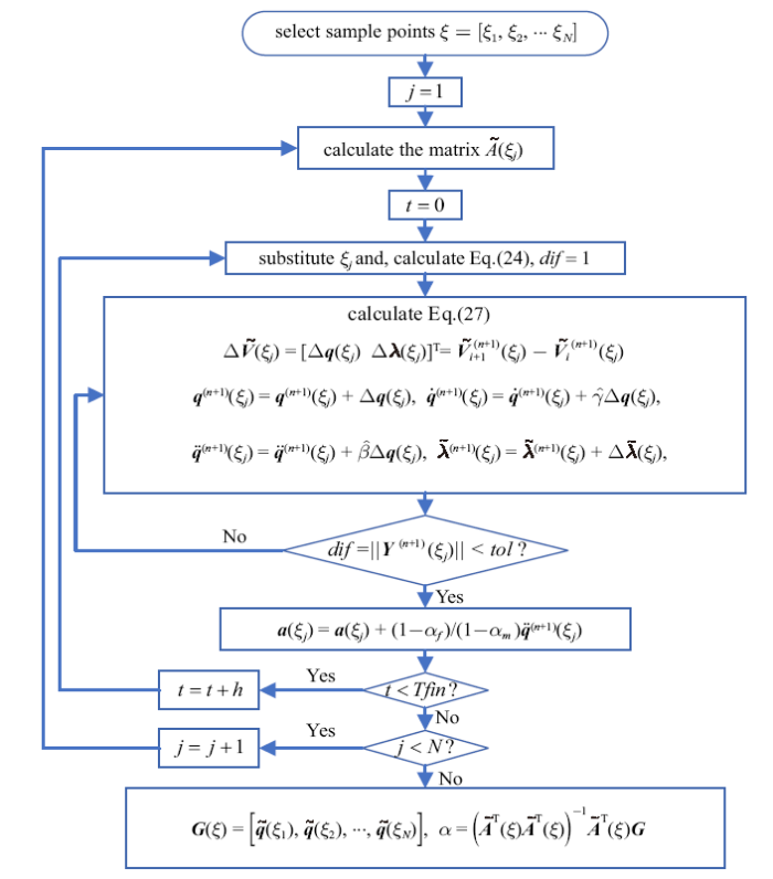 新窗口打开|下载原图ZIP|生成PPT
图2非侵入式随机微分代数方程组求解算法
Fig. 2The non-intrusive computation methodology for solving stochastic DAEs
3 数值算例
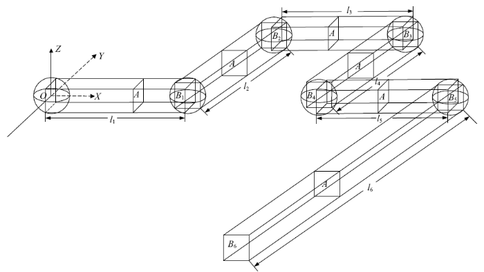
如图3所示, 空间六连杆柔性多体系统的各杆长度分别为$l_{1} =l_{2} =l_{3} =l_{4}=l_{5} =2$ m, $l_{6} =4$ m, 密度和杨氏模量分别为$\rho =2767$ kg/m$^{3}$, $E=6.895\times10^{10}$ Pa.本文对空间六连杆柔性多体系统分别使用含$4,4,4,4,4,8$个ANCF缩减梁单元对各杆进行建模.为了获得更加精确的结果, 避免所采用的ANCF单元产生泊松闭锁问题[48-49],本文不考虑梁单元的泊松效应, 假定泊松比为零.梁的截面积和惯性矩分别为$A=7.299\times 10^{-5}$ m$^{2}$, $I=8.215\times10^{-9}$ m$^{4}$. 设重力加速度$g=9.81$ m/s$^{2}$, 初始状态为水平, 考察系统在重力作用下的动态过程.现设空间六连杆柔性多体系统的密度、杨氏模量、截面积和转动惯量为服从正态分布的随机变量,即$\tilde{\rho} =\rho +r_{1} \rho \xi_{1}$, $\tilde{E}=E+r_{2} E\xi_{2}$, $\tilde{A} =A+r_{3} A\xi_{3}$, $\tilde{I} =I+r_{4} I\xi_{4}$, $r_{i}$ $\left( {i=1,2,3,4} \right)$为不确定性系数.此外, 所使用的计算机主要参数为8核主频2.3 GHz的CPU和8 GB内存, 本文算例的仿真时间步长均为$5\times 10^{-4}$ s.图3
 新窗口打开|下载原图ZIP|生成PPT
图3空间六连杆柔性多体系统示意图
Fig. 3Schematic view of the spatial flexible multibody system
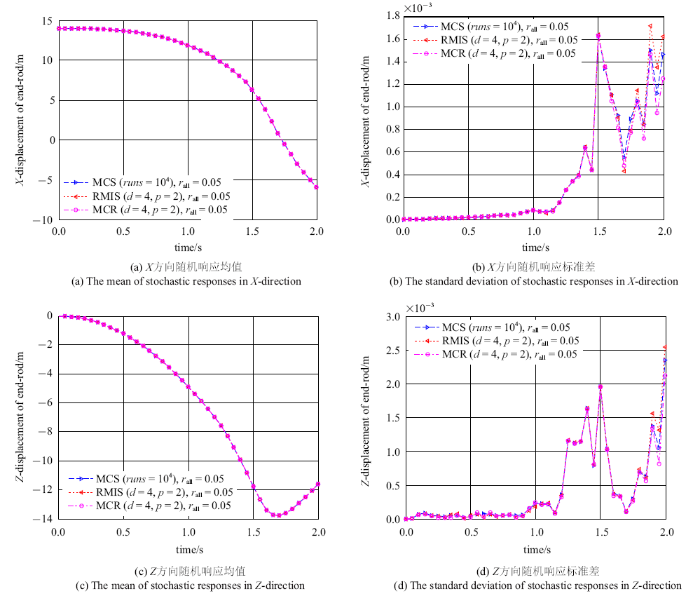
图4给出了不确定性系数$r_{i} =0.05$ $(i=1,2,3,4)$时的运动过程, 基于混沌多项式的随机响应面法, 分别采用改进抽样的回归方法(RMIS)及单项求容积法则(MCR)所选取的样本点计算随机空间六连杆柔性多体系统末端点$B_{6}$的$X$方向和$Z$方向位移响应的均值和标准差. 图4(a)和图4(c)分别给出了系统末端点$B_{6}$的$X$方向和$Z$方向位移随机响应的均值; 图4(b)和图4(d)为末端点$B_{6}$的$X$方向和$Z$方向位移随机响应的标准差, 并分别与蒙特卡洛模拟(MCS)$10^{4}$次的结果对比. 由于MCS计算成本较高, 故只对比前2 s的运动过程,三种方法MCR, RMIS, MCS的计算时间分别为629.65 s, 783.77 s, $2.519 3\times10^{5}$ s.结果显示MCR方法所得结果与MCS方法基本吻合,RMIS方法在确定样本点时具有一定的主观性, 造成其计算结果较为不稳定.
图4
 新窗口打开|下载原图ZIP|生成PPT
图4系统末端点位移响应
Fig. 4Displacement response at the end point of the system
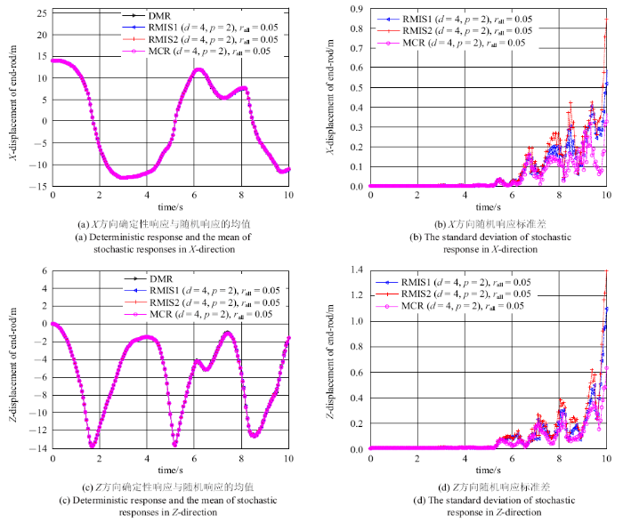
为了进一步研究空间六连杆柔性多体系统在较长时间的运动过程,图5给出了不确定性系数$r_{i} =0.05$ $\left( {i=1,2,3,4}\right)$时空间六连杆柔性多体系统的末端点的位移随时间变化的历程图,仿真时间为10 s. 其中图5(a)和图5(c)分别给出了系统末端点$B_{6}$的$X$方向和$Z$方向位移的确定性模型响应(deterministic model response, DMR)与随机响应的均值, 图5(b)和图5(d)为$X$方向和$Z$方向随机响应的标准差.随机响应的均值和标准差全都分别用RMIS和MCR方法计算得到, 且其混沌多项式展开阶数均为$p=2$, 不确定性系数$r_{all}=0.05$等价于$r_{i}=0.05$ $(i=1,2,3,4)$. 由于RMIS方法在选择样本点时, 不同的样本点组合计算得出的结果都是不相同的,RMIS1和RMIS2分别为不同的样本点组合的情况, 造成其计算结果不稳定. 而MCR方法所确定的样本点可以全部用于计算过程, 其计算结果比RMIS方法较为稳定.
图5
 新窗口打开|下载原图ZIP|生成PPT
图5含4个随机参数的系统末端点位移响应
Fig. 5Displacement response at the end point of the system with four random parameters
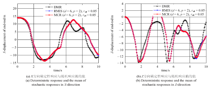
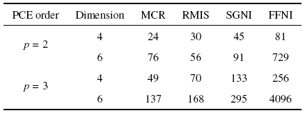
此外, RMIS方法除了计算结果具有不稳定性, 其计算效率较MCR方法也是大打折扣.假设空间六连杆柔性多体系统各杆长度为服从正态分布的随机变量, 即$l_{i} =l_{i} +r_{i} l_{i} \xi_{i}$, $i=1,2,\cdots ,6,r_{i} $为不确定性系数, 其余参数取值与上述算例一致.图6(a)和图6(b)分别给出了系统末端点$B_{6}$的$X$方向和$Z$方向位移的确定性模型响应(deterministic model response,DMR)与随机响应的均值. 其中随机响应的PCE展开阶数为$p=2,$不确定性系数$r_{all}=0.05$等价于$r_{i} =0.05$ $( i=1,2,\cdots ,6)$. 表1给出了当PCE阶数分别为$2$和$3$时, 随机变量维数分别为$4$和$6$时,MCR方法、RMIS方法、SGNI方法和FFNI方法分别所需的样本点组数. 结果显示: MCR方法的计算效率相对较高, RMIS和SGNI方法次之,FFNI所需的样本点组数随着PCE的阶数和随机变量维数的增大呈指数上升.
图6
 新窗口打开|下载原图ZIP|生成PPT
图6含6个随机参数的系统末端点位移响应
Fig. 6Displacement response at the end point of the system with six random parameters
Table 1
表1
表1四种方法所需样本点组数
Table 1
 |
新窗口打开|下载CSV
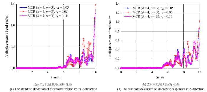
为了深入研究各个随机参数对空间六连杆柔性多体系统动力学响应的影响,图7~图10分别为$d=4$, $p=3$, $r_{all} =0.05$时,密度、杨氏模量、截面积及惯性矩的不确定性系数分别为$0.05,0.1$时系统末端点$X$方向和$Z$方向位移的标准差.当密度、截面积参数的不确定性系数取$0.05$时要比$0.1$时对随机系统$X$方向和$Z$方向位移响应的影响都较为显著;杨氏模量和惯性矩参数的不确定性系数取$0.05$时对随机系统$X$方向位移响应的影响较为显著,取$0.1$时对随机系统$Z$方向位移响应的影响较为显著.
图7
 新窗口打开|下载原图ZIP|生成PPT
图7材料密度的不确定性对系统末端点位移响应的影响
Fig. 7The influence of the uncertainty of material density on the displacement response of the end point of the system
图8
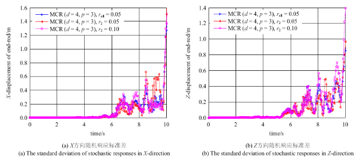 新窗口打开|下载原图ZIP|生成PPT
图8杨氏模量的不确定性对系统末端点位移响应的影响
Fig. 8The influence of the uncertainty of Young's modulus on the displacement response of the end point of the system
图9
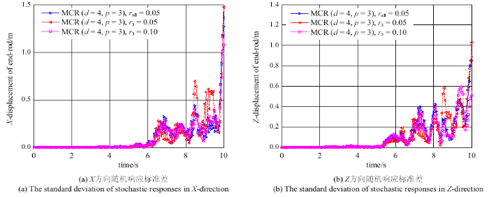 新窗口打开|下载原图ZIP|生成PPT
图9梁截面积的不确定性对系统末端点位移响应的影响
Fig. 9The influence of the uncertainty of beam cross-sectional area on the displacement response of the end point of the system
图10
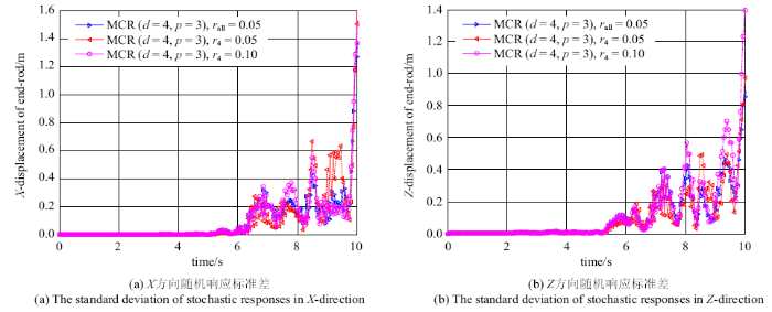 新窗口打开|下载原图ZIP|生成PPT
图10惯性矩的不确定性对系统末端点位移响应的影响
Fig. 10The influence of the uncertainty of area moment of inertia on the displacement response of the end point of the system
表2给出了随机系统前10 s内,各个参数的不确定性对随机系统响应的数字特征最大绝对值的影响(结果保留4位小数).结合表2以及图7~图10可以得出: 各个随机参数不确定性对随机系统的均值响应影响较小, 但是对随机系统的标准差影响较为显著. 其中, 杨氏模量和惯性矩的分散性对随机系统$X$方向位移响应的影响较大; 密度和截面积的分散性对随机系统$Z$方向位移响应的影响较大.
Table 2
表2
表2随机参数对随机系统响应数字特征的影响
Table 2
 |
新窗口打开|下载CSV
4 结论
本文针对具有多个随机参数的不确定性柔性多体系统,提出了一种基于广义alpha算法的非侵入式计算方法.采用ANCF的缩减梁单元对柔性体进行网格划分.首先利用广义alpha算法直接将随机微分代数方程组转化为非线性随机代数方程组.然后利用PCE方法构建系统代理模型, 在此基础上采用SRSM求解PCE的待定系数.在应用SRSM方法时分别用RMIS和MCR方法进行采样, 并用MCS验证了结果的正确性,同时通过数值仿真得到: 与RMIS方法相比, MCR方法的计算结果更加稳定;且与其他方法相比MCR方法的计算效率更高.本文采用MCR采样策略, 对含有随机参数的空间柔性多体系统的动力学行为进行研究.仿真结果表明参数的不确定性对随机系统响应的影响是不可忽视的. 数值结果表明,本文提出的计算方法对研究含有多个随机参数的柔性多体系统的动力学特性是有效和适用的.
参考文献 原文顺序
文献年度倒序
文中引用次数倒序
被引期刊影响因子
DOIURL [本文引用: 1]
DOIURL [本文引用: 1]
[本文引用: 1]
[本文引用: 1]
DOIURL
DOIURL
[本文引用: 1]
[本文引用: 1]
URL [本文引用: 1]

随机分析方法、模糊分析方法是已经广泛使用的工程结构不确定性分析方法, 近年来区间分析方法逐渐为人们所熟知并成为是一种新的工程结构不确定性分析方法,它主要用来研究具有区间特性的工程结构. 区间分析方法在统计信息不足以描述不确定参数的概率分布或隶属函数、工程单位仅提供不确定参数的区间范围而想获得结构响应的区间范围时就发挥了其优点. 综述了区间分析方法及其在工程结构不确定性分析中的应用状况, 将基于区间分析的工程结构不确定性问题研究归结为以下4个方面: 不确定性结构系统的区间有限元分析; 基于区间的非概率可靠性分析; 工程结构区间反演分析; 基于区间参数的结构优化设计. 分析评价了国内外在这几个方面的研究成果及其最新进展, 同时指出目前研究中存在的问题和研究的方向.
URL [本文引用: 1]
Stochastic analysis method and fuzzy analysis method arewidely used in uncertainty analysis of engineering structures. Recently,interval analysis method is gradually known and becomes a newuncertaintyanalysis method. Interval analysis method is mainly used for engineeringstructures with interval properties. Interval analysis method shows itsmerits when the statistical information does not available for the parameters'probability distributions or related functions except the intervals of theparameters. In this paper, interval analysis method and itsapplications in engineering structure uncertainty analysis are overviewed. Theapplications are summarized into four parts, that is, interval finiteelement analysis in uncertainty of engineering structures; the probability basedon interval analysis; interval inverse analysis method of engineeringstructures; structural optimum design based on interval parameters. Theresearch results and recent advances in these parts are analyzed,and the existing problems and future trends in these fields arediscussed.
[本文引用: 1]
[本文引用: 2]
[本文引用: 2]
DOIURL [本文引用: 1]
DOIURL
DOIURL [本文引用: 1]
[本文引用: 4]
[本文引用: 4]
DOIURL [本文引用: 1]
Uncertainty propagation in complex engineering systems with fuzzy variables constitutes a significant challenge. This paper proposes a Polynomial Chaos type spectral approach based on orthogonal function expansion. A fuzzy variable is represented as a set of interval variables via the membership function. The interval variables are further transformed into the standard interval [-1,1]. Smooth nonlinear functions of standard interval variables are projected in the basis of Legendre polynomials by exploiting its orthogonal properties over the interval [-1,1]. The coefficients associated with the basis functions are obtained by a Galerkin type of error minimisation. The method is first illustrated using scalar functions of multiple fuzzy variables. Later the method is proposed for elliptic type finite element problems where the technique is extended to vector valued functions with multiple fuzzy variables. The response of such systems can be expressed in the complete basis of multivariate Legendre polynomials. The coefficients, obtained by Galerkin type of error minimisation, can be calculated from the solution of an extended set of linear algebraic equations. An eigenfunction based model reduction technique is proposed to obtain the coefficient vectors in an efficient way. A numerical example of axial deformation of a rod with fuzzy axial stiffness is considered to illustrate the proposed methods. Linear and nonlinear membership functions are used and the results are compared with direct numerical simulation results. (C) 2013 Elsevier B.V.
DOIURL
DOIURL [本文引用: 1]
[本文引用: 1]
[本文引用: 1]
DOIURL [本文引用: 1]
[本文引用: 1]
[本文引用: 1]
DOIURL [本文引用: 1]
[本文引用: 1]
[本文引用: 1]
DOIURL [本文引用: 1]
DOIURL [本文引用: 1]
[本文引用: 1]
DOIURL [本文引用: 1]
DOIURL [本文引用: 1]
DOIURL [本文引用: 1]
[本文引用: 1]
[本文引用: 1]
[本文引用: 1]
[本文引用: 1]
DOIURL [本文引用: 1]
DOIURL [本文引用: 1]
This study explores the use of generalized polynomial chaos theory for modeling complex nonlinear multibody dynamic systems in the presence of parametric and external uncertainty. The polynomial chaos framework has been chosen because it offers an efficient computational approach for the large, nonlinear multibody models of engineering systems of interest, where the number of uncertain parameters is relatively small, while the magnitude of uncertainties can be very large (e.g., vehicle-soil interaction). The proposed methodology allows the quantification of uncertainty distributions in both time and frequency domains, and enables the simulations of multibody systems to produce results with “error bars”. The first part of this study presents the theoretical and computational aspects of the polynomial chaos methodology. Both unconstrained and constrained formulations of multibody dynamics are considered. Direct stochastic collocation is proposed as less expensive alternative to the traditional Galerkin approach. It is established that stochastic collocation is equivalent to a stochastic response surface approach. We show that multi-dimensional basis functions are constructed as tensor products of one-dimensional basis functions and discuss the treatment of polynomial and trigonometric nonlinearities. Parametric uncertainties are modeled by finite-support probability densities. Stochastic forcings are discretized using truncated Karhunen-Loeve expansions. The companion paper “Modeling Multibody Dynamic Systems With Uncertainties. Part II: Numerical Applications” illustrates the use of the proposed methodology on a selected set of test problems. The overall conclusion is that despite its limitations, polynomial chaos is a powerful approach for the simulation of multibody systems with uncertainties.]]>
DOIURL [本文引用: 1]
This study applies generalized polynomial chaos theory to model complex nonlinear multibody dynamic systems operating in the presence of parametric and external uncertainty. Theoretical and computational aspects of this methodology are discussed in the companion paper “Modeling Multibody Dynamic Systems With Uncertainties. Part I: Theoretical and Computational Aspects”.In this paper we illustrate the methodology on selected test cases. The combined effects of parametric and forcing uncertainties are studied for a quarter car model. The uncertainty distributions in the system response in both time and frequency domains are validated against Monte-Carlo simulations. Results indicate that polynomial chaos is more efficient than Monte Carlo and more accurate than statistical linearization. The results of the direct collocation approach are similar to the ones obtained with the Galerkin approach. A stochastic terrain model is constructed using a truncated Karhunen-Loeve expansion. The application of polynomial chaos to differential-algebraic systems is illustrated using the constrained pendulum problem. Limitations of the polynomial chaos approach are studied on two different test problems, one with multiple attractor points, and the second with a chaotic evolution and a nonlinear attractor set.]]>
[本文引用: 1]
[本文引用: 1]
[本文引用: 1]
[本文引用: 2]
[本文引用: 1]
[本文引用: 2]
[本文引用: 2]
[本文引用: 1]
[本文引用: 1]
[本文引用: 2]
[本文引用: 2]
[本文引用: 2]
DOIURLPMID [本文引用: 1]
This study outlines a drug delivery mechanism that utilizes two independent vehicles, allowing for delivery of chemically and physically distinct agents. The mechanism was utilized to deliver a new anti-cancer combination therapy consisting of piperlongumine (PL) and TRAIL to treat PC3 prostate cancer and HCT116 colon cancer cells. PL, a small-molecule hydrophobic drug, was encapsulated in poly (lactic-co-glycolic acid) (PLGA) nanoparticles. TRAIL was chemically conjugated to the surface of liposomes. PL was first administered to sensitize cancer cells to the effects of TRAIL. PC3 and HCT116 cells had lower survival rates in vitro after receiving the dual nanoparticle therapy compared to each agent individually. In vivo testing involved a subcutaneous mouse xenograft model using NOD-SCID gamma mice and HCT116 cells. Two treatment cycles were administered over 48 hours. Higher apoptotic rates were observed for HCT116 tumor cells that received the dual nanoparticle therapy compared to individual stages of the nanoparticle therapy alone.
DOIURL [本文引用: 1]
DOIURL [本文引用: 1]
