 , 徐兵兵, 吕军, 彭海峰
FREE ELEMENT METHOD AND ITS APPLICATION IN STRUCTURAL ANALYSIS1)
GaoXiaowei, XuBingbing, LüJun, PengHaifeng中图分类号:O341
文献标识码:A
通讯作者:
收稿日期:2019-01-7
网络出版日期:2019-05-18
版权声明:2019力学学报期刊社 所有
基金资助:
展开
摘要
关键词:
Abstract
Keywords:
-->0
PDF (9187KB)元数据多维度评价相关文章收藏文章
本文引用格式导出EndNoteRisBibtex收藏本文-->
引 言
常用的传统数值方法是有限单元法(FEM)[1-4]、有限差分法(FDM)[5-8]、有限体积法(FVM)[9-11]、边界元法(BEM)[12-15]和无网格法(MLM)[16-20]. FEM采用有固定格式节点分布的等参单元,因而计算结果稳定性好,是求解众多工程问题的主流方法. 然而,建立FEM计算格式需要变分原理或能量原理,不同的问题所用的表达形式不同,不便于建立多场耦合问题的统一求解格式. FDM使用简单,但不适合求解不规则几何问题. FVM通过在每个计算点建立一个控制体的方式,由一次分部积分后的控制方程建立代数方程,具有系数矩阵带宽小、容易捕抓激波等间断现象的优点,是流体力学中的主流方法. 然而,FVM计算通量需要用到相邻控制体之间的联络关系,因此不易建立高阶格式的算法,通量的计算精度低. BEM具有只在边界上划分单元的优点,但在求解非线性、非均质问题时优势不明显. MLM不需要划分网格,便于对复杂几何问题的模拟,然而MLM采用计算点周围无规则分布的节点团构建形函数,具有计算效率低、结果稳定性差和不易施加边界条件与不同物性的弱点.近年来,本文作者提出了一种求解一般热传导[21]和固体力学[22]问题的新型强形式有限单元法------单元微分法(EDM),导出了计算二维(2D)和三维(3D)问题的一阶和二阶空间偏导数的显式表达式. 该表达式是由单元的形函数表示的,因而可用于任何连续量的微分计算. 单元微分法是一种强形式算法,在物理量表征方面,采用了有限元法中的等参单元表征技术,从而可以得到稳定的计算结果;而在算法方面,采用了配点法中的直接配点技术建立系统方程:对于单元内的节点,直接由控制方程建立系统方程,而对于单元之间的节点以及外部节点,则采用节点力平衡关系,由纽曼边界条件建立系统方程. EDM的特点是使用简单,不需要变分原理和积分计算建立系统方程组,其缺点是对于单元间的节点所建立的方程与所有与其相关连的单元的节点有关,因而系统方程的带宽较大.
为了克服上述算法的缺点,在EDM的基础上,作者在2017年提出了在每个节点只使用一个局部单元进行配点的思想[23],并称其为自由单元配点法(FECM)[24],简称自由单元法. 该方法吸收了上述方法的优点,具有不需要变分原理、容易采用高阶格式、计算结果稳定等优点. 其中,最突出的特点是在每个配置点,可以自由选择周围的节点形成一个自由的与周围单元没有连接的等参单元,并对所有的内部点采用控制方程、外部边界点采用纽曼边界条件进行配点建立系统方程组. 虽然自由单元法形成的系统方程是非对称的,但由于每个节点只需要一个单元,因此建立的系统方程矩阵是极度稀疏的,这可以在一定程度上弥补非对称性带来的求解效率降低的损失. 本文将系统介绍自由单元法在求解固体力学问题方面的情况,阐述其基本理论与应用潜力.
1 弹性力学定解问题
弹性力学问题的控制微分方程可表示为[1]$$\dfrac{\partial { \sigma}_{ij} ({\pmb x})}{\partial x_j } + f_i ({\pmb x}) = 0 (1)$$
其中,${ \sigma}_{ij} $为应力张量,$f_i $为体积力,重复指标表示求和(以下皆同).
应力张量与应变张量之间的关系可由下列广义胡克定律给出
$${ \sigma}_{ij} = { D}_{ijkl} { \varepsilon}_{kl} (2)$$
其中,${ \varepsilon}_{kl} $为应变张量,${ D}_{ijkl} $为弹性本构张量,其表达式为
${ \varepsilon }_{kl} = \dfrac{1}{2}\left( {\dfrac{\partial { u}_k }{\partial x_l }+ \dfrac{\partial { u}_l }{\partial x_k }} \right) (3)$
${ D}_{ijkl} = \lambda \delta _{ij} \delta _{kl} + \mu \left( {\delta _{ik} \delta _{jl} + \delta _{il} \delta _{jk} } \right) (4)$
$\lambda = \dfrac{2\mu \nu }{\left( {1 - 2\nu } \right)} (5)$
式 中,$u_k $为位移矢量,$\mu $为弹性剪切模量,$\nu $为泊松比.
弹性力学的边界条件可以表示为
$$ \left.\!\!\begin{array}{ll} {u}_i ({\pmb x}) = \bar {u}_i ({\pmb x}) \,, & {\pmb x} \in \varGamma _u { t}_i ({\pmb x}) = \sigma _{ij} ({\pmb x})n_j (x) = \bar {t}_i ({\pmb x}) \,, & {\pmb x} \in \varGamma _t \end{array} \!\! \right \} (6) $$
其中,${ t}_i $为边界面力矢量,$\varGamma _u $为已知位移的边界,$\varGamma _t $为已知面力的边界.
为了方便,将式(3)代入式(2),然后将其结果代入式(1),则弹性力学问题的控制方程式可写为
$${ D}_{ijkl} \dfrac{\partial^2 u_k ({\pmb x})}{\partial x_j \partial x_l } + f_i ({\pmb x}) = 0 (7)$$
而边界面力与应力的关系也可由位移梯度表示为
$${ t}_i ({\pmb x}) = { D}_{ijkl} \dfrac{\partial u_k ({\pmb x})}{\partial x_l }n_j ({\pmb x}) (8)$$
式(8)也称为纽曼边界条件. 从式(7)和式(8)可以看出,控制方程与边界条件涉及到的关键项是物理量对空间总体坐标的一阶与二阶偏导数,本文采用作者在文献[22]导出的单元微分公式计算各阶空间偏导数.
2 单元微分公式
作者在文献[22]中导出了任意等参单元形函数对总体坐标求一阶与二阶偏导数的显式表达式. 本文采用任意阶次的拉格朗日单元与七节点三角形单元.2.1 拉格朗日等参单元
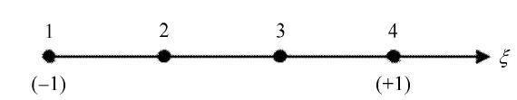
一维问题的拉格朗日插值函数可以表示为[21]$$L_I^ (\xi ) = \prod\limits_{i = 1,i \ne I}^m \dfrac{\xi - \xi _i}{\xi _I - \xi _i } \,, \ \ I = 1 \sim m,\;\; - 1 \leqslant \xi \leqslant 1 (9)$$
其中,$m$为等参坐标(也叫自然坐标)$\xi $的插值点数. 通常,插值点$\xi _i$取区间[-1, 1]之间的等分节点,但本文采用不等间隔单元,使其适应性更强,其中各节点的等参坐标值$\xi_i $由单元相邻节点的距离来确定. 图1为四节点线单元节点分布示意图.
 显示原图|下载原图ZIP|生成PPT
图1四节点一维等参线单元
-->Fig. 1Four-node line element
-->
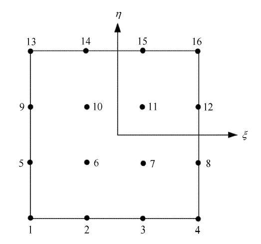
二维问题的拉格朗日形函数可由一维问题的插值函数构成[22]
$$N_\alpha (\xi ,\eta ) = L_I (\xi )L_J (\eta ) (10)$$
其中,下标$\alpha $的值是通过$\xi $方向的指标$I$和$\eta $方向的指标$J$的顺序排列形成的. 图2展示了16节点的二维等参单元节点分布,形函数由式(10)形成,如$N_7 $可以表示为$N_7 \left( {\xi ,\eta } \right) = L_3 \left( \xi \right)L_2 \left( \eta \right)$.
 显示原图|下载原图ZIP|生成PPT
图2十六节点矩形等参单元
-->Fig. 216-node quadrilateral element
-->
2.2 七节点三角形等参单元
拉格朗日单元具有容易构造高阶单元的特点,但对于一些不规则的几何形状采用三角形单元更具灵活性. 为此,作者构造了一种具有一个内部点的七节点二次三角形等参单元(见图3),其形函数见附录.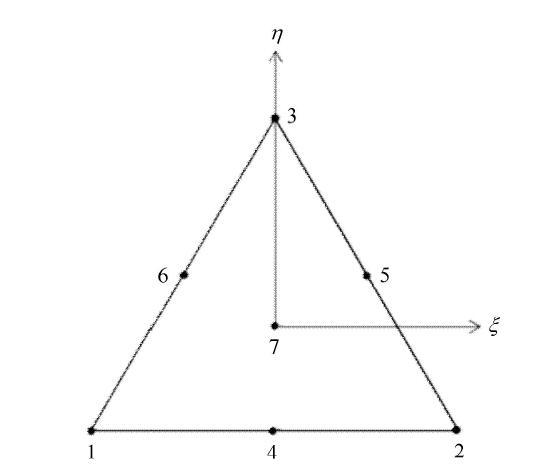 显示原图|下载原图ZIP|生成PPT
图3七节点三角形等参单元
-->Fig. 37-node triangle element
-->
2.3 单元形函数对总体坐标的偏导数计算式
有了上述等参单元形函数,坐标和物理量在一个单元内的变化关系则可由单元结点值来表示$x_i (\xi ,\eta ) = N_\alpha (\xi ,\eta )x_i^\alpha (11)$
$u_i (\xi ,\eta ) = N_\alpha (\xi ,\eta )u_i^\alpha (12)$
其中,$x_i^\alpha $和$u_i^\alpha $分别为单元结点$\alpha $的坐标和位移值,重复指标$\alpha$表示遍及所有单元结点求和. 对式(12)中的位移求偏导数可得[22]
$\dfrac{\partial u_i }{\partial x_j } = \dfrac{\partial N_\alpha }{\partial x_j }u_i^\alpha (13)$
$\dfrac{\partial ^2u_i }{\partial x_k \partial x_l } = \dfrac{\partial ^2N_\alpha }{\partial x_k \partial x_l }u_i^\alpha (14)$
从式(9)和式(10)可以看出,形函数是等参坐标$\xi _k $的显式函数,因此有
$\dfrac{\partial N_\alpha }{\partial x_i } = \dfrac{\partial N_\alpha }{\partial \xi _k }\dfrac{\partial \xi _k }{\partial x_i } = [J]_{ik}^{ - 1} \dfrac{\partial N_\alpha }{\partial \xi _k } (15)$
$\dfrac{\partial ^2N_\alpha }{\partial x_i \partial x_j } = \left[ {[J]_{ik}^{ - 1} \dfrac{\partial ^2N_\alpha }{\partial \xi _k \partial \xi _l } + \dfrac{\partial [J]_{ik}^{ - 1} }{\partial \xi _l }\dfrac{\partial N_\alpha }{\partial \xi _k }} \right]\dfrac{\partial \xi _l }{\partial x_j } (16)$
其中,$[J] = [\partial x / \partial \xi ]$为从总体坐标系到等参坐标系转换的雅可比矩阵.文献[22]导出了式(15)和式(16)中的各项显式计算式.
3 强形式的自由单元法(SFECM)
自由单元法的基本思想是像无网格法一样,将计算域离散成一系列节点,系统方程逐点配置而成.具体思路是,在每个配置点周围自由选择一些节点与其形成一个独立的等参单元(叫做配点单元),此单元是自由的(不与其他单元连接),并由式(13)$\sim$式(16)表达位移对坐标的一阶和二阶偏导数,然后将其直接代入控制方程与纽曼边界条件产生代数方程组.图4给出了采用九节点拉格朗日单元(黑线表示)和五节点十字单元[23](蓝线表示)作为配点单元的示意图.其他类型的等参单元[25]也可以作为配点单元,但对于内部点,为了获得较高的计算精度,需要使用至少有一个内部点的等参单元,以便将配置点放在单元的内部节点上;对于边界节点,可以使用任意形式的等参单元,因为配置点只能放在单元的边界节点上.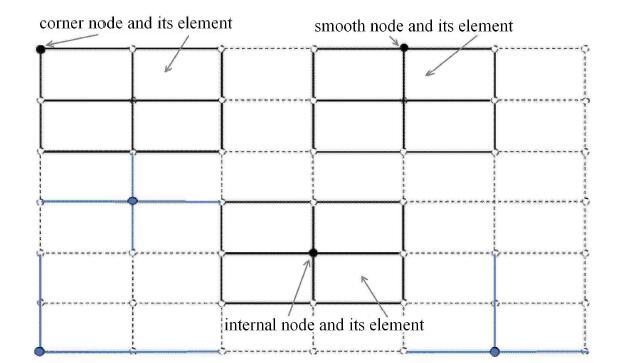 显示原图|下载原图ZIP|生成PPT
图 4配置点及其等参单元示意图
-->Fig. 4Collocation points and isoparametric element diagrams
-->
这样,对于内部点,将微分关系式(14)直接代入控制方程(7)可得到下列方程
$${ D}_{ijkl} \dfrac{\partial ^2N_\alpha ({\pmb \xi} )}{\partial x_j \partial x_l }u_k^\alpha + f_i ({\pmb x})= 0 (17)$$
其中,${\pmb\xi }$表示对应于配置点的单元结点的等参坐标值,${\pmb x}$表示该配置点的总体坐标.
对于边界节点,将式(13)代入面力$\!$-$\!$-$\!$位移关系式(8)可得到下列方程
$$D_{ijkl} \dfrac{\partial N_\alpha ({\pmb \xi })}{\partial x_l }n_j u_k^\alpha ={ t}_i (18)$$
由式(17)和式(18)可见,内部点和边界点的代数方程为由所在单元各节点位移表示的线性方程组. 对所有的节点进行配点,并施加已知的边界条件后,则可建立起形如$AX=b$或$KU=F$的系统方程组(其处理与文献[22]和一般有限元法中的一样). 当所有节点的位移通过求解该系统方程获得后,则可由式(2) $\sim$式(4)和式(13)、式(15)计算各节点的应力值.
4 弱形式的自由单元法(WFECM)
与上述强形式一样,弱形式的自由单元法也是在每个节点采用一个与周围节点自由形成的等参单元. 不同之处是,为了使用高斯积分公式计算积分,所用的自由单元需要是等参变量变化范围为$[-1,+1]$之间的等参单元.这样,对每个配置点(用符号*标记),对控制方程(1)建立如下形式的加权余量积分式$$\int_\varOmega {w\dfrac{\partial \sigma _{ij} }{\partial x_j }\varOmega } + \int_\varOmega {w\,f_i \varOmega } = 0 (19)$$
式中,积分域$\varOmega $为当前自由单元的面积(二维)或体积(三维),$w$为在$\varOmega $内连续的权函数.
对式(19)进行分部积分,并使用高斯散度公式和考虑式(2) $\sim$式(6)则可得到下列积分式
$$ \int_\varGamma {w\,t_j \varGamma } - \int_\varOmega {\dfrac{\partial w}{\partial x_j }D_{ijkl} \dfrac{\partial u_k }{\partial x_l } \varOmega } +\int_\varOmega {w\,f_i \varOmega } = 0 (20) $$
式中,$\varGamma $为积分域$\varOmega $的边界.
在式(20)中,如果取权函数$w$为1,则可得到像有限体积法[9]中那样的算法,但在本文中我们取$w$为式(12)中表示位移变化的形函数$N_\alpha $中对应于配置点的形函数$N_{\ast }$. 这样,使用式(13),由式(20)可得到如下伽辽金形式的积分公式
$$ \int_{\varGamma _{\rm s} } {N_{\ast } N_\beta \varGamma t_j^\beta } - \int_\varOmega {\dfrac{\partial N_{\ast } }{\partial x_j }D_{ijkl} \dfrac{\partial N_\alpha }{\partial x_l } \varOmega } \,u_k^\alpha + \int_\varOmega {N_{\ast } N_\alpha \varOmega } f_i^\alpha = 0 (21) $$
式中,边界积分域$\varGamma _s $为积分单元暴露在整个计算域外边的边界,当配置点为内部点时,该积分为零;指标$\beta $只取积分单元在外边界$\varGamma _{\rm s}$上的节点,$f_i^\alpha $表示体积力$f_i $在第$\alpha$个节点上的值.
需要说明的是,式(21)已考虑了配置点的形函数$N_{\ast }$在不包括其的其他边上的值为零的特性,因此该公式不适用于其他不完备的退化单元,如十字单元[23]和最简单元[25],但拉格朗日单元以及有限元法中的Serendipity单元都适用于该公式.此外,式(21)虽然与传统有限元法的公式在形式上相似,但在本文方法中,一个单元只用于一个节点,不需要与其他单元的结果进行组集,这是主要的不同.
5 数值算例
利用本文所推导的公式,我们编制了FORTRAN程序,并对一些弹性力学问题做了计算分析,用以验证强、弱两种形式方法的正确性.5.1 端部受剪悬臂梁
为了验证算法的精度,这里给出了一个简单的二维平面问题算例. 现考虑一悬臂梁,在其自由端施加一抛物线型面力,模型如图5所示. 按照平面应力求解.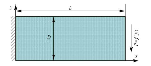 显示原图|下载原图ZIP|生成PPT
图5自由端受剪力的悬臂梁模型
-->Fig. 5Cantilever beam with shear free force at the end
-->
假设右端抛物线型切向载荷满足公式
$$p = \dfrac{Py}{I}(y - D) (22)$$
则可以得到应力解析解为[16]
$$ \left.\begin{array}{l} \sigma _{11} = \dfrac{P}{I}(L - x)\left( {y - \dfrac{D}{2}} \right) \\ \sigma _{22} = 0 \sigma _{12} = \dfrac{Py}{I}(y - D) \end{array} \right \} (23) $$
上两式中,$L$为悬臂梁的长度,$D$为宽度,$I$为惯性矩,对于单位厚度的矩形截面有$I= D^3 / 12$.
在本问题中,梁的弹性模量取为200,GPa,泊松比取为0.3,几何尺寸参数$L = 10$,mm,$D = 4$,mm,右端载荷参数$P =1$,GPa.
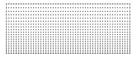
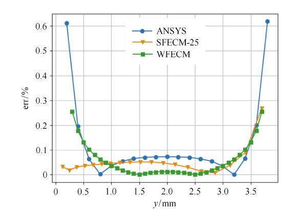
在本算例中,分别采用高阶强形式自由单元法SFECM和低阶弱形式自由单元法WFECM进行计算.对于SFECM模型,整个悬臂梁被离 散成1071个节点,其分布如图6所示. 每个节点与周围的24个节点形成$5\times 5 =25$节点的高阶拉格朗日单元用于计算. 对于弱形式WFECM,这里采用比强形式更密一倍的网格,配点与周围的8个节点形成$3\times 3 = 9$节点的低阶拉格朗日单元.同时采用ANSYS计算并与解析解比较误差. ANSYS所采用单元类型为八节点单元,总单元数1000,总节点数为3141.为了和有限元对比,WFECM采用均匀分布的节点. 经过计算,上的节点比较剪应力分布,得到如图7的误差曲线.
 显示原图|下载原图ZIP|生成PPT
图6悬臂梁计算模型不等间隔节点分布图
-->Fig. 6Nodes distribution over the cantilever beam
-->
 显示原图|下载原图ZIP|生成PPT
图7$x=L/2$线上剪应力的误差曲线
-->Fig. 7Error of shear stress on line of $x=L/2 $
-->
从图7中可以看出,相比较ANSYS,采用弱形式的WFECM误差更小. 对于高阶强形式SFECM其计算误差最小.由此可见SFECM计算的 应力最精确,并且在整条路径上应力误差在较小的范围内变化,说明SFECM计算精度高,稳定性好.
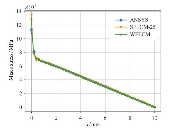
同时,绘制了WFECM,SFECM和ANSYS三种方法所得的底面上的Mises应力和$y$方向位移曲线(如图8和图9所示),并在图10中绘制出了ANSYS和SFECM所得的整体悬臂梁的Mises应力云图.
 显示原图|下载原图ZIP|生成PPT
图8底边上Mises应力曲线图
-->Fig. 8Mises stress curve on the bottom
-->
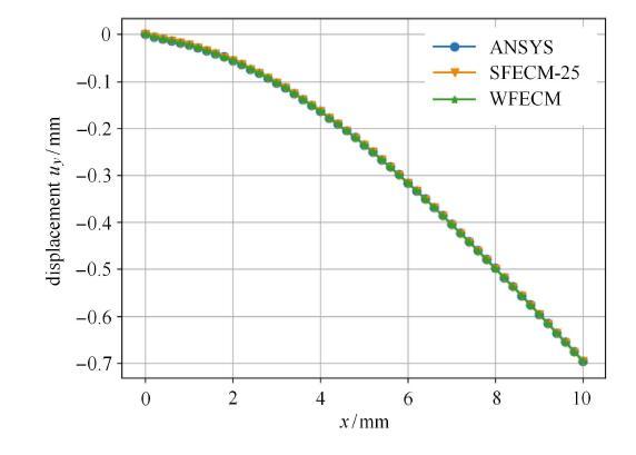 显示原图|下载原图ZIP|生成PPT
图9底面上$y$方向位移曲线图
-->Fig. 9Displacement in $y$-direction on the bottom
-->
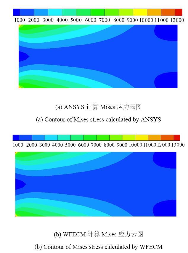 显示原图|下载原图ZIP|生成PPT
图10两种FECM方法计算所得悬臂梁整体Mises应力云图
-->Fig. 10The Mises stress contour of the whole model calculated by two method of FECM respectively
-->
从图8可以看出3种算法所得Misis应力解非常接近,但在固定端,SFECM的解更能体现应力集中现象.这里需要指出,文献中提到的应力解 析解是在$L \gg D$的前提下得到的,其只适用于远离固定端的区域,在固定端的应力解析形式并不满足式(23),因此这里并不给出解析形式的Mises应力云图.
5.2 厚壁圆筒受压分析
本算例分析如图11所示的承受均布内压的厚壁圆筒,内半径$d_1 = 50$\,mm,外半径$d_2 = 100$\,mm,内壁面压强$p =0.4$\,MPa,材料的弹性模量$E$为$2.1$\,TPa,泊松比$\nu $为0.3.因为对称,可取1/4部分计算,FECM所采用的节点分布如图12所示.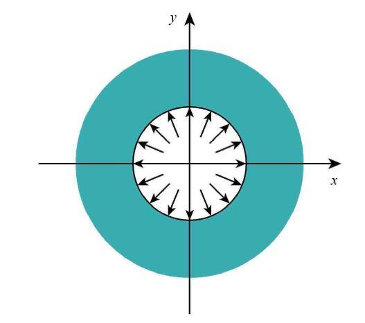 显示原图|下载原图ZIP|生成PPT
图11受内压的厚壁圆筒
-->Fig. 11Thick-walled cylinder under inner pressure
-->
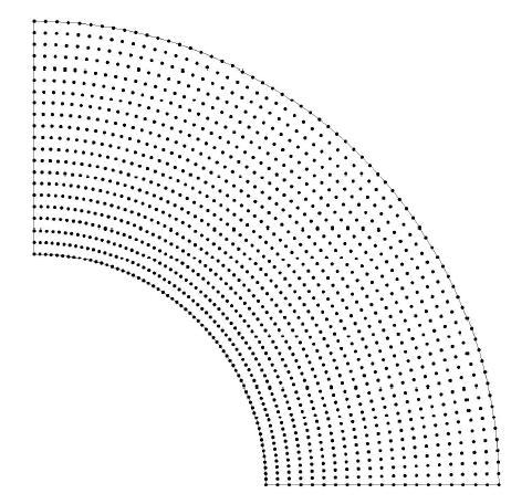 显示原图|下载原图ZIP|生成PPT
图12圆筒节点分布
-->Fig. 12Distribution of nodes over the thick-walled cylinder
-->
此问题的位移和应力解析解可求得为[27]
$u_r = \dfrac{1}{E}\dfrac{d_1^2 p}{d_2^2 - d_1^2 }\left[ {(1 + \nu )\dfrac{d_2^2 }{r} + (1 - \nu )r} \right] (24)$
$ \sigma _r = - \dfrac{\dfrac{d_2^2 }{r^2} - 1}{\dfrac{d_2^2 }{d_1^2 } - 1}p\,,\quad \sigma _\theta = \dfrac{\dfrac{d_2^2 }{r^2} + 1}{\dfrac{d_2^2 }{d_1^2 } - 1}p (25)$
对于本问题,FECM采用3种方式进行计算,即分别采用九节点、二十五节点单元的强形式(SFECM)以及九节点单元的弱形式(WFECM).3种方式采用如图12所示的同一套节点网格,其总节点数为1365.为了比较,同时使用有限元软件ANSYS进行计算,其采用八节点等参单元,总节点数为1045.
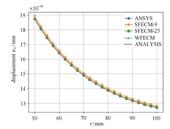
我们取1/4模型的底部,即路径$y=0$上的节点进行比较,位移变化如图13所示.从图13可以看出,使用高阶强形式和低阶弱形式所得 的结果和解析解十分相近.
 显示原图|下载原图ZIP|生成PPT
图13圆筒径向位移曲线图
-->Fig. 13Displacement distribution along radial direction
-->
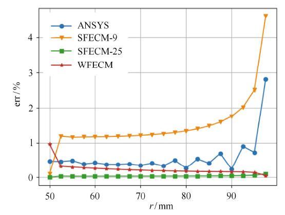
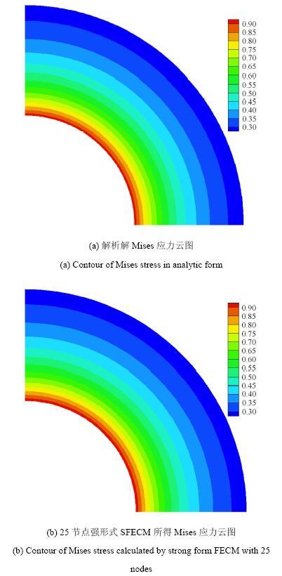
图14给出了ANSYS和3种FECM模型计算所得的径向应力$\sigma _r$的误差曲线,从图中可以看出,对于此密度的节点分布模型,九节点低阶单元强形式模型SFECM-9并不能得到较高的精度,但使用二十五节点高阶单元强形式模型SFECM-25可以得到十分精确的计算结果,同样九节点弱形式算法WFECM可以得到较高的精度.从图14也可以看出,高阶强形式和低阶弱形式的自由单元法计算精度都高于ANSYS的计算精度.图15给出了解析形式的及二十五节点强形式SFECM-25模型计算所得的Mises应力云图.对于弱形式WFECM和九节点强形式SFECM-9的计算结果和其类似.
 显示原图|下载原图ZIP|生成PPT
图14沿径向的应力$\sigma _r $误差曲线图
-->Fig. 14Error of $\sigma _r $ along radial direction
-->
 显示原图|下载原图ZIP|生成PPT
图15圆筒的Mises应力云图
-->Fig. 15Mises stress contour of the cylinder
-->
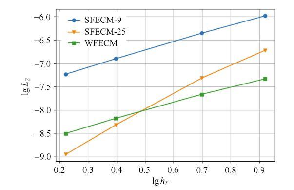
为了验证本文算法的网格收敛性,针对本算例我们又对另外3种不同节点密度的模型进行了计算,其节点数分别为112,363和3007. 图16给出了$L_2 $误差范数随单元平均尺寸的变化曲线. $L_2$误差范数的变化能体现计算方法的整体收敛性,其定义为$L_2 = \sqrt {(u - \mathop{u}\limits^{\_}) \cdot (u -\mathop{u}\limits^{\_}) / n} $,其中$u$和$\bar{u}$分别为计算所得的各节点位移矢量和解析解位移矢量,$n$为模型的总节点数.从图16可以看出,计算结果的整体收敛性很好,表明本文算法具有良好的稳定性.
 显示原图|下载原图ZIP|生成PPT
图16$L_2$ 误差范数随单元尺寸的变化曲线
-->Fig. 16The curve of L2 norm versus element size
-->
5.3 对称边界的带圆孔复合圆弧
以上两算例模型中均是采用结构化(拉格朗日)单元,本算例将讨论具有非结构化(七节点)单元的情形.如图17所示为一受内压带圆孔 复合圆弧,外半径$R = 100$,内半径$r = 60$,其内部圆孔的直径$d = 10$.所受边界条件与上一算例类似,两端为对称边界条件,内壁面压强$p = 1000$. 材料的弹性模量$E$为$2\times10^5$,泊松比$\nu $为0.3. 按平面应力分析.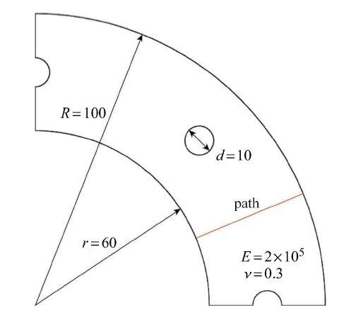 显示原图|下载原图ZIP|生成PPT
图17受内压带圆孔复合圆弧
-->Fig. 17Composite circular arch with circular holes under inner pressure
-->
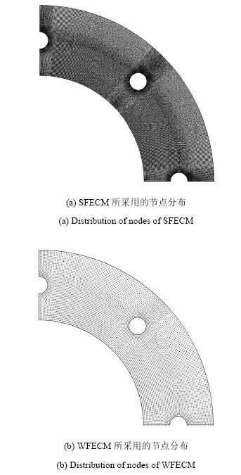
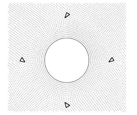
分别采用本文所提到的两种FECM方法进行计算. 由于目前还没有此问题的解析解,因此需要使用ANSYS进行计算对比.对于SFECM,由于问题的复杂性,采用较密节点分布并使用二十五节点高阶单元,由于模型中有些点处生成拉格朗日单元是不便的,因此在这些位置采用七节点三角形单元. 对于WFECM,仍采用九节点拉格朗日单元,所采用网格密度和ANSYS类似.图18中给出了两种FECM的网格分布. 图19中给出了SFECM中所使用的几个七节点三角形单元的具体形成方式.同样,对于模型中另外两个圆孔周围也有这种单元分布,在这里仅给出中间圆孔周围的单元形式.本算例的两种模型总节点数分别为30,368和7,728,ANSYS为22,020.
 显示原图|下载原图ZIP|生成PPT
图18两种FECM所采用的节点分布
-->Fig. 18The nodes distribution of two method of FECM
-->
 显示原图|下载原图ZIP|生成PPT
图19中间圆孔周围的三角形单元组成形式
-->Fig. 19Triangular elements around a circular hole in the middle of the model
-->
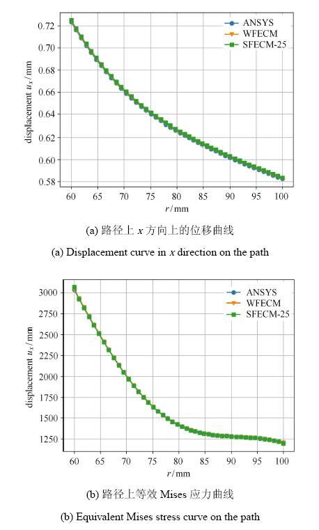
比较如图 17中红线上节点处的位移值和应力值.在图20中给出了3种方法所得的位移$u_{x}$和等效Mises应力曲线,经过比较 发现3种方法所得结果十分接近.
 显示原图|下载原图ZIP|生成PPT
图 203种方法计算所得路径上的位移和应力值
-->Fig.20The value of displacement and stress on the path calculated by three methods respectively
-->
本算例验证了对于复杂几何外形,无论是强形式还是弱形式,本文方法均可以得到精确的结果.
本算例还验证了七节点三角形单元的准确性,发现在较难生成拉格朗日单元的位置,可使用三角形单元,而且仍得到十分精确的结果.
6 结论与讨论
本文介绍了强形式与弱形式两种自由单元法,用数值算例验证了其正确性与有效性,可得出下列结论:(1) 自由单元法是一种单元配点法,对每个节点只需要一个独立的自由形成的局部单元进行配点,具有建模方便和容易实施并行计算的优点.
(2) 由于自由单元法只需要一个单元配点,因此对于内部点,为了获得较高的计算精度,所用的等参单元至少要有一个内部点(用于配点).
(3) 强形式的自由单元法,直接由控制方程和边界条件建立系统方程组,便于建立多物理场耦合问题的统一求解格式;可用任意形式的等参变量建立单元节点形函数,并可选用任意形式的等参单元. 缺点是,由于直接由控制方程配点要用到单元的二阶偏导数,因此需要至少二次的等参单元,如果要想获得较高的计算精度并要求节点数不要太多,则需要使用高次单元.
(4) 弱形式的自由单元法,由于通过了一次积分,只用到了单元的一阶偏导数,因此,采用同样阶次的等参单元,计算精度要比强形式的高.缺点是,对于不是全微分形式(守恒形式)的控制方程,则不易将其进行分部积分,较难建立多场耦合问题的统一求解格式.此外,由于要用到单元积分,因此所用的单元形函数,需要用从$-1$到$+1$的参变量来表征.
(5) 因为每个节点使用其独立的等参单元,不难想象全部节点的等参单元将形成互相重叠的网格,这对结果的显示会带来一定的不便.
(6) 尽管本文以二维弹性力学问题作为研究对象,但其方法和所推导的公式很容易推广到其它类型的问题.
附录
七节点三角形等参单元形函数$N_1 (\xi ,\eta ) = \dfrac{1}{18}\xi \Big [ - 3 + \sqrt 3 + 3\xi - 3\eta (1 - 2\sqrt 3 + 2\sqrt 3 \eta + 2\sqrt 3 \xi )\Big ] $
$N_2 (\xi ,\eta ) = \dfrac{1}{18}\xi \Big [ 3 + \sqrt 3 + 3\xi - 3\eta (1 + 2\sqrt 3 + 2\sqrt 3 \eta + 2\sqrt 3 \xi ) \Big ] $
$ N_3 (\xi ,\eta ) = \dfrac{1}{18}\Big [ 3\eta (\sqrt 3 + 3\eta ) + \sqrt 3 \xi- 3\eta (1 + 2\sqrt 3 \eta )\xi - 6(1 + \sqrt 3 \eta )\xi ^2\Big ] $
$ N_4 (\xi ,\eta ) = \dfrac{1}{9}\Big [\xi ( - 2\sqrt 3 + 3\xi )+ 3\eta ^2(3 + 4\sqrt 3 \xi ) + 6\eta ( - \sqrt 3 + \xi + 2\sqrt 3 \xi ^2) \Big ] $
$ \begin{array}{l} N_5 (\xi ,\eta ) = \dfrac{2}{9}\xi \Big [3 - \sqrt 3 + 6\xi + 3\eta (1 + \sqrt 3 + 2\sqrt 3 \eta + 2\sqrt 3 \xi ) \Big ] \end{array} $
$ \begin{array}{l} N_6 (\xi ,\eta ) = \dfrac{2}{9}\xi \Big [ - 3 - \sqrt 3 + 6\xi + 3\eta (1 - \sqrt 3 + 2\sqrt 3 \eta + 2\sqrt 3 \xi ) \Big ] \end{array} $
$ \begin{array}{l} N_7 (\xi ,\eta ) = \dfrac{1}{2}(2 + \Big [\sqrt 3 - 3\eta )\eta + \sqrt 3 \xi - 3\eta (1 + 2\sqrt 3 \eta )\xi - 6(1 + \sqrt 3 \eta )\xi ^2\Big ] \end{array} $
The authors have declared that no competing interests exist.
参考文献 原文顺序
文献年度倒序
文中引用次数倒序
被引期刊影响因子
| [1] | |
| [2] | |
| [3] | |
| [4] | Least-squares 03nite element methods are an attractive class of methods for the numerical solution of partial differential equations. They are motivated by the desire to recover, in general settings, the advantageous features of Rayleigh–Ritz methods such as the avoidance of discrete compatibility conditions and the production of symmetric and positive de03nite discrete systems. The methods are based on the minimization of convex functionals that are constructed from equation residuals. This paper focuses on theoretical and practical aspects of least-square 03nite element methods and includes discussions of what issues enter into their construction, analysis, and performance. It also includes a discussion of some open problems. |
| [5] | . Presented modification of the FDM enables local condensation of the mesh and easy discretisation of the boundary conditions in the case of an arbitrary shape of the domain. As a result an essential reduction of the required number of nodal points may usually be achieved. Thus the FDM can be competitive in some fields to the finite element method. Several troubles arising from the use of an irregulr mesh have been solved, the most important being elimination of singular or ill-conditioned stars, and a successful way of automatic discretization of boundary conditions was proposed. As a result of this complete automatization of the FDM has been reached. Many problems connected with the theory of the method proposed and its computer implementation have been discussed. FIDAM code鈥攁 system of computer programs designed for the solution of two-dimensional, linear and nonlinear, elliptic problems and three-dimensional parabolic problems is presented. Problems to be solved should be layed down in a local formulation as a set of partial derivative equations of the second order with boundary conditions not exceeding the same order. Various particular problems of applied mechanics and physics such as: torsion of bars, plane elasticity problems, deflections of plates and membranes, fluid now and temperature distribution have been solved using the FIDAM procedures. For the solution of nonlinear problems various iterative methods have been adopted鈥攚ith special attention payed to the self-correcting method where the Newton-Raphson and incremental procedures are particular cases. The present version of the method allows fully automatic calculations to be carried out as in advanced programs of the finite element method and may be preferred in non-linear, optimization and time-dependent problems. |
| [6] | . Partial differential equation problems arising in contemporary engineering problems are often solved numerically using finite difference techniques. The majority of the attention has been devoted to the rectangular grid formulation. The complications of applying rectangular grids on curved boundaries, however, has motivated active study of finite difference methods using non-rectangular grids since about 1953. The majority of the effort on variable grid techniques appears to have been directed toward the solution of self adjoint systems using an energy formulation. A hexagonal mesh element is generally used in these approaches. Another approach which has received minimal attention is finite difference evaluation on an arbitrary grid using, e.g. two dimensional Taylor expansion. The truncation error using this approach can be rigorously shown to converge to zero with increasing nodal density. There appear to be two pitfalls in the practical application of this approach, namely; (1) how to select a set of neighboring nodes for a given node to use for the finite difference evaluation and (2) how to efficiently handle the vast number of difference coefficients that can result from a given grid. Fortunately neither of these problems is insurmountable. Preliminary studies indicate that for many shell problems this variable grid technique will yield improved efficiency as well as a simple method for handling curved boundaries and varying stress patterns. |
| [7] | . A radial point interpolation based finite difference method (RFDM) is proposed in this paper. In this novel method, radial point interpolation using local irregular nodes is used together with the conventional finite difference procedure to achieve both the adaptivity to irregular domain and the stability in the solution that is often encountered in the collocation methods. A least-square technique is adopted, which leads to a system matrix with good properties such as symmetry and positive definiteness. Several numerical examples are presented to demonstrate the accuracy and stability of the RFDM for problems with complex shapes and regular and extremely irregular nodes. The results are examined in detail in comparison with other numerical approaches such as the radial point collocation method that uses local nodes, conventional finite difference and finite element methods. Copyright 漏 2006 John Wiley & Sons, Ltd. |
| [8] | . In this paper, we present two higher-order compact finite difference schemes for solving one-dimensional (1D) heat conduction equations with Dirichlet and Neumann boundary conditions, respectively. In particular, we delicately adjust the location of the interior grid point that is next to the boundary so that the Dirichlet or Neumann boundary condition can be applied directly without discretization, and at the same time, the fifth or sixth-order compact finite difference approximations at the grid point can be obtained. On the other hand, an eighth-order compact finite difference approximation is employed for the spatial derivative at other interior grid points. Combined with the Crank-Nicholson finite difference method and Richardson extrapolation, the overall scheme can be unconditionally stable and provides much more accurate numerical solutions. Numerical errors and convergence rates of these two schemes are tested by two examples. (C) 2013 Elsevier Inc. All rights reserved. |
| [9] | . Numerical simulations were conducted to reveal the inherent relation between the filed synergy principle and the three existing mechanisms for enhancing single phase convective heat transfer. It is found that the three mechanisms, i.e., the decreasing of thermal boundary layer, the increasing of flow interruption and the increasing of velocity gradient near a solid wall, all lead to the reduction of intersection angle between velocity and temperature gradient. It is also revealed that at low flow speed, the fin attached a tube not only increases heat transfer surface but also greatly improves the synergy between the velocity and the temperature gradient. |
| [10] | . A method is presented for representing curved boundaries for the solution of the Navier–Stokes equations on a non-uniform, staggered, three-dimensional Cartesian grid. The approach involves truncating the Cartesian cells at the boundary surface to create new cells which conform to the shape of the surface. We discuss in some detail the problems unique to the development of a cut cell method on a staggered grid. Methods for calculating the fluxes through the boundary cell faces, for representing pressure forces and for calculating the wall shear stress are derived and it is verified that the new scheme retains second-order accuracy in space. In addition, a novel “cell-linking” method is developed which overcomes problems associated with the creation of small cells while avoiding the complexities involved with other cell-merging approaches. Techniques are presented for generating the geometric information required for the scheme based on the representation of the boundaries as quadric surfaces. The new method is tested for flow through a channel placed oblique to the grid and flow past a cylinder at Re=40 and is shown to give significant improvement over a staircase boundary formulation. Finally, it is used to calculate unsteady flow past a hemispheric protuberance on a plate at a Reynolds number of 800. Good agreement is obtained with experimental results for this flow. |
| [11] | . A series of experimental investigations of boiling incipience and bubble dynamics of water under pulsed heating conditions for various pulse durations ranging from 1 ms to 100 ms were conducted. Using a very smooth square platinum microheater, 100 渭m on a side, and a high-speed digital camera, the boiling incipience was observed and investigated as a function of the bulk temperature of the microheater, pulse power level, and pulse duration. Given a specific pulse duration, for low pulse power levels, there would be no bubble nucleation or bubble mergence, for moderate pulse power levels, individual bubbles generated on the heater merged to form a single large bubble, while for high pulse power levels, the rapid growth of the individual bubbles and subsequent bubble interaction, resulted in a reduction in bubble coalescence into a single larger bubble, referred to as bubble splash. The transient heat flux range at which bubble coalescence occurs was identified experimentally, along with the temporal variations of bubble size, bubble interface velocity and interface acceleration. |
| [12] | . |
| [13] | |
| [14] | . Reliable computational techniques are developed for the solution of two-dimensional (2-d) transient heat conduction problems in anisotropic media with continuously variable material coefficients. Two kinds of the domain-type interpolation, namely the standard domain elements and the meshless point interpolation, are adopted for the approximation of the spatial variation of the temperature field or its Laplace-transform. The coupling among the nodal values of the approximated field is given by integral equations considered on local sub-domains. Three kinds of local integral equations are derived from physical principles instead of using a weak-form formulation. The accuracy and the convergence of the proposed techniques are tested by several examples and compared with exact benchmark solutions, which are derived too. |
| [15] | . In this paper, a new boundary-domain integral equation for solving energy equation in convective heat transfer problems is derived. The derived integral equation accounts for fluid velocity which is computed using the velocity boundary-domain integral equations presented in [2,3] (X.W. Gao, 2004, 2005). Numerical implementation of these integral equations is discussed for steady incompressible fluid flows, in which the velocity and pressure integral equations are uncoupled from the temperature equation, and thus can be solved separately. By substituting the velocity, velocity gradient, and pressure integral equations into the energy integral equation, temperatures can be computed without iterative processes. Two numerical examples for 2D problems are given to validate the proposed method. (C) 2013 Elsevier Ltd. All rights reserved. |
| [16] | . |
| [17] | |
| [18] | . An efficient nesting sub-domain gradient smoothing integration algorithm is proposed for Galerkin meshfree methods with particular reference to the quadratic exactness. This approach is consistently built upon the smoothed gradients of meshfree shape functions defined on two-level nesting triangular sub-domains, where each integration cell consists of four equal-area nesting sub-domains. First, a rational measure is designed to evaluate the error of the gradient smoothing integration for the stiffness matrix. Thereafter through a detailed analysis of the gradient smoothing integration errors associated with the two-level nesting triangular sub-domains, a quadratically exact algorithm for the stiffness matrix integration is established through optimally combining the contributions from the two-level nesting sub-domains. Meanwhile, the integration of force terms consistent with the stiffness integration is presented in order to ensure exact quadratic solutions within the Galerkin formulation. It is noted that the proposed approach with quadratic exactness shares the same foundation as the well-established stabilized conforming nodal integration method with linear exactness, i.e., the smoothed derivatives of meshfree shape functions are directly built upon the values of meshfree shape functions on the boundary of the integration cells and the time consuming derivative computations are completely avoided. Moreover, the present formulation has even less integration sampling points than the four point Gauss integration. Numerical examples show very favorable performance regarding the accuracy and efficiency for the proposed approach. |
| [19] | . Meshless methods for solving differential equations have become a promising alternative to the finite element and boundary element methods. In this paper, an improved meshless collocation method is presented for use with either moving least square (MLS) or compactly supported radial basis functions (RBFs). A new technique referred to as an indirect derivative method is developed and compared with the direct derivative technique used for evaluation of second-order derivatives and higher-order derivatives of the MLS and RBF shape functions at the field point. As the derivatives are obtained from a local approximation (MLS or compact support RBFs), the new method is computationally economical and efficient. Neither the connectivity of mesh in the domain/boundary nor integrations with fundamental/particular solutions is required in this approach. The accuracy of the two techniques to determine the second-order derivative of shape function is assessed. The applications of meshless method to two-dimensional elastostatic and elastodynamic problems have been presented and comparisons have been made with benchmark analytical solutions. Copyright 脗漏 2007 John Wiley & Sons, Ltd. |
| [20] | . In this paper a meshless method of lines is proposed for the numerical solution of time-dependent nonlinear coupled partial differential equations. Contrary to mesh oriented methods of lines using the finite-difference and finite element methods to approximate spatial derivatives, this new technique does not require a mesh in the problem domain, and a set of scattered nodes provided by initial data is required for the solution of the problem using some radial basis functions. Accuracy of the method is assessed in terms of the error norms L2, L鈭 and the three invariants C1, C2, C3. Numerical experiments are performed to demonstrate the accuracy and easy implementation of this method for the three classes of time-dependent nonlinear coupled partial differential equations. |
| [21] | . |
| [22] | . react-text: 116 This paper presents a fast multipole accelerated singular boundary method (SBM) to the solution of the large-scale three-dimensional Helmholtz equation at low frequency. By using a desingularization strategy to directly compute singular kernels in the strong-form collocation discretization, the SBM formulations are derived for the Dirichlet and Neumann problems. A fast multipole method (FMM)... /react-text react-text: 117 /react-text [Show full abstract] |
| [23] | |
| [24] | . |
| [25] | |
| [26] | . . |
| [27] | . |
