基于分布式感知深度神经网络的高分辨率PM2.5值估算

删除或更新信息，请邮件至freekaoyan#163.com(#换成@)

本站小编 Free考研考试/2021-12-29

刘基伟^,, 闵素芹, 金梦迪中国传媒大学数据科学与智能媒体学院,北京 100024

High resolution PM_2.5 estimation based on the distributed perception deep neural network model

LIU Jiwei^,, MIN Suqin, JIN MengdiCollege of Data Science and Intelligent Media, Communication University of China, Beijing 100024, China

收稿日期:2019-12-2修回日期:2020-11-3网络出版日期:2021-01-25

基金资助:

中央高校基本科研业务费专项资金.3132018XNG1830

Received:2019-12-2Revised:2020-11-3Online:2021-01-25

Fund supported:

The Fundamental Research Funds for The Central Universities of China.3132018XNG1830

作者简介 About authors
刘基伟(1994-), 山东青岛人, 硕士生, 研究方向为统计与计量方法。E-mail: liujiwei@cuc.edu.cn

摘要
细颗粒物（PM_2.5）个体暴露水平是健康效应研究中的关键问题,然而历史数据缺失和地面监测点覆盖范围小阻碍了相关研究。基于美国国家航空航天局遥感数据提供的气溶胶光学厚度（AOD）,融合地面监测、气象等多源数据进行建模来估算近地面PM_2.5浓度,所得结果的空间覆盖范围广、时间连续性强、方法成本低。本文基于2018年京津冀鲁地区,引入气象、NDVI、时间节点、空间标识等50个特征分析AOD-PM_2.5关系。鉴于传统插补方法单一所造成的信息损失,运用时空多视图插补方法来提高插补的精度和广度。考虑到特征的滞后作用、特征间相关性与偏相关性所导致的复杂关系,运用分布式感知深度神经网络模型来分别捕捉多源特征间的高阶特性。结果表明：① 时空多视图插补方法的相对误差为27.5%,数据平均缺失52.1%降至4.84%。② 分布式感知深度神经网络模型在时间预测上平均绝对误差、相对误差、均方误差、均方根误差分别为17.7 μg/m ³、46.8%、766.2 μg ²/m ⁶、26.9 μg/m ³,空间上,为16.6 μg/m ³、41.8%、691.5 μg ²/m ⁶、26.6 μg/m ³,从精度、稳健性、泛化能力和耗时方面综合来看,结果优于线性统计模型和常见深度学习架构。
关键词： 气溶胶光学厚度;PM_2.5;多视图插补;分布式感知;深度学习;时空迁移预测

Abstract

The individual exposure level of fine particulate matter (PM_2.5) is a key issue in the study of health effects. However, the lack of historical data and the small coverage of ground monitoring stations have hindered the development of related research. Based on the aerosol optical depth (AOD) provided by NASA remote sensing data, multi-source data such as ground monitoring and meteorological data were integrated for modeling to estimate near-ground PM_2.5 concentration. The results have wide spatial coverage, strong time continuity and low method cost. Based on the Beijing-Tianjin-Hebei-Shandong region in 2018, this paper introduces 50 features such as meteorological elements, NDVI, time nodes and spatial markers to analyze the relationship between AOD and PM_2.5. In view of the information loss caused by the single traditional interpolation method, the spatiotemporal multi-view interpolation method is used to improve the accuracy and coverage of interpolation. Considering the complex relationship caused by hysteresis of features, and the correlation and partial correlation between features, this paper uses a distributed perception deep neural network model (DP-DNN) to separately capture higher-order features between multiple-source features. The results show that: (1) The relative error of the spatiotemporal multi-view interpolation method is 27.5%, and the average proportion of missing data decreases from 52.1% to 4.84%. (2) In terms of time prediction, mean absolute error, relative error, mean square error and root mean square error of DP-DNN are 7.7 μg/m ³, 46.8%, 766.2 μg ²/m ⁶ and 26.9 μg/m ³, respectively. In terms of space prediction, they are 16.6 μg/m ³, 41.8%, 691.5 μg ²/m ⁶ and 26.6 μg/m ³, respectively. In aspects of accuracy, robustness, generalization ability and time consuming, the results are superior to linear statistical models and common deep learning architecture.

Keywords：aerosol optical depth (AOD);PM_2.5 prediction;multi-view interpolation;distributed perception;deep learning;prediction of spatiotemporal migration

PDF (3098KB)元数据多维度评价相关文章导出EndNote|Ris|Bibtex 收藏本文
本文引用格式
刘基伟, 闵素芹, 金梦迪. 基于分布式感知深度神经网络的高分辨率PM_2.5值估算. 地理学报[J], 2021, 76(1): 191-205 doi:10.11821/dlxb202101015
LIU Jiwei, MIN Suqin, JIN Mengdi. High resolution PM_2.5 estimation based on the distributed perception deep neural network model. Acta Geographica Sinice[J], 2021, 76(1): 191-205 doi:10.11821/dlxb202101015

1 引言

大气细颗粒物（PM_2.5）粒径小且能作毒性物质载体,长期暴露于细颗粒物污染之下的人们更可能面临心血管病和呼吸系统疾病的严重风险。流行病学和健康评估研究中,细颗粒物的危害研究需要长期且空间连续的地面细颗粒物的数据^[1,2,3]。然而,中国2012年底才初步建成PM_2.5地面监测网络,2013年官方数据开始发布;且由于地面监测系统维护费用高,最初几年监测点有限,主要集中在大城市,缺乏历史和空间分辨率高的监测数据,细颗粒物对慢性病的长期健康效应研究相对薄弱。因此,通过其他数据来源估算PM_2.5浓度值具有重要的研究意义和应用价值。

基于卫星遥感监测地面颗粒物能很好弥补地面观测站点的不足。与2013年才开始发布的地面监测数据相比,遥感数据始于1999年,可以提供较为长期的数据;且全球覆盖、空间分辨率高、成本低,更有利于研究PM_2.5的传播趋势。但遥感数据反演得到的气溶胶光学厚度（Aerosol Optical Depth, AOD）是气溶胶消光系数的垂直积分,它是与地面监测完全不同的一种测度空气颗粒物含量的方式,反演的AOD不能直接作为地面PM_2.5浓度估计值。基于AOD遥感数据与PM_2.5浓度测量数据,通过建立区域内或区域间PM_2.5浓度的时空模型,能够有效估算PM_2.5浓度值,提高监测能力^[4,5,6]。

早期研究使用AOD与PM_2.5之间的一元线性回归模型^[7,8,9,10],然而由于气象条件变化的影响,通过引入气象特征,多元线性回归模型可以更准确地表示AOD-PM_2.5的关系^{[11,12,13,14]}。考虑到AOD-PM_2.5关系的空间异质性,地理加权模型和时空地理加权模型被用于估计PM_2.5浓度^{[5, 15-19]},这类模型采用局部回归方法预测PM_2.5浓度,而不是全局常量回归参数。随着研究的深入,AOD-PM_2.5关系逐步被认为是多变量且非线性的关系^[20,21]。因此许多非线性统计模型被用来估计PM_2.5浓度,包括支持向量回归^[22]、随机森林模型^[22],广义加性模型^[23,24,25]、人工神经网络模型以及深度学习方法^{[22, 26-29]}。研究表明,深度神经网络具有更优秀的性能,模型结构更能反映出大气环境系统中的复杂关系。而且,随着模型信息处理效率的提高,更多的特征——气象、土地利用、NDVI以及人口密度特征——被纳入模型^{[11,12,13,14,15,16,17,18,19]}。虽然深度神经网络通过数据信息挖掘,在克服维数灾难上具有先天优势,但现有研究的应用中都忽略了输入特征自相关性（如滞后影响）、特征间相关性、偏相关性和交互作用^[30,31],在特征输入时一同输入,不区分主辅特征,不能够充分的捕获数据蕴含的信息,因此建立能够分别捕捉这类特性的多模块神经网络是必要的。

研究中的缺失数据插补方法多集中于反距离加权插值法^[32,33]、克里金插值法^[34,35]、线性及线性拟合插值法^{[4, 8]},在操作时仅使用单一的插补方法,部分研究仅仅只对有完整观测数据的样本进行了回归^{[11-12, 36]},也缺少对插补效果评估。研究发现PM_2.5浓度不仅存在显著的季节性变化,还存在着明显的地理空间异质性和空间依赖性^{[37,38,39,40,41,42]};其次,缺失发生的时间点和位置也是随机的,从而导致单一方法难以同时地、有效地处理点、条、块状缺失。因此,插补时为有效利用有限信息,降低插补误差,建立综合性的插补方法是必要的。

鉴于此,本文以京津冀鲁地区为研究对象,以气溶胶光学厚度为主要特征,引入气象、归一化植被指数等辅助特征,提出时空多视图插补模型,提升插补效率;运用分布式感知深度神经网络模型（Distributed Perception Deep Neural Network Model, DP-DNN）,捕捉每一种辅助特征和主要特征的复杂关系并学习特征之间的高阶特性从而进一步提高卫星遥感估值近地面PM_2.5浓度的能力。模型能够估值选定经纬度上的近地面PM_2.5浓度,实现时间空间的预测和迁移,从而可以对污染物历史数据进行补全、对未建立监测点的欠发达地区或复杂地面结构区域进行PM_2.5浓度估值。

2 研究方法与数据来源

2.1 数据资料来源和时空匹配准则

2.1.1 多源数据资料的特征选用本文选用了共计50个特征进行京津冀鲁地区的AOD与PM_2.5浓度之间的日差异分析。表1展示了输出、输入特征。本文选用PM_2.5特征作为输出特征;选用AOD特征作为主要输入特征;选用NDVI、气象、时滞、空间标识、时间节点等特征作为辅助输入特征。

Tab. 1
表1
表12018年京津冀鲁地区所用特征
Tab. 1Feature used in the Beijing-Tianjin-Hebei-Shandong region

类别	特征	单位	特征描述
PM_2.5特征	PM_2.5	μg/m³	近地面细颗粒物空气动力学粒径小于等于2.5 μm的颗粒物质量浓度的全日平均值
AOD特征	AOD		MODIS暗像元与深蓝算法融合提取0.55 μm处气溶胶光学厚度
NDVI特征	NDVI		MODIS近红外波段反射值与红光波段反射值之差比上两者之和
气象特征	温度	℃	近地面空气气温的全日平均值
	体感温度^[43]	℃	人体所感受到的冷暖程度,转换成同等温度的全日平均值
	温差	℃	给定日期内近地面空气气温最大温差
	日间温差	℃	给定日期内白天时段近地面空气气温最大温差
	体感温差	℃	给定日期内体感气温最大温差
	日间体感温差	℃	给定日期内白天时段体感气温最大温差
	云量		介于0和之间1的被云遮挡的天空百分比的全日平均值
	露点	℃	空气中所含的气态水达到饱和而凝结成液态水所需要降至的温度的全日平均值
	相对湿度		近地面相对湿度的全日平均值
	日照长度	h	给定日期的日照长度
	能见度	km	平均能见度的全日平均值
	阵风速度	m/s	近地面的阵风速度的全日平均值
	风速	m/s	近地面的风速的全日平均值
	风速角	°	以角度为单位的风的来向,取全日平均风向
	气压	hPa	面积上从海平面到大气上界空气柱的重量的全日平均值
	积雪强度	cm	积雪强度的全日平均值
	降雨强度	cm/h	降雨强度的全日平均值
时滞特征			滞后一日的气溶胶光学厚度、气温、云量、露点、相对湿度、日照长度、能见度、风速、气压、积雪强度、降雨强度
空间标识	经纬度		监测点站点经纬度
时间节点	月份		给定日期所在月份

新窗口打开|下载CSV

2.1.2 多数据资料来源

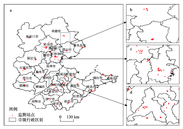
（1）研究区域概况：京津冀鲁地处环渤海区域,位于34°22′N~42°40′N、113°27′E~122°42′E之间,约占全国面积的3.97%,属于温带大陆性季风气候,包含39个城市,建设有152个国家空气环境质量自动监测点。随着京津冀鲁城市群的建设和环渤海经济圈的发展,该地区的地貌环境和城区人类活动发生变化,空气质量受到影响,为更好的反应PM_2.5浓度空间分布及其对人类健康的影响,有必要对该地区可吸入颗粒物进行全范围的监测。

（2）研究时段：数据源于2018年1月1日—2018年12月31日。

（3）地基监测PM_2.5浓度数据：所用的PM_2.5浓度实测数据来源于全国城市空气质量实时发布平台,共获取京津冀鲁地区152个国家空气环境质量自动监测点的每日空气质量数据,图1为研究区范围和152个监测点的分布位置,其中北京市12个、天津市14个、河北省52个、山东省74个监测点。

图1

新窗口打开|下载原图ZIP|生成PPT
图12018年京津冀鲁空气环境质量监测点分布图

Fig. 1Location of air quality monitoring points of Beijing-Tianjin-Hebei-Shandong region in 2018

（4）MODIS AOD数据：Terra/Aqua MODIS 3 km C6.1版本Level 2 AOD产品从NASA网站下载（https://ladsweb.modaps.eosdis.nasa.gov/search/）。C6.1版本较C6版本^[44]优化了深蓝、暗像元算法,修复了算法缺陷;同时开发了新的表面反射模型,消除了系统偏差,提高了对高海拔、崎岖、烟雾地区的预测精度。本文收集了覆盖研究区域的MODIS 3 km C6.1版本Level 2 AOD产品,提取京津冀鲁地区波长为0.55 μm的AOD用于本研究。

（5）气象特征：数据来自气象网站DarkSky,空间分辨率0.25°×0.25°。经由Python API接口即可调用选定经纬度的近地面气象数据,选定的经纬度坐标可以精细到小数点后四位,调用返回的数据值是选定经纬度周围网格的插值。该网站数据源^[45]包括美国NCEP（National Centers for Environmental Prediction）等13个数据来源,提供全球性的气象数据预测。

（6）归一化植被指数（NDVI）：归一化植被指数是检测植被生长状态、植被覆盖度和辐射误差等的重要参数,能够反映植物冠层的背景影响,如土壤、潮湿地面、粗糙度等,且与植被覆盖率相关。既可以反应光照辐射强度、植物生长状态,又可以作为监测点所处地理环境结构的特征。本文收集了研究区域的MODIS 1 km C6版本Level 3的NDVI产品,提取京津冀鲁地区的NDVI。

（7）监测点坐标：经纬度坐标精细到小数点后四位。数据来自北京市空气质量数据来自全国城市空气质量实时发布平台。

2.1.3 多源异构数据的时空匹配将上述AOD,气象数据、NDVI数据、和近地面实测PM_2.5浓度数据进行匹配处理以便后续建模分析,数据匹配遵循以下准则：

（1）时间匹配：以PM_2.5地面监测点为基准。以各数据监测传感器记录日期为准,与PM_2.5地面监测点数据记录日期一一对应。其次,由于NDVI数据为16日产品,使用简单指数平滑的方法扩充为全年数据。

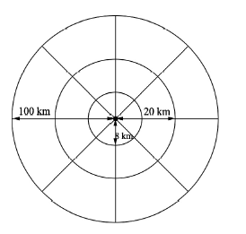
（2）空间匹配：以PM_2.5地面监测点为基准。对AOD而言,以152个监测点经纬度坐标为中心,取其8 km范围内的AOD均值作为Aqua和Terra各自的结果,再对Aqua和Terra的结果取均值,作为该监测点的AOD值。这里需要说明的是之所以取8 km是为了避免经纬度坐标上数据异常、缺失;同时由于卫星扫描时的蝴蝶结效应——随着扫描角度的增大和地球曲率的影响,像素尺寸逐渐增大导致几何变形,数据集像元间所对应的经纬度转换后所得的地理距离会出现大于3 km的情况,因此使用8 km将至少包含目标位置周围的一个像元。对AODs而言,由于气溶胶光学厚度在地理空间上不断传输扩散,某一个位置的空气质量不仅取决于其之前的气溶胶光学厚度,还取决于它邻居的空气质量。为了将空间上分布稀疏的空气质量数据转换为规模一致的大小以便于后续预测模型,按以下策略对AOD进行空间转换处理。如图2所示,以提取监测点气溶胶光学厚度的圆形范围为中心,本文使用和两个同心圆将地理空间划分为16个相邻区域,每个圆圈的半径为20 km和100 km。所有区域都以目标检测站为中心,由内向外区域面积不断扩大。另外不同的角度区域对应不用的地理类型、时间与空间特征。此外,本文对每个区域内所提取到的AOD作汇总平均,每个区域都会有一个平均数值。最后本文可以获得17个AOD,1个来自目标监测点,记为AOD;16个来自相邻区域,记为AODs。本文对每个监测点的时间点都进行上述空间转换处理。

图2

新窗口打开|下载原图ZIP|生成PPT
图2AODs空间转换处理原理图

Fig. 2Schematic diagram of AODs space conversion processing

设计上述转换,主要考虑了以下3个方面。① 考虑到空气污染扩散,由于气溶胶在地理空间上不断扩散,空气质量监测点纪录的空气质量数据可以被视为二手的污染源。利用这些来自空间邻居的信号,后续模型可以获得更多的信息;② 考虑到空间相关性,空间划分将空间分散散乱的气溶胶数据转化为区域级别,较近区域相对较远的区域具有更细的数据空间颗粒度;此外,距离不同的区域对目标的影响与不同的距离有关,这遵循地理学第一定律^[46];③ 考虑的模型可扩展性,空间聚集降低了模型的复杂性,因为它的输入数据有输入上限,即区域数量;而且空间插值可以通过填充缺失值的方式为所有区域生成一致的输入来克服空间稀疏性。这使得本文能够使用不同站点的数据一同用于模型训练,并对深度学习模型做数据增强。

（3）NDVI：以152个监测点经纬度坐标为中心,取其8 km范围内的NDVI均值作为Aqua和Terra各自的结果,再对Aqua和Terra的结果取均值,作为该监测点的NDVI值。需要说明的是,取8 km首先是为了避免由于蝴蝶结效应导致的数据缺失;其次,NDVI数据是16 d产品,如果选定日期内产品数据缺失,对后续时间匹配和缺失值插补造成的影响是严重的,因此扩大提取范围来提高NDVI数据资料的利用率。

（4）气象数据：以152个监测点经纬度坐标为中心,由于气象数据源可调用坐标精细程度与全国城市空气质量实时发布平台公布的监测点经纬度坐标精细程度一致,依照监测点经纬度坐标调用的气象数据可以直接使用。

2.2 基于时空多视图的缺失值插补策略

2.2.1 时空多视图插补策略监测传感器故障导致的数据缺失不仅会影响实时监测数据的连续性和后续数据的可分析性,同时又增加的模型搭建的复杂度,极大干扰了对结果的定性和决策。缺失数据的填补是后续所有相关任务的基础。填补这些带有地理坐标的时间序列数据有以下两个难点：

（1）缺失情况基本是随机的。极端情况下,点的缺失会演变成段状、条状的缺失。当整行、整块缺失时,非负矩阵分解方法难以取得有效的处理结果。

（2）空间上,基于不同类型距离的空间权重矩阵会得到相异插值结果。无论单一使用哪一种距离都会损失其他距离下所蕴含的数据信息。时间上,特征随时间呈周期性变化^{[37,38,39,40,41,42]},而且雨雪恶劣天气会导致时间序列数据的大幅波动,这种特殊变化对后续数据分析起到关键作用,但现有的经典时间序列插值方法会把特殊天气的情况平滑失真。作为常用的纯空间、时间领域的插补方法,虽然能取得较为有效的结果然不可避免地都造成了信息损失,因此需要进一步结合综合了时间与空间的插补方法进行补充,提升信息利用率,降低误差。

为了解决上述难题,本文提出两种插补模块,分别为逐时均值模块以及时空多视图模块,处理日观测数据缺失的数据时,首先尝试使用完整的逐时数据进行插补,取当日24小时的数据均值作为缺失的日观测数据的插补值;如果逐时数据同样缺失,则使用时空多视图插补模块进行插补;最后,使用熵权法融合时空多视图插补模块的结果。

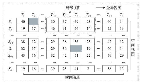
2.2.2 插补算法对每一个特征而言,监测点数据矩阵如下所示,即m个监测点和n个连续时间点。每行均表示一个监测点,每列表示一个时间点。S₁监测点在T₂时间点发生数据缺失,记缺失点为v₁₂;同理可知缺失点v_ji。对于缺失点v₁₂的插补,考虑使用同一时间点的不同相邻监测点的数值插补,如S₁-S₂,本文称之为空间视图;考虑使用同一监测点不同时间点的数值插补例如T₁-T₃,本文称之为时间视图（图3）;其次,对于相邻监测点的相邻范围界定的不同、相邻时间段长度的不同,本文可以获取局部和全局的视图：对部分连续时间点,使用部分相邻的监测点数值来插补,本文称之为局部视图;若是使用所有监测点和时间点的数值来插补则称为全局视图。

图3

新窗口打开|下载原图ZIP|生成PPT
图3多视图插补模块

Fig. 3Multi-view interpolation module

本文对不同插补视图选择合适的插补方法：

① 时间视图使用指数加权平滑插补法（Exponentially Weighted Moving-Average, EWMA）和多项式的插值方法,捕捉时间特性：最终的预测结果是EWMA和多项式插值法的平均预测值。

② 空间视图使用反距离加权插补法（Inverse Distance Weighted, IDW）,捕捉空间特性：IDW根据每个监测点到目标监测点之间的距离来寻找空间相邻监测点,进而根据距离给每个相邻监测点的观测数据分配权重,最后通过对每个空间相邻监测点的观测数据和对应的权重做加权平均。

③ 局部视图使用最近邻估值法（K-Nearest Neighbor, KNN）,捕捉时空交互的邻近相关性：当某一数据缺失,选取空间上相邻（本文取100 km内）的监测点同一特征,同时选取时间上相邻的30个时间点观测数据。计算相邻监测点该30个时间点的观测数据与缺失值时间点观测数据的均方误差,并基于相邻监测点均方误差和的倒数来为这30个时间点分配权重,对目标监测点30个时间点的数据做加权平均。

④ 全局视图使用迭代插补法（Iterative）,捕捉时空交互的长期规律性：进行某一特征插补时,将目标监测点的特征作为被解释特征,其余151个监测点的同一特征作为解释特征,不同时间点相当于不同的样本,进行迭代回归。151个监测点中越是与目标监测点相似性越高,则权重越大。

将以上4种方法的结果分别记为v₁、v₂、v₃、v₄,完成所有数据的时空多视图插补后,将4种视图所在的完整数据使用熵权法获取各自视图的权重,记为w₁、w₂、w₃、w₄,则每个缺失值对应的最终插补结果

\overset{?}{v}

：

（1）

\overset{?}{v} = w_{1} \times v_{1} + w_{2} \times v_{2} + w_{3} \times v_{3} + w_{4} \times v_{4}

2.2.3 插补算法效果检验与结果插补算法的效果从精度和广度两个方面进行验证,结果见表2、表3。

Tab. 2
表2
表2多视图与单视图插补精度检验
Tab. 2Interpolation accuracy tests of multi-view and single-view interpolation

评价标准	多视图		时间视图		空间视图		局部视图		全局视图
评价标准	RE(%)	MAE(μg/m³)	RE(%)	MAE(μg/m³)	RE(%)	MAE(μg/m³)	RE(%)	MAE(μg/m³)	RE(%)	MAE(μg/m³)
PM_2.5	21.3	7.3	68.0	24.7	19.1	6.8	17.8	5.9	16.2	5.2
AOD	24.6	113.4	76.8	283.9	12.3	60.2	20.9	110.6	22.6	76.2
AODs	52.7	136.6	104.5	357.2	50.6	116.7	33.7	116.4	87.6	151.2
NDVI	26.4	0.05	49.8	0.12	12.9	0.02	20.0	0.03	12.3	0.02
气象	12.5	\	36.3	\	15.5	\	15.5	\	21.8	\
平均结果	27.5	\	67.8	\	22.1	\	21.5	\	32.1	\

新窗口打开|下载CSV

Tab. 3
表3
表3多视图与单视图的插补广度比较(%)
Tab. 3The degrees of interpolation completion of multi-view and single-view interpolation (%)

插补方法	插补前	多视图	时间视图	空间视图	局部视图	全局视图
AOD缺失	71.7	0.0	0.4	1.5	2.8	0.0
AODs平均缺失	66.3	0.0	2.9	21.6	42.1	0.0
NDVI缺失	58.6	1.0	24.3	52.2	55.5	34.4
气象数据平均缺失	48.3	22.7	27.3	29.2	37.5	29.4
PM_2.5缺失	15.9	0.5	10.5	3.8	15.5	10.5
平均结果	52.1	4.84	13.1	21.7	30.7	14.9

新窗口打开|下载CSV

① 精度：对每个监测点的每个特征,均随机抽取出25%的非空观测数据并抹去对应位置的观测数据,生成缺失数据。然后,对被抹去位置的缺失数据进行插补,进行20次重复实验,将插补结果与抽取出25%的观测数据进行比较,操作时不统计无法生成插补结果的情况。评价指标使用相对误差（Relative Error, RE）和平均绝对误差（Mean Absolute Error, MAE）。

（2）

\begin{array}{l} RE = \frac{1}{20} \overset{20}{\sum_{j = 1}} \frac{1}{n} \overset{n}{\sum_{i = 1}} |\frac{{\overset{?}{y}}_{ji} - y_{ji}}{y_{ji}}| \\ MAE = \frac{1}{20} \overset{20}{\sum_{j = 1}} \frac{1}{n} \overset{n}{\sum_{i = 1}} |{\overset{?}{y}}_{ji} - y_{ji}| \end{array}

② 广度：使用各视图进行插补,生成2018年度建模数据,并统计各视图插补前后的缺失情况。从表2预测精度,除气象特征外单独使用局部、全局视图时能获得更高的预测精度,其中局部视图的适应性更强,适用于不同的特征领域。尽管时间视图的误差略高,但由于局部视图对块状的数据缺失无法有效插补,空间视图和全局视图对条状缺失无法有效插补,预测误差增大,甚至无法产生插补结果,因此本文在多视图中仍保留时间视图,进而提高插补广度;表2、表3的结果证实将4种视图加权组合的多视图插补能够有效提高插补的精度和广度。最终,获得有效数据42660条,占无缺失情况下样本量的76.9%。

2.3 DP-DNN

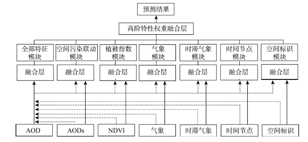
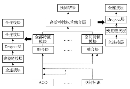
2.3.1 DP-DNN模型架构主要特征和辅助特征会对未来空气质量带来不同的影响,在绝大多数时候,所有的辅助特征将同时决定主要特征的发展环境空间。其次,每一种辅助特征会单独的作用于主要特征来进而影响未来空气质量。同时考虑到特征的滞后作用、不同领域特征间相关性与偏相关性的不一致性,常规的深度神经网络模型难以有效预测PM_2.5浓度值。为了捕捉单独和整体的影响（统称为高阶特性）,DP-DNN架构包含7个神经网络模块,使得主要特征以并行方式来融合每一个辅助特征来捕捉高阶特性,通过将输出线性融合得到最终结果。这样区别特征的原因是主要特征和预测目标来自同一个领域,而辅助特征和预测目标来自于不同的领域。DP-DNN强调了主要特征并捕捉了每一种辅助特征对主要特征的影响从而学习到各种特征之间的高阶特性。

本文指定AOD作为主要输入特征,指定AODs、NDVI、气象,时滞、时间节点和空间标识作为辅助输入特征,7个模块分别为：

（1）空间污染联动模块：用于捕捉污染的空间扩散性和空间相关性。将AOD和AODs一同输入到模块后,可以得到空间污染联动模块。

（2）植被指数模块：用于捕捉植物的背景影响,如土壤、植被覆盖等。既可以反应光照辐射强度、植物生长状态,同时又可以作为监测点所处地理环境结构的特征。

（3）时滞气象模块,气象模块：用于捕捉历史和当日的气象条件对直接特征的影响。本文建立两个模块的原因是由于历史天气数据和当日数据由于本文认为历史和当日数据带来的影响是有区别且复杂的,且前一日的天气条件会影响隔日的天气状况。对于历史和当日气象条件数据,本文将天气、风速、风向、湿度和气压等视为特征。将历史和当日天气状况分别与AOD一同输入到模块后,就可以得到两个模块,即气象模块和时滞气象模块。

（4）时间节点模块,空间标识模块：用来模拟时间和空间地形等特征对空气质量的影响。具体而言,使用时间特征（当前月份）来模拟时间维度上的空气质量规律,例如,由于取暖,冬季总是比夏季具有更高的AOD和PM_2.5浓度。此外,本文使用站点经纬度来模拟地形和空气质量的影响,例如人工聚集区、商业区的空气质量一般来说比公园、林地差。通过将气溶胶数据和时间和空间标识分别融合后,可以得到时间节点模块和空间标识模块。

（5）全部特征融合模块：除单独影响外,所有的间接特征都会同时作用于直接特征,进而影响空气质量的发展环境。为了捕捉这种整体性的影响,本文设计了一个全部特征融合模块,将所有直接和间接特征一同输入到模块后。

最后,本文通过拼接层将捕捉到的七个高阶特性进行连接,采用基于LeakyReLU激活函数进行加权合并,进而模拟这些动态的影响,并产生最终预测。模型流程如图4所示：

图4

新窗口打开|下载原图ZIP|生成PPT
图4DP-DNN架构简易流程图

Fig. 4Flow diagram of DP-DNN algorithm

2.3.2 DP-DNN模块算法架构由于每次融合的输入是大于两个的,无法进行点乘和加法等操作,所以DP-DNN通过使用一个拼接层将输入的特征合并在一起,从而融合所有不同特征。然后使用多个全连接层以非线性的方式学习特征间的高阶特性。为了更好的训练神经网络,在全连接层之间添加一些残差全连接层。残差全连接层通过连接全连接层和残差,可以方便地将前面的信息通过一种跳跃式传递方式传递到后面的网络中,能够有效解决梯度消失、网络退化等问题。在模块中添加一个Dropout层来防止模型过拟合。模块算法架构如图5所示。

图5

新窗口打开|下载原图ZIP|生成PPT
图5DP-DNN模块架构

Fig. 5Module architecture of DP-DNN

2.3.3 特征转换与标准化对分类特征、字符串特征进行特征工程处理,最大限度地从原始数据中提取特征以供算法和模型使用,以便捕捉特征间依赖关系、学习每个影响特征的内部动态。特征工程能够分类特征、字符串特征转换为实数值的向量,并捕捉不同类别之间的相似性。本文将时间节点特征和空间标识特征分别进行特征工程处理,在DP-DNN中捕捉与AOD的相互作用。

数据进行特征融合学习之前,首先对原始数值数据进行标准化^[47]。本文用把输入特征的分布调整到均值为0方差为1的标准正态分布的方法对输入特征进行标准化处理,能够增强输入特征的稳健性,避免梯度消失问题,加快训练速度。

2.3.4 DP-DNN模型参数设置合适的层数和神经元个数是DP-DNN具有优秀性能的基础。经过调优,对于每一个模块,首先从一个大小为24的全连接层开始,连接一个小为24的残差连接层,再添加一个大小分别为12的全连接层和一个rate = 0.01的Dropout层,最后添加两个大小分别为8、4的全连接层;对于高阶特性融合层,是由一个大小为8的全连接层与残差连接层、一个rate = 0.01的Dropout层,一个大小为4的全连接层组成,最后经由激活函数LeakyReLU输出结果;全连接层使用的激活函数均为LeakyReLU;为防止模型过拟合,使用权重为0.01的L2正则化标准;模型编译的优化函数使用学习率为0.01的Adam函数,批量大小为5120,epochs设置为20。

3 结果分析

本文使用2018京津冀鲁4个地区152个监测点的有效数据作为实验数据,借助最小化预测值和地面值之间的平均绝对误差的反向传播训练方法来训练DP-DNN。为了验证预测精度,对样本进行100次随机划分,使用误差均值进行模型评估。其中为了检验模型的时间预测和空间迁移的能力,按如下方法划分训练集和测试集：

（1）时间预测：使用所有监测点的数据,按月份进行对数据随机划分,使得训练集和测试集的样本比值3∶1;

（2）地域迁移：使用2018全年数据,其中对152个监测点进行随机抽样,使得训练集和测试集的样本比值3∶1;

（3）评估指标：使用100次实验的平均绝对误差MAE、相对误差RE,均方误差MSE、均方根误差RMSE的均值来评估模型的仿真结果：

（3）

\begin{array}{l} RE = \frac{1}{100} \overset{100}{\sum_{j = 1}} \frac{1}{n} \overset{n}{\sum_{i = 1}} |\frac{{\overset{?}{y}}_{ji} - y_{ji}}{y_{ji}}| \\ MAE = \frac{1}{100} \overset{100}{\sum_{j = 1}} \frac{1}{n} \overset{n}{\sum_{i = 1}} |{\overset{?}{y}}_{ji} - y_{ji}| \\ MSE = \frac{1}{100} \overset{100}{\sum_{j = 1}} \frac{1}{n} \overset{n}{\sum_{i = 1}} ({\overset{?}{y}}_{ji} - y_{ji})^{2} \\ RMSE = \frac{1}{100} \overset{100}{\sum_{j = 1}} \sqrt[]{\frac{1}{n} \overset{n}{\sum_{i = 1}} ({\overset{?}{y}}_{ji} - y_{ji})^{2}} \end{array}

式中：

y_{ji}

是第j次实验验证集的第i个样本真实值,

{\overset{?}{y}}_{ji}

是第j次实验验证集的第i个样本预测值,n是验证集样本容量。为更直观的对比模型,选用常用模型和本文所运用的模型进行比较。表4为地域迁移检验和时间预测检验的时间开销统计表,图6、图7分别为地域迁移检验和时间预测检验的误差折线图。

Tab. 4
表4
表42018年京津冀鲁地区PM_2.5预测的误差和时间开销
Tab. 4Error and time cost of PM_2.5 concentration prediction based on the Beijing-Tianjin-Hebei-Shandong region in 2018

		DP-DNN			LSTM	GWR	B-OLSR	EN
		地域迁移检验
MAE	16.6		17.2	18.5	22.1	29.1	19.2	21.3
MAE_std	1.1		1.2	1.6	0.9	41.0	0.4	0.6
RE(%)	41.80		44.7	44.6	76.1	141.1	56.6	67.0
RE_std(%)	4.90		4.72	5.0	13.7	141.7	4.3	5.7
MSE	691.5		744.2	901.2	1026.6	63086.4	788.6	1008.9
MSE_std	100.4		103.7	181.1	176.1	275336.9	49.0	81.0
RMSE	26.6		27.2	29.9	31.9	100.3	28.1	31.7
RMSE_std	1.9		1.9	2.9	2.6	230.3	0.9	1.3
		时间预测检验
MAE	17.7		18.9	22.4	25.7	33.7	53.8	21.9
MAE_std	3.7		5.0	7.4	4.7	2.7	12.0	4.3
RE(%)	46.8		50.9	61.9	87.4	108.3	211.2	70.7
RE_std(%)	7.2		11.7	20.8	18.8	26.9	71.3	10.9
MSE	766.2		837.4	1126.8	1645.7	2228.3	3966.7	1038
MSE_std	355.6		446.7	789.5	712.1	532.6	1300	489.7
RMSE	26.9		27.4	31.9	39.6	46.9	62.1	31.3
RMSE_std	6.1		5.0	10.3	8.9	5.1	10.5	7.6
平均耗时(s)	4.2		3.1	3.3	26.4	3389.0	1.3	0.5

新窗口打开|下载CSV

图6

新窗口打开|下载原图ZIP|生成PPT
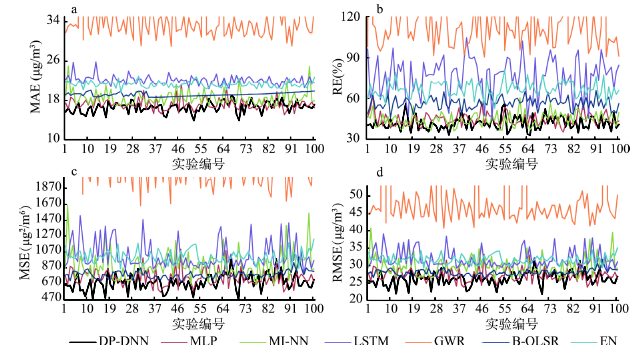
图62018年京津冀鲁地区PM_2.5浓度地域迁移预测的误差折线图

Fig. 6Error line charts of PM_2.5 concentration regional migratory prediction based on the Beijing-Tianjin-Hebei-Shandong region in 2018

图7

新窗口打开|下载原图ZIP|生成PPT
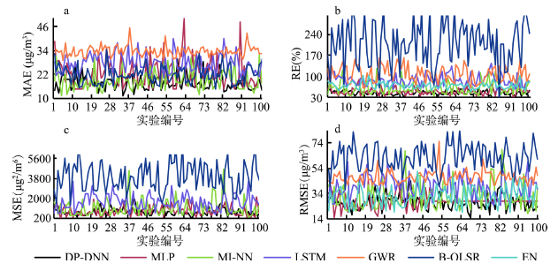
图72018年京津冀鲁地区PM_2.5浓度时间预测检验的误差折线图

Fig. 7Error line charts of PM_2.5 concentration time prediction based on the Beijing-Tianjin-Hebei-Shandong region in 2018

（1）多层神经网络（Multilayer Perceptron, MLP）：仿照DP-DNN“全部特征模块”,模型细节参照DP-NN进行相同设置。引入模型,通过误差对比,验证DP-DNN多模块架构的必要性。

（2）多输入神经网络模型（Multiple Input Neural Network, MI-NN）：仿照DP-DNN,但不区分主要特征和辅助特征。每个模块捕捉每类特征的单独特性,而不是与AOD的交互特性。最后经由激活函数LeakyReLU输出结果,其他模型细节参照DP-NN进行相同设置。

（3）长短期记忆网络模型（Long Short-term Memory, LSTM）：由循环神经网络（RNN）模型改进而来,是一种特殊的递归神经网络,它使用门控机制来捕捉长期依赖性。由于LSTM对数据完整性要求严格,这里输入的特征是PM_2.5浓度、AOD、AODs、时间节点和空间标识。

（4）地理加权模型（Geographically Weighted Regression, GWR）：采用结合了最优带宽自动搜寻的地理加权模型。GWR较多处理输入特征时,在最优带宽的选择上和模型拟合上会产生巨大的时间开销,因此使用的特征是AOD、时间节点和空间标识。

（5）线性回归模型（Boosting Orthogonal Least Squares Regression, B-OLSR）：采用结合了Boosting的最小二乘线性回归模型^[48]。鉴于其难以处理大量离散特征的原因,在使用该模型时将监测点按所属省份进行划分归类;将月份按季度划分归类进行降维。

（6）弹性网络模型（Elastic Network, EN）：由套索模型和岭回归模型改进而来,是一种不断叠代的回归分析方法。

B-OLSR模型难以处理离散特征较多的稀疏矩阵,虽然在随机监测点实验下的预测稳定性较好但是在时间预测检验下误差波动幅度较大;EN通过惩罚项可以有效处理维数的膨胀问题,但预测精度较差;GWR泛化能力低于神经网络模型且在地域迁移预测中误差波动显著增大;从GWR计算速度来看,对于大容量样本计算过程冗杂,在寻找最优带宽和模型拟合过程中耗时格外长;LSTM从多次实验的误差结果来看,模型稳定性很强,但相对DP-DNN而言,误差较大且模型耗时过长;尽管MI-NN、MLP模型速度上小幅领先DP-DNN,但从MAE、RE、MSE、RMSE来看,准确率均低于DP-DNN,且从图表来看,DP-DNN也具有良好的稳定性和短期预测能力,同时也证明了DP-DNN模型的确能够通过多模块的结构捕捉更多的数据信息。

DP-DNN能够有效处理高维特征、捕捉特征间的复杂关系,在处理复杂大气环境污染的研究中表现出了良好的通用性和鲁棒性。与基准模型相比,DP-DNN具有更精细特征粒度、更高阶的特征特性、更合理的网络架构、更快的更新频率,DP-DNN具有优秀的短期时空的迁移预测精度和稳定性,良好的计算速度满足现实应用的需要。DP-DNN是实现历史污染物数据补全,未来污染物浓度、无监测点地区污染物浓度预测的有效手段。

4 结论与展望

本文针对PM_2.5浓度历史数据缺失、监测点覆盖范围小等问题融合了NASA气溶胶光学厚度等多源数据,对缺失值构建并使用时空多视图的插补模型进行插补,弥补了单一插补方法造成的信息损失,其中AOD、AODs完成了全部缺失值的插补。最后,建立的DP-DNN提高了数据利用率和PM_2.5浓度预测精度,在计算速度优越的同时模型短期预测结果更加稳定。构建的DP-DNN模型能够根据给定经纬度,返回3 km×3 km高空间分辨率的PM_2.5浓度预测值,具有很好的应用前景。

基于本文方法估算PM_2.5浓度数据可进一步应用于医学、公共卫生学、经济学和社会学等领域。例如,估算待研究对象居住地点所在栅格的历史长期PM_2.5浓度时间序列数据,结合待研究特定疾病的发病率、死亡率和门诊率等健康效应指标进行慢性健康效应研究,为PM_2.5长期暴露与疾病的因果关系研究增加证据;估算省域历史PM_2.5年均浓度,结合统计年鉴数据建立计量模型进行城镇化推进、城市群发展、转变经济发展方式成效等问题的分析。

参考文献原文顺序
文献年度倒序
文中引用次数倒序
被引期刊影响因子

[1]

Geng G

, Zhang

, Martin R

, et al. Estimating long-term PM_2.5 concentrations in China using satellite-based aerosol optical depth and a chemical transport model
Remote Sensing of Environment, 2015,166:262-270.

[本文引用: 1]

[2]

Lee

, Mukhopadhyay

, Rushworth

, et al. A rigorous statistical framework for spatio-temporal pollution prediction and estimation of its long-term impact on health
Biostatistics, 2017,18(2):370-385.

[本文引用: 1]

[3]

Mukhopadhyay

, Sahu S

. A Bayesian spatiotemporal model to estimate long-term exposure to outdoor air pollution at coarser administrative geographies in England and Wales
Journal of the Royal Statistical Society: Series A (Statistics in Society), 2018,181(2):465-486.

[本文引用: 1]

[4]

Fang

, Zou

, Liu

, et al. Satellite-based ground PM_2.5 estimation using timely structure adaptive modeling
Remote Sensing of Environment, 2016,186:152-163.

[本文引用: 2]

[5]

van Donkelaar

, Martin R

, Brauer

, et al. Global estimates of fine particulate matter using a combined geophysical-statistical method with information from satellites, models, and monitors
Environmental Science & Technology, 2016,50(7):3762-3772.

DOI:10.1021/acs.est.5b05833 URLPMID:26953851 [本文引用: 2]

We estimated global fine particulate matter (PM2.5) concentrations using information from satellite-, simulation- and monitor-based sources by applying a Geographically Weighted Regression (GWR) to global geophysically based satellite-derived PM2.5 estimates. Aerosol optical depth from multiple satellite products (MISR, MODIS Dark Target, MODIS and SeaWiFS Deep Blue, and MODIS MAIAC) was combined with simulation (GEOS-Chem) based upon their relative uncertainties as determined using ground-based sun photometer (AERONET) observations for 1998-2014. The GWR predictors included simulated aerosol composition and land use information. The resultant PM2.5 estimates were highly consistent (R(2) = 0.81) with out-of-sample cross-validated PM2.5 concentrations from monitors. The global population-weighted annual average PM2.5 concentrations were 3-fold higher than the 10 mug/m(3) WHO guideline, driven by exposures in Asian and African regions. Estimates in regions with high contributions from mineral dust were associated with higher uncertainty, resulting from both sparse ground-based monitoring, and challenging conditions for retrieval and simulation. This approach demonstrates that the addition of even sparse ground-based measurements to more globally continuous PM2.5 data sources can yield valuable improvements to PM2.5 characterization on a global scale.

[6]

He Q

, Huang

. Satellite-based mapping of daily high-resolution ground PM_2.5 in China via space-time regression modeling
Remote Sensing of Environment, 2018,206:72-83.

[本文引用: 1]

[7]

Wang Z

, Chen L

, Tao J

, et al. Satellite-based estimation of regional particulate matter (PM) in Beijing using vertical-and-RH correcting method
Remote Sensing of Environment, 2010,114(1):50-63.

[本文引用: 1]

[8]

Fu D

, Xia X

, Wang

, et al. Synergy of AERONET and MODIS AOD products in the estimation of PM_2.5 concentrations in Beijing
Scientific Reports, 2018,8(1):10174-10181.

DOI:10.1038/s41598-018-28535-2 URLPMID:29977000 [本文引用: 2]

[9]

Wang

, Christopher S

. Intercomparison between satellite-derived aerosol optical thickness and PM_2.5 mass: Implications for air quality studies
Geophysical Research Letters, 2003,30(21):2095-2098.

[本文引用: 1]

[10]

Engel-Cox J

, Holloman C

, Coutant B

, et al. Qualitative and quantitative evaluation of MODIS satellite sensor data for regional and urban scale air quality
Atmospheric Environment, 2004,38(16):2495-2509.

DOI:10.1016/j.atmosenv.2004.01.039 URL [本文引用: 1]

[11]

Jia

Songlin

, Su

Lin

, Tao

Jinhua

, et al. A study of multiple regression method for estimating concentration of fine particulate matter using satellite remote sensing
China Environmental Science, 2014,34(3):565-573.

[本文引用: 3]

[ 贾松林, 苏林, 陶金花, 等. 卫星遥感监测近地表细颗粒物多元回归方法研究
中国环境科学, 2014,34(3):565-573.]

[本文引用: 3]

[12]

Zang Z

, Wang W

, Cheng X

, et al. Effects of boundary layer height on the model of ground-level PM_2.5 concentrations from AOD: Comparison of stable and convective boundary layer heights from different methods
Atmosphere, 2017,8:104-121.

[本文引用: 3]

[13]

Gupta

, Christopher S

. Particulate matter air quality assessment using integrated surface, satellite, and meteorological products: Multiple regression approach
Journal of Geophysical Research Atmospheres, 2009,114:D14205. DOI: 10.1029/2008JD011497.

[本文引用: 2]

[14]

Koelemeijer R B

, Homan C

, Matthijsen

. Comparison of spatial and temporal variations of aerosol optical thickness and particulate matter over Europe
Atmospheric Environment, 2006,40(27):5304-5315.

[本文引用: 2]

[15]

Chen

Hui

, Li

Qing

, Zhang

Yuhuan

, et al. Estimations of PM_2.5 concentrations based on the method of geographically weighted regression
Acta Scientiae Circumstantiae, 2016,36(6):2142-2151.

[本文引用: 2]

[ 陈辉, 厉青, 张玉环, 等. 基于地理加权模型的我国冬季PM_2.5遥感估算方法研究
环境科学学报, 2016,36(6):2142-2151.]

[本文引用: 2]

[16]

He Q

, Huang

. Satellite-based high-resolution PM_2.5 estimation over the Beijing-Tianjin-Hebei region of China using an improved geographically and temporally weighted regression model
Environmental Pollution, 2018,236:1027-1037.

DOI:10.1016/j.envpol.2018.01.053 URLPMID:29455919 [本文引用: 1]

Ground fine particulate matter (PM2.5) concentrations at high spatial resolution are substantially required for determining the population exposure to PM2.5 over densely populated urban areas. However, most studies for China have generated PM2.5 estimations at a coarse resolution (>/=10km) due to the limitation of satellite aerosol optical depth (AOD) product in spatial resolution. In this study, the 3km AOD data fused using the Moderate Resolution Imaging Spectroradiometer (MODIS) Collection 6 AOD products were employed to estimate the ground PM2.5 concentrations over the Beijing-Tianjin-Hebei (BTH) region of China from January 2013 to December 2015. An improved geographically and temporally weighted regression (iGTWR) model incorporating seasonal characteristics within the data was developed, which achieved comparable performance to the standard GTWR model for the days with paired PM2.5- AOD samples (Cross-validation (CV) R(2)=0.82) and showed better predictive power for the days without PM2.5- AOD pairs (the R(2) increased from 0.24 to 0.46 in CV). Both iGTWR and GTWR (CV R(2)=0.84) significantly outperformed the daily geographically weighted regression model (CV R(2)=0.66). Also, the fused 3km AODs improved data availability and presented more spatial gradients, thereby enhancing model performance compared with the MODIS original 3/10km AOD product. As a result, ground PM2.5 concentrations at higher resolution were well represented, allowing, e.g., short-term pollution events and long-term PM2.5 trend to be identified, which, in turn, indicated that concerns about air pollution in the BTH region are justified despite its decreasing trend from 2013 to 2015.

[17]

Chen

Hui

, Li

Qing

, Wang

Zhongting

, et al. Utilization of MERSI and MODIS data to monitor PM_2.5 concentration in Beijing-Tianjin-Hebei and its surrounding areas
Journal of Remote Sensing, 2018,22(5):822-832.

[本文引用: 1]

[ 陈辉, 厉青, 王中挺, 等. MERSI和MODIS卫星监测京津冀及周边地区PM_2.5浓度
遥感学报, 2018,22(5):822-832.]

[本文引用: 1]

[18]

Jiang

, Sun W

, Yang

, et al. Modelling seasonal GWR of daily PM_2.5 with proper auxiliary variables for the Yangtze River Delta
Remote Sensing, 2017,9(4):346. DOI: 10.3390/rs9040346.

[本文引用: 1]

[19]

Wu J

, Yao

, Li W

, et al. VIIRS-based remote sensing estimation of ground-level PM_2.5 concentrations in Beijing-Tianjin-Hebei: A spatiotemporal statistical model
Remote Sensing of Environment, 2016,184:316-328.

[本文引用: 2]

[20]

Wu Y

, Guo J

, Zhang X

, et al. Synergy of satellite and ground based observations in estimation of particulate matter in eastern China
Science of the Total Environment, 2012,433:20-30.

[本文引用: 1]

[21]

Yao

, Lu

. Spatiotemporal distribution and short-term trends of particulate matter concentration over China, 2006-2010
Environmental Science and Pollution Research, 2014,21(16):9665-9675.

URLPMID:24824505 [本文引用: 1]

[22]

Shao

, Chen

Yunhao

, Li

Jing

. Inversion of PM_2.5 concentration in Beijing based on satellite remote sensing and meteorological reanalysis data
Geography and Geo-Information Science, 2018,34(3):32-38.

[本文引用: 3]

[ 邵琦, 陈云浩, 李京. 基于卫星遥感和气象再分析资料的北京市PM_2.5浓度反演研究
地理与地理信息科学, 2018,34(3):32-38.]

[本文引用: 3]

[23]

Zou

, Chen J

, Zhai

, et al. Satellite based mapping of ground PM_2.5 concentration using generalized additive modeling
Remote Sensing, 2016,9(1):1. DOI: 10.3390/rs9010001.

[本文引用: 1]

[24]

Kloog

, Koutrakis

, Coull B

, et al. Assessing temporally and spatially resolved PM_2.5 exposures for epidemiological studies using satellite aerosol optical depth measurements
Atmospheric Environment, 2011,45(35):6267-6275.

[本文引用: 1]

[25]

Sorek-Hamer

, Strawa A

, Chatfield R

, et al. Improved retrieval of PM_2.5 from satellite data products using non-linear methods
Environmental Pollution, 2013,182:417-423.

DOI:10.1016/j.envpol.2013.08.002 URLPMID:23995022 [本文引用: 1]

Satellite observations may improve the areal coverage of particulate matter (PM) air quality data that nowadays is based on surface measurements. Three statistical methods for retrieving daily PM2.5 concentrations from satellite products (MODIS-AOD, OMI-AAI) over the San Joaquin Valley (CA) are compared--Linear Regression (LR), Generalized Additive Models (GAM), and Multivariate Adaptive Regression Splines (MARS). Simple LRs show poor correlations in the western USA (R(2) ~/= 0.2). Both GAM and MARS were found to perform better than the simple LRs, with a slight advantage to the MARS over the GAM (R(2) = 0.71 and R(2) = 0.61, respectively). Since MARS is also characterized by a better computational efficiency than GAM, it can be used for improving PM2.5 retrievals from satellite aerosol products. Reliable PM2.5 retrievals can fill in missing surface measurements in areas with sparse ground monitoring coverage and be used for evaluating air quality models and as exposure metrics in epidemiological studies.

[26]

Li T

, Shen H

, Zeng

, et al. Point-surface fusion of station measurements and satellite observations for mapping PM_2.5 distribution in China: Methods and assessment
Atmospheric Environment, 2017,152:477-489.

[本文引用: 1]

[27]

Lyu

, Dai

, Zheng Y

, et al. Estimation of PM_2.5 concentrations over Beijing with MODIS AODs using an artificial neural network
Scientific Online Letters on the Atmosphere, 2018,14:14-18.

[28]

Zou

, Wang

, Wan

, et al. Spatial modeling of PM_2.5 concentrations with a multifactoral radial basis function neural network
Environmental Science and Pollution Research, 2015,22(14):10395-10404.

DOI:10.1007/s11356-015-4380-3 URLPMID:25813644

Accurate measurements of PM2.5 concentration over time and space are especially critical for reducing adverse health outcomes. However, sparsely stationary monitoring sites considerably hinder the ability to effectively characterize observed concentrations. Utilizing data on meteorological and land-related factors, this study introduces a radial basis function (RBF) neural network method for estimating PM2.5 concentrations based on sparse observed inputs. The state of Texas in the USA was selected as the study area. Performance of the RBF models was evaluated by statistic indices including mean square error, mean absolute error, mean relative deviation, and the correlation coefficient. Results show that the annual PM2.5 concentrations estimated by the RBF models with meteorological factors and/or land-related factors were markedly closer to the observed concentrations. RBF models with combined meteorological and land-related factors achieved best performance relative to ones with either type of these factors only. It can be concluded that meteorological factors and land-related factors are useful for articulating the variation of PM2.5 concentration in a given study area. With these covariate factors, the RBF neural network can effectively estimate PM2.5 concentrations with acceptable accuracy under the condition of sparse monitoring stations. The improved accuracy of air concentration estimation would greatly benefit epidemiological and environmental studies in characterizing local air pollution and in helping reduce population exposures for areas with limited availability of air quality data.

[29]

Yao

, Lu

, Jiang

. Artificial Neural Network (ANN) for multi-source PM_2.5 estimation using surface, MODIS, and meteorological data
Proceedings of the 2012 International Conference on Biomedical Engineering and Biotechnology, 2012: 1228-1231.

[本文引用: 1]

[30]

Mei

, Tian

Maozai

. Analysis of influential factors on PM_2.5 in Beijing based on spatio-temporal model
Journal of Applied Statistics and Management, 2018,37(4):571-586.

[本文引用: 1]

[ 梅波, 田茂再. 基于时空模型北京市PM_2.5浓度影响因素研究
数理统计与管理, 2018,37(4):571-586.]

[本文引用: 1]

[31]

Ellett F S

, Ericson D

. Correlation, partial correlation, and causation
Synthese, 1986,67(2):157-173.

[本文引用: 1]

[32]

Wang W

, Zhao S

, Jiao L

, et al. Estimation of PM_2.5 concentrations in China using a spatial back propagation neural network
Scientific Reports, 2019,9:13788. DOI: 10.1038/s41598-019-50177-1.

URLPMID:31551510 [本文引用: 1]

Methods for estimating the spatial distribution of PM2.5 concentrations have been developed but have not yet been able to effectively include spatial correlation. We report on the development of a spatial back-propagation neural network (S-BPNN) model designed specifically to make such correlations implicit by incorporating a spatial lag variable (SLV) as a virtual input variable. The S-BPNN fits the nonlinear relationship between ground-based air quality monitoring station measurements of PM2.5, satellite observations of aerosol optical depth, meteorological synoptic conditions data and emissions data that include auxiliary geographical parameters such as land use, normalized difference vegetation index, elevation, and population density. We trained and validated the S-BPNN for both yearly and seasonal mean PM2.5 concentrations. In addition, principal components analysis was employed to reduce the dimensionality of the data and a grid of neural network models was run to optimize the model design. The S-BPNN was cross-validated against an analogous but SLV-free BPNN model using the coefficient of determination (R(2)) and root mean squared error (RMSE) as statistical measures of goodness of fit. The inclusion of the SLV led to demonstrably superior performance of the S-BPNN over the BPNN with R(2) values increasing from 0.80 to 0.89 and with the RMSE decreasing from 8.1 to 5.8 mug/m(3). The yearly mean PM2.5 concentration in China during the study period was found to be 41.8 mug/m(3) and the model estimated spatial distribution was found to exceed Level 2 of the China Ambient Air Quality Standards (CAAQS) enacted in 2012 (>35 mug/m(3)) in more than 70% of the Chinese territory. The inclusion of spatial correlation upgrades the performance of conventional BPNN models and provides a more accurate estimation of PM2.5 concentrations for air quality monitoring.

[33]

Wang X

, Wang

, Jia L

, et al. Retrieval and validation of aerosol optical depth using GF-1 WFV cameras data
Advances in Space Research, 2020,65(3):997-1007.

[本文引用: 1]

[34]

Yu W

, Nan Z

, Wu T

, et al. An effective interpolation method for MODIS land surface temperature on the Qinghai-Tibet Plateau
IEEE Journal of Selected Topics in Applied Earth Observations and Remote Sensing, 2015,8(9):4539-4550.

[本文引用: 1]

[35]

Safarpour

, Abdullah

, Lim H

, et al. Spatial interpolation of aerosol optical depth pollution: Comparison of methods for the development of aerosol distribution. ISPRS: International Archives of the Photogrammetry,
Remote Sensing and Spatial Information Sciences, 2017,4(4):237-244.

[本文引用: 1]

[36]

Sathe

, Kulkarni

, Gupta

, et al. Application of moderate resolution imaging spectroradiometer (MODIS) aerosol optical depth (AOD) and weather research forecasting (WRF) model meteorological data for assessment of fine particulate matter (PM_2.5) over India
Atmospheric Pollution Research, 2019,10(2):418-434.

[本文引用: 1]

[37]

Beckerman B

, Jerrett

, Serre

, et al. A hybrid approach to estimating national scale spatiotemporal variability of PM_2.5 in the contiguous United States
Environmental Science & Technology, 2013,47(13):7233-7241.

DOI:10.1021/es400039u URLPMID:23701364 [本文引用: 2]

Airborne fine particulate matter exhibits spatiotemporal variability at multiple scales, which presents challenges to estimating exposures for health effects assessment. Here we created a model to predict ambient particulate matter less than 2.5 mum in aerodynamic diameter (PM2.5) across the contiguous United States to be applied to health effects modeling. We developed a hybrid approach combining a land use regression model (LUR) selected with a machine learning method, and Bayesian Maximum Entropy (BME) interpolation of the LUR space-time residuals. The PM2.5 data set included 104,172 monthly observations at 1464 monitoring locations with approximately 10% of locations reserved for cross-validation. LUR models were based on remote sensing estimates of PM2.5, land use and traffic indicators. Normalized cross-validated R(2) values for LUR were 0.63 and 0.11 with and without remote sensing, respectively, suggesting remote sensing is a strong predictor of ground-level concentrations. In the models including the BME interpolation of the residuals, cross-validated R(2) were 0.79 for both configurations; the model without remotely sensed data described more fine-scale variation than the model including remote sensing. Our results suggest that our modeling framework can predict ground-level concentrations of PM2.5 at multiple scales over the contiguous U.S.

[38]

Chow J

, Chen

L W A

, Watson

J G

, et al. PM_2.5 chemical composition and spatiotemporal variability during the California Regional PM₁₀/PM_2.5 Air Quality Study (CRPAQS)
Journal of Geophysical Research: Atmospheres, 2006,111(10). DOI: 10.1029/2005jd006457.

[本文引用: 2]

[39]

Lin

, Fu

, Jiang

, et al. Spatio-temporal variation of PM_2.5 concentrations and their relationship with geographic and socioeconomic factors in China
International Journal of Environmental Research and Public Health, 2013,11(1):173-186.

URLPMID:24362546 [本文引用: 2]

[40]

Gelencsér

, May

, Simpson

, et al. Source apportionment of PM_2.5 organic aerosol over Europe: Primary/secondary, natural/anthropogenic, and fossil/biogenic origin
Journal of Geophysical Research: Atmospheres, 2007, 112:17D23S043. DOI: 10.1029/2006JD008094.

[本文引用: 2]

[41]

Liu

, Paciorek C

, Koutrakis

. Estimating regional spatial and temporal variability of PM_2.5 Concentrations using satellite data, meteorology, and land use information
Environmental Health Perspectives, 2009,117(6):886-892.

DOI:10.1289/ehp.0800123 URLPMID:19590678 [本文引用: 2]

[42]

Kloog

, Nordio

, Coull B

, et al. Incorporating local land use regression and satellite aerosol optical depth in a hybrid model of spatiotemporal PM_2.5 exposures in the Mid-Atlantic states
Environmental Science & Technology, 2012,46(21):11913-11921.

DOI:10.1021/es302673e URLPMID:23013112 [本文引用: 2]

Satellite-derived aerosol optical depth (AOD) measurements have the potential to provide spatiotemporally resolved predictions of both long and short-term exposures, but previous studies have generally shown moderate predictive power and lacked detailed high spatio- temporal resolution predictions across large domains. We aimed at extending our previous work by validating our model in another region with different geographical and metrological characteristics, and incorporating fine scale land use regression and nonrandom missingness to better predict PM(2.5) concentrations for days with or without satellite AOD measures. We start by calibrating AOD data for 2000-2008 across the Mid-Atlantic. We used mixed models regressing PM(2.5) measurements against day-specific random intercepts, and fixed and random AOD and temperature slopes. We used inverse probability weighting to account for nonrandom missingness of AOD, nested regions within days to capture spatial variation in the daily calibration, and introduced a penalization method that reduces the dimensionality of the large number of spatial and temporal predictors without selecting different predictors in different locations. We then take advantage of the association between grid-cell specific AOD values and PM(2.5) monitoring data, together with associations between AOD values in neighboring grid cells to develop grid cell predictions when AOD is missing. Finally to get local predictions (at the resolution of 50 m), we regressed the residuals from the predictions for each monitor from these previous steps against the local land use variables specific for each monitor.

[43]

National Oceanic and Atmospheric Administration Weather Prediction Center. The Heat Index Equation[EB/OL]. (2014-05-28) [2019-08-13]. http://www.wpc.ncep.noaa.gov/html/heatindex_equation.shtml.

URL [本文引用: 1]

[44]

National Aeronautics and Space Administration. MODIS Standard Collection 6.1 Update Executive Summary[EB/OL]. (2017-08-09) [2019-08-20]. https://atmosphere-imager.gsfc.nasa.gov/documentation/collection-61.

URL [本文引用: 1]

[45]

Dark Sky Docs: Data Sources[EB/OL]. (2019-09-04) [2019-08-24]. https://darksky.net/dev/docs/sources.

URL [本文引用: 1]

[46]

Tobler W

. A computer movie simulating urban growth in the Detroit Region
Economic Geography, 1970,46:234-240.

[本文引用: 1]

[47]

Swami

, Jain

. Scikit-learn: Machine learning in Python
Journal of Machine Learning Research, 2013,12(10):2825-2830.

[本文引用: 1]

[48]

Wang X

, Brown D

. Boosting orthogonal least squares regression
Lecture Notes in Computer Science, 2004,3177:678-683.

[本文引用: 1]