HTML
--> --> -->A multinational joint ?eld campaign called the Dynamics of MJO/Cooperative Indian Ocean Experiment on Intraseasonal Variability in the Year 2011 (DYNAMO/CINDY 2011) took place over the equatorial Indian Ocean from late 2011 to early 2012 to further understand the key physical processes related to the MJO (Yoneyama et al., 2013). Based on the in-situ observations, numerous studies have revealed the importance of low-level moisture and circulation in triggering the MJO convection. Gottschalck et al. (2013) indicated that the enhanced convective phases of MJO events have a close relationship with the activities of equatorial Rossby waves. Moum et al. (2014) documented intense multi-scale interactions within the MJO convection envelope. Oh et al. (2015) found that the lower-level westerly acceleration induced by the pressure gradient force accounts for the establishment of a baroclinic wind structure following the MJO convection.
Different theories and mechanisms have been proposed to explain the MJO from various aspects, as summarized in Li (2014), Wang et al. (2016), Jiang et al. (2020), and Zhang et al. (2020). Numerous studies have shown that the MJO exhibits a distinctive multi-scale structure (Nakazawa, 1988; Mapes et al., 2006; Moncrieff et al., 2012). Some mechanisms have been proposed to explain how the mesoscale and synoptic-scale motions interact with the MJO and how they contribute to the MJO dynamics. For example, the MJO skeleton model (Majda and Biello, 2004; Biello and Majda, 2005; Majda and Stechmann, 2009) considers the upscale momentum, heat, and moisture transports from synoptic-scale systems as potential drivers for the MJO. They noted the westerly and easterly regimes of flows and wave trains of tilted organized synoptic-scale circulations are important in modeling the multi-scale for the MJO. The MJO-synoptic wave interaction model also confirms the upscale momentum transfer of superclusters can drive the MJO-like circulation (Wang and Liu, 2011; Liu et al., 2012; Liu and Wang, 2013). This MJO-synoptic wave interaction model allows for two-way interaction between the high-frequency waves (inertial-gravity waves, Kelvin waves) and the MJO. It indicates that the relative location of the synoptic disturbance to the MJO convection center is essential for the MJO. These theories have significantly advanced our understanding of the MJO. However, the influence of the MJO multi-scale structure on the development and evolution of the MJO convection still needs to be further explored.
The budget diagnostic for moisture (Sobel et al., 2014; Mei et al., 2015), temperature (Zhao et al., 2013), and kinetic energy (Zhou et al., 2012; Krishnamurti et al., 2016) have been used to reveal the actual physical processes related to the MJO. Energy diagnosis is one of the most important ways to understand the physical processes in the atmosphere. One advantage of the kinetic energy budget analysis is that it can reveal the energy transformation among different physical processes and the interaction between different scales. Several energy diagnostic methods have been proposed to explore the multi-scale interactions of MJO. Hsu et al. (2011, 2017) used the eddy kinetic energy budget analysis to investigate interactions between synoptic-scale disturbances and the MJO. This eddy energy diagnostic method separates the effects of the MJO and low-frequency background state on the eddy, which provides a way to explore the interaction between different scales. Similarly, the mean kinetic energy budget analysis has been applied to study the interaction between the mean flow and intraseasonal oscillation (Hsu and Yang, 2016). Both methods mentioned above illustrate the interaction between the MJO and synoptic-scale systems/mean flow to a certain extent, but neither can directly obtain the two-way interaction process between MJO and synoptic-scale systems/mean flow. Zhou et al. (2012) explored the evolution of the MJO kinetic energy by decomposing all variables into three components based on the spatial scale: the zonal mean, the MJO scale, and the small scale. This method provides a better way to explore the related physical process that causes the kinetic energy change of the MJO. But it cannot offer the two-way scale interaction between the MJO and synoptic-scale disturbances. Krishnamurti et al. (2016) used the Lorenz box energetics on synoptic scales to analyze the effect of synoptic-scale systems on the MJO during the active phase of the MJO. Their results show that the convection is only organized at the scale of synoptic/mesoscale disturbances but not at the space and time scales of the MJO. The results suggest that the MJO convection is maintained by the synoptic scale systems via nonlinear energy transfers. Hsu et al. (2018) obtained the kinetic energy equation at the MJO scale by filtering the momentum equation. Their results show the low-level MJO gains KE from the background mean flow during central Pacific El Ni?o events but loses KE to high-frequency eddies. The advection terms that enable interactions between different scales in the momentum equation are nonlinear. Thus the direct filtering of advection terms may cause incompleteness of nonlinear multi-scale interaction terms. All the methods mentioned above helped to advance our understanding of the interactions between MJO and other scales. However, some of them focused on kinetic energy sources of other time scale variabilities rather than the MJO, and some cannot fully explore the local interaction between MJO and other time scale variabilities.
By introducing the local interaction energy and its flux, Murakami (2011) reconstructed the classical energetics analysis and provided a diagnostic tool for the local energy analysis. This method divides the basic variables into time-mean and transient-eddy components and provides each component with corresponding energy equations. It is challenging to describe the local features of the Lorenz energy cycle. For a local energy cycle, the energy conversion term from mean flow to eddy in the energy equations derived for mean flow is different from that derived in the kinetic energy equation for the eddy. Therefore, it is difficult to interpret which expression should be used for the local energy conversion (Holopainen, 1978). Unlike a global view of the energy cycle, the local energy framework introduces the concept of interaction energy. Thus, it provides a feasible way to interpret the local features of the energy conversion between the mean and eddy fields (Murakami, 2011). The local energy framework also gives complete information about the three-dimensional structure of the energy interactions between different time scales. Given the advantages of the local energetics framework, we aim to construct a new kinetic energy budget method following Murakami (2011) that allows us to investigate the local kinetic energy budget and the multi-scale interaction of the MJO. Unlike Murakami (2011), the basic variables are decomposed into three components: high-frequency, MJO, and low-frequency background state (LFBS). In this study, we attempt to reveal the kinetic energy transport and conversion processes of MJO, high-frequency disturbances, and LFBS when the MJO convection propagates over the Indian Ocean at its rapidly developing stage. Applying this kinetic energy budget for an MJO case can shed light on understanding the energy transport path of MJO and lays the foundation for analyzing the common energy budget features of all the MJO events.
The remaining part of this paper is organized as follows. Section 2 describes the data and the derivation of the kinetic energy diagnostic equations. Section 3 introduces the general information of the DYNAMO MJO cases. Section 4 provides the detailed results for each term in the MJO and high-frequency kinetic energy diagnostic scheme as well as the interaction between MJO and high-frequency disturbances. Summary and discussions are given in section 5.
2.1. Data
Daily three-dimensional wind fields (u, v, ω), temperature (T), and geopotential (Φ) from the European Centre for Medium-Range Weather Forecasts (ECMWF) Interim reanalysis (ERA-Interim; Dee et al., 2011) were used for the energy budget analysis. The horizontal resolution is 0.75° × 0.75°, and vertical resolutions are 25 hPa for 1000?750 hPa, 50 hPa for 750?250 hPa, and 25 hPa for 250?100 hPa. The daily satellite-observed outgoing longwave radiation (OLR) data with a horizontal resolution of 2.5° × 2.5° from the NOAA/Earth System Research Laboratory (ESRL; Liebmann and Smith, 1996) was used to represent the deep convection. The rainfall dataset from the Tropical Rainfall Measuring Mission (TRMM) Multi-satellite Precipitation Analysis, version 7 (Huffman et al., 2007) with a horizontal resolution of 0.25° × 0.25° was used for the large-scale overview of precipitation. All the datasets mentioned above cover the period from 1 January 2011 to 31 December 2012 in this study.2
2.2. Method
A multi-scale interaction energy diagnostic scheme for the local atmospheric energy is derived in this study. It is impractical to construct an utterly closed energy budget system based on reanalysis datasets because of the lack of certain variables, such as friction, convective heating, and other variables related to unresolved sub-grid processes. Thus, only the terms which can be derived from the reanalysis datasets are discussed here. We start from a set of primitive equations in isobaric coordinates:where t is time, p is pressure, u, v, and ω are the three-dimensional wind speeds, Ф is the geopotential, f is the Coriolis parameter, α = RT/p is speci?c volume, with T and R being the temperature and gas constant, respectively, Fx and Fy are residuals denoting all unresolved processes (e.g., friction force and sub-grid processes).
Different from Murakami (2011), all variables are decomposed into three components: the LFBS (period longer than 100 days), the MJO (20?100-day), and the high-frequency (period shorter than 20 days) components. For a given variable X, it could be decomposed into the following three terms:
where


Furthermore, those components also satisfied the following assumptions:


In this case, the kinetic energy (KE) K is divided into six terms as
where


Before obtaining the KE equation of the MJO, the equations of motion for each scale are firstly obtained. For example, the zonal momentum equation of LFBS is obtained by applying 100-day running mean for Eq. (1a),
where


Finally, the zonal momentum equation at the MJO scale can be obtained by subtracting Eq. (4) and Eq. (5) from Eq. (1a),
Similarly, Eq. (1b) to Eq. (1d) can also be decomposed into different time scales. By applying the inner product with

Eq. (7a) is the MJO KE budget equation. The symbol


Similarly, by applying the inner product with

Eq. (8a) is the budget equation for the high-frequency KE. The right-handed terms have a similar physical meaning as Eqs. (7b?f) but for the high-frequency KE.
There is another term related to the MJO energy in the KE budget equations of LFBS, the KE conversion from


The interaction energy flux is an important concept in this diagnostic scheme. Taking the interaction between MJO and high-frequency disturbances as an example, when averaging over the entire global atmosphere, the energy conversion terms,


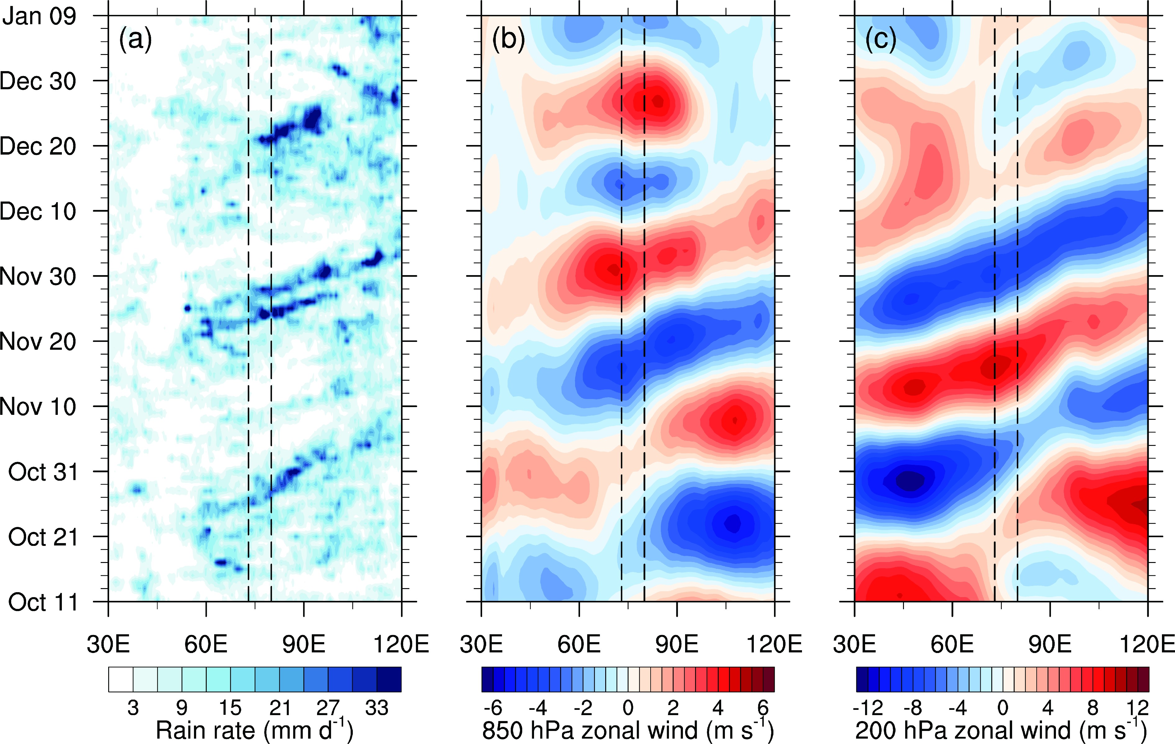 Figure1. Hovm?ller diagrams of (a) TRMM precipitation (units: mm d?1), 20-100-day filtered (b) 850 hPa and (c) 200 hPa zonal wind anomalies (units: m s?1) averaged between 10°S?10°N from 1 October 2011 to 14 January 2012. Dashed black lines mark the west and east boundaries of the sounding arrays (73°?80°E) for the DYNAMO field campaign.
The horizontal distributions of rainfall and wind fields in MJO I and MJO II are obviously different (Johnson and Ciesielski, 2013). The wind over the Indian Ocean is weaker during the evolution of MJO I than that of MJO II. The main body of MJO I convection is inclined to the north of the equator, and the precipitation is relatively weak (Johnson and Ciesielski, 2013; Oh et al., 2015). This is consistent with the lower tropospheric MJO KE evolution of MJO I. The precipitation is almost evenly distributed on both sides of the equator, and it has a swallowtail pattern during the MJO II convection active phase (Fig. 2b), which is more consistent with the typical horizontal distribution of the MJO convection (Zhang and Ling, 2012; Adames and Wallace, 2014). Therefore, the kinetic budget analysis was applied to MJO II when its convection is active over the tropical Indian Ocean (10°S?10°N, 60°?90°E).
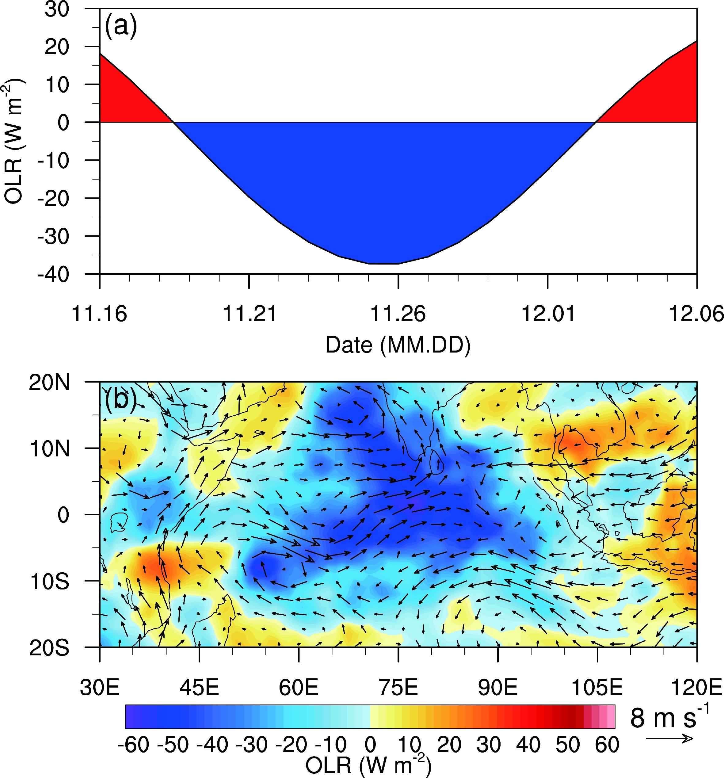 Figure2. (a) Time series of 20-100-day filtered OLR anomalies (units: W m?2) averaged over the tropical Indian Ocean (10°S?10°N, 60°?90°E); (b) horizontal distributions of 20-100-day filtered anomalous OLR (color; units: W m?2) and horizontal wind at 850 hPa (vector; units: m s?1) on 26 November 2011.
The strengthening and weakening stages of the MJO II are determined based on the time evolution of the observed intraseasonal (20?100-day filtered) OLR anomalies averaged over the tropical Indian Ocean (Fig. 2a). The intraseasonal OLR anomalies transitioned from positive to negative phase on 19 November, reached their minimum on 26 November, and returned to positive on 2 December for MJO II. Therefore, the strengthening stage of MJO II is from 19 November to 26 November, and its weakening stage is from 27 November to 2 December.
4.1. Kinetic energy analysis
To understand the evolution of the MJO KE structure and its relationship with the MJO convection, the time-longitude evolution of the mass-weighted mean MJO KE (

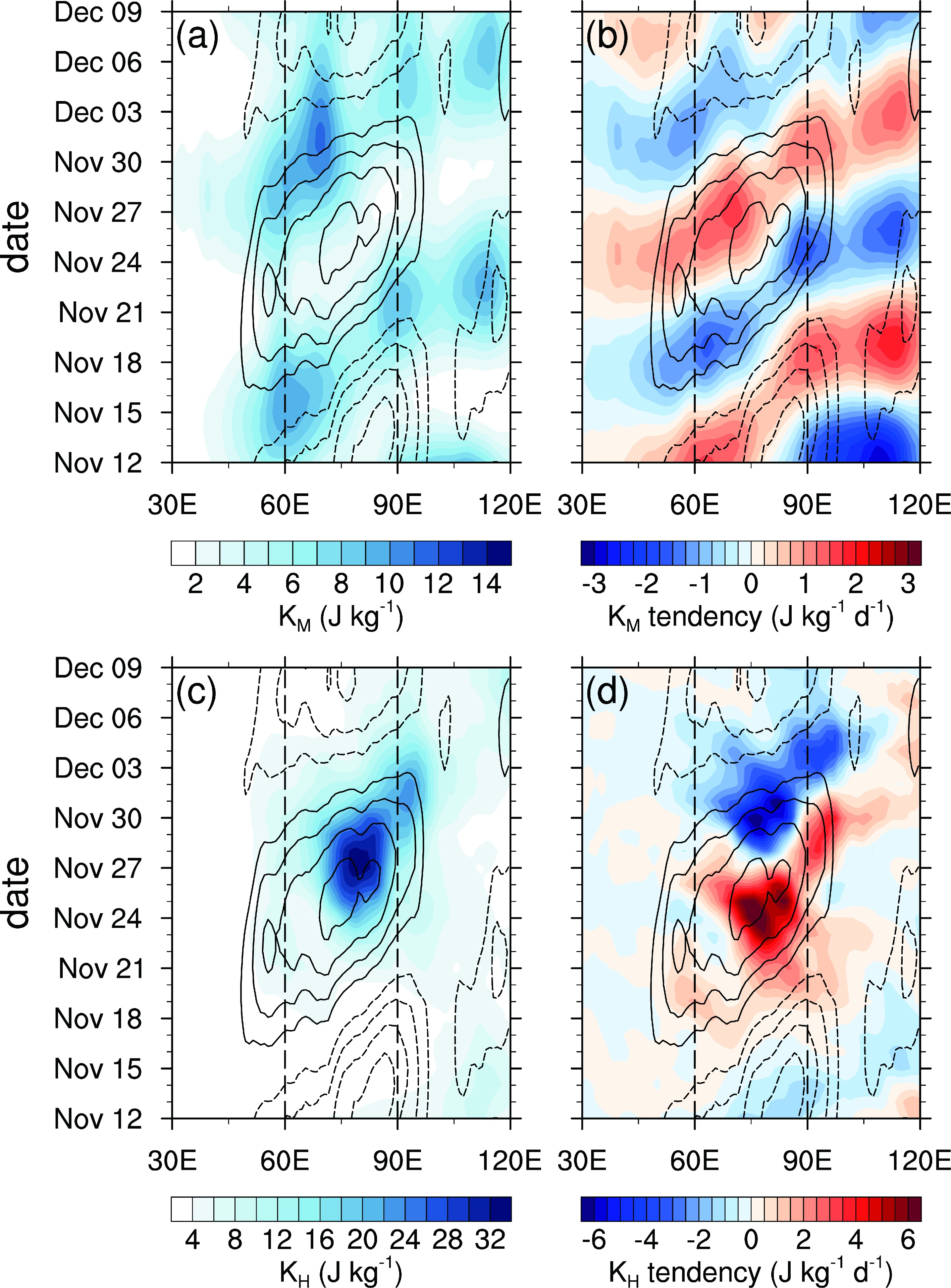 Figure3. Hovm?ller diagrams of 1000?400 hPa mass-weighted (a) mean MJO kinetic energy (color; units: J kg?1) and (b) its tendency (color; units: J kg?1 d?1), (c) high-frequency kinetic energy (color; units: J kg?1) and (d) its tendency (color; units: J kg?1 d?1) overlaid with the corresponding 20?100-day filtered OLR anomalies (contours; interval: 10 W m?2) averaged between 10°S?10°N. Dashed contours represent positive values; zero contours are omitted. Vertical dashed black lines mark the longitudinal range of the MJO convection over the Indian Ocean.
It is worth noting that the MJO KE is very weak when the MJO convection reaches its peak over the Indian Ocean, but the high-frequency disturbances are active during this period. The high-frequency KE is strong in the middle and lower troposphere (Fig. 3c). It can be seen that the high-frequency KE increases rapidly from the initiation to the peak of the MJO convection over the Indian Ocean (Fig. 3d). The westward propagation of high-frequency KE within the eastward-moving envelope of the MJO may be related to inertio-gravity waves (Houze, 2004; Zhang, 2005).
When the MJO convection reached its peak (on 26 November 2011) over the Indian Ocean, the lower tropospheric MJO KE had two maximum centers along the equator (Fig. 4a). One is located over the western Indian Ocean, dominated by the lower-level MJO westerlies. The MJO KE here will continue to strengthen that indicated by the positive MJO KE tendency. The other is located near the Maritime Continent dominated by MJO easterlies in the lower troposphere, and the MJO KE in this region will be weakened.
 Figure4. (Left column) Horizontal distributions of the 1000?400 hPa mass-weighted mean kinetic energy (color; units: J kg?1) and their tendencies (contour; units: J kg?1 d?1) as well as 850 hPa horizontal wind anomalies (vector; units: m s?1), and (right) vertical-zonal distributions of 10°S?10°N mean kinetic energy (color; units: J kg?1) and their tendencies (contour; units: J kg?1 d?1) as well as the zonal wind and vertical velocity anomalies (vector; units: m s?1) for the (top panel) MJO, (middle) high-frequency, and (bottom) low-frequency background state components on 26 November 2011. The contour interval is 0.5 J kg?1 d?1 for the MJO and low-frequency background state components, while 1 J kg?1 d?1 for the high-frequency component. Dashed contours are for negative values; zero contours are omitted. The vertical velocities are scaled by a factor of 100 to make them visible. The red box and the blue box represent the MJO kinetic energy strengthened and weakened regions, respectively. The black box denotes the high-frequency kinetic energy strengthened region.
The MJO KE shows a prominent quadrupole structure with a small value near its convective center in the troposphere for the zonal-vertical structure over the equatorial Indian Ocean (Fig. 4b). The wind fields of the MJO are featured by a baroclinic vertical structure: converging in the lower troposphere and diverging in the upper troposphere. Two maximum centers in the lower and middle troposphere are referred to as the lower tropospheric MJO KE in the following study, while the other two around the tropopause are treated as the upper-tropospheric MJO KE. Similar to the horizontal distribution (Fig. 4a), the maximum centers of lower tropospheric MJO KE are located to the west and east sides of the MJO convection center, respectively (Fig. 4b). The maximum center related to the lower-level MJO westerlies is between 400?500 hPa. In comparison, the one related to the lower-level easterlies is located around 600 hPa, much weaker than the one of the westerlies. The positive MJO KE tendency evolves from the lower to the middle troposphere, presenting a westward-tilting structure, consistent with previous research (Adames and Wallace, 2015). The MJO KE tendency in the upper and lower troposphere is positive to the west side of the MJO convection, indicating the further increase of the MJO KE in this region. During the MJO convection initiation, the westerlies gradually strengthen, so the MJO-related Rossby gyres to the west of the convection center are enhanced. The enhancement of Rossby gyres demonstrates the building up of the MJO circulation, especially to the west of its convection center. The KE tendency associated with easterlies to the east of the MJO convection is negative because the convective convergence center propagates eastward. Such a distribution of MJO KE tendency indicates that the MJO convection will move eastward.
High-frequency disturbances play an essential role in maintaining the MJO convection (e.g., Krishnamurti et al., 2016). The strong high-frequency KE is mainly located near the MJO convection center and will be further enhanced due to the positive tendency (Fig. 4c). In the vertical direction, the high-frequency KE is mainly concentrated in the lower troposphere with a maximum center at about 700 hPa (Fig. 4d). The high-frequency KE shows an increasing trend over a large area of the Indian Ocean below 250 hPa. Simultaneously, a relatively narrow area is dominated by strong high-frequency KE around 80°E, corresponding to the strong high-frequency vertical upward motion. Compared with MJO and high-frequency KE components, the LFBS KE is much weaker in the tropics, and it is dominated by upward motion and upper tropospheric easterlies over the Indian Ocean (Figs. 4e, f).
To further explore the reasons for the evolution of MJO and high-frequency KE, the physical processes that induced the change of MJO and high-frequency KE components are analyzed. One of the dominant energy sources for the MJO KE tendency is the energy converted from MJO APE


 Figure5. Pressure-longitude diagrams of 10°S?10°N mean kinetic energy tendencies (contours; units: J kg?1 d?1) and their components (color) due to (a, f) the conversion from available potential energy, (b, g) the work done by the pressure gradient force, (c, h) kinetic energy flux divergence, (d, i) conversion from the interaction with low-frequency background state, and conversion from the interaction with (e) high-frequency and (j) MJO for the (left column) MJO and (right) high-frequency kinetic energy components on 26 November 2011. Dashed contours are for negative values; zero contours are omitted. The contour interval is 0.5 J kg?1 d?1 for the MJO component, while 1 J kg?1 d?1 for the high-frequency component. Black dashed lines denote the longitudinal range of the MJO convection over the Indian Ocean.
For the high-frequency KE, the conversion of APE to KE [


The high-frequency winds transport high-frequency KE [

In the MJO KE strengthening region (10°S?10°N, 50°?80°E), the conversion from MJO APE to KE [


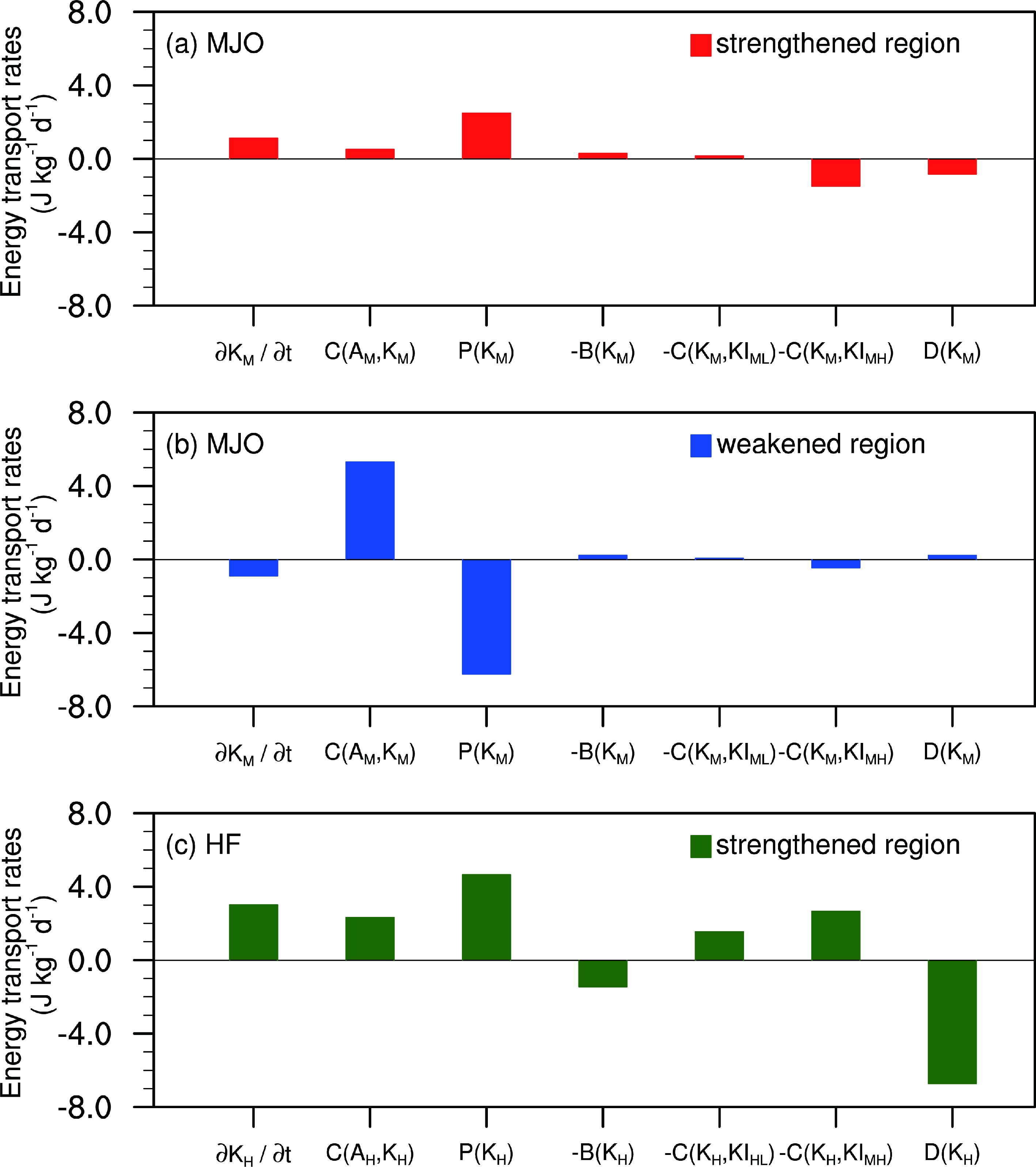 Figure6. The MJO kinetic energy tendency budget over the MJO kinetic energy (a) strengthened region (10°S?10°N, 50°?80°E) and (b) weakened region (10°S?10°N, 80°?100°E), and (c) the high-frequency kinetic energy budget over the high-frequency kinetic energy strengthened region (10°S?10°N, 60°?90°E) on 26 November 2011. All variables (units: J kg?1 d?1) are mass-weighted averaged from 1000 to 400 hPa.
The budget of the high-frequency KE in the lower troposphere (1000?400 hPa) is also analyzed over the high-frequency KE enhancement region (10°S?10°N, 60°?90°E) where the MJO convection prevails. High-frequency APE is converted into high-frequency KE, and the work done by PGF also promotes the development of high-frequency disturbances over the MJO convection center. On average, high-frequency winds transport high-frequency KE out of the MJO convection envelope, which tends to decrease the high-frequency KE over this area. However, the high-frequency disturbances gain KE when interacting with the LFBS and get more KE from the interactions with the MJO. The two-way interaction between the MJO and high-frequency disturbances indicates a downscaling energy cascade in the lower troposphere. This result is consistent with the findings that the synoptic-scale systems communicate with the MJO via a nonlinear energy transfer (Krishnamurti et al. 2016). The direct KE delivery from the MJO to the high-frequency disturbances helps organize and maintain the high-frequency disturbances, contributing to the MJO multi-scale convective envelope in return.
2
4.2. Multi-scale energy interactions
The KE budget analysis of MJO and high-frequency disturbances reveals that the MJO transmits KE to the high-frequency disturbances within the MJO convection envelope. As mentioned in section 2, the energy conversion between two different time scales does not share the same number and opposite signal in the local energy interaction system. Their sum equals the divergence of the interaction energy flux [
In the early development stage of MJO II convection, the MJO KE is very weak (Fig. 7a). Its tendency is negative (Fig. 7b), indicating that the MJO KE weakens during this period. It is not until the MJO convection began to decline over the Indian Ocean that the MJO KE gradually increased. The high-frequency KE began to grow about two days before the MJO convection was organized (Fig. 7b) and enhanced continuously in the strengthening stage of the MJO convection over the Indian Ocean. The tendency of high-frequency KE reached its peak on the day of the MJO convection reached its maximum over the Indian Ocean and began to decrease in the weakening stage of the MJO convection. There is a phase difference of about ninety degrees between the time evolution of the MJO KE tendency and the high-frequency KE tendency. To explore the relationship between the variation of MJO KE and high-frequency KE, the KE conversion between the MJO and the high-frequency disturbances is evaluated. The MJO loses KE when it interacts with the high-frequency disturbances, that is, the MJO transfers KE to the interacting energy


 Figure7. Time series of 1000?400 hPa mass-weighted mean (a) kinetic energy (units: J kg?1), (b) their tendencies (units: J kg?1 d?1), and (c) the kinetic energy conversion rate (units: J kg?1 d?1) with interaction energy KIMH for MJO (red) and high-frequency (blue) overlaid with the 20?100-day filtered OLR anomalies (grey dash line; units: W m?2) averaged over the tropical Indian Ocean (10°S?10°N, 60°?90°E).
In the local interaction between the MJO and high-frequency disturbances, the process of energy cascading not only happens in the same grid, but it can happen in different regions through the flux of the interaction energy. The interaction energy flux equals zero when the wind field of MJO and high-frequency disturbances are spatially uniform or integrate globally. During the interaction with the high-frequency disturbances, the MJO loses KE over the western Indian Ocean and Maritime Continent where the MJO lower-level zonal wind is strong, while it obtains energy through upscale energy cascades at the eastern edge of the positive MJO KE tendency (Fig. 8a). High-frequency disturbances mainly obtain KE through interacting with the MJO over the MJO convection center (Fig. 8b). The KE lost by the MJO over the western Indian Ocean and Maritime Continent can be transported into the center of the MJO convection area through the divergence of the interaction energy flux

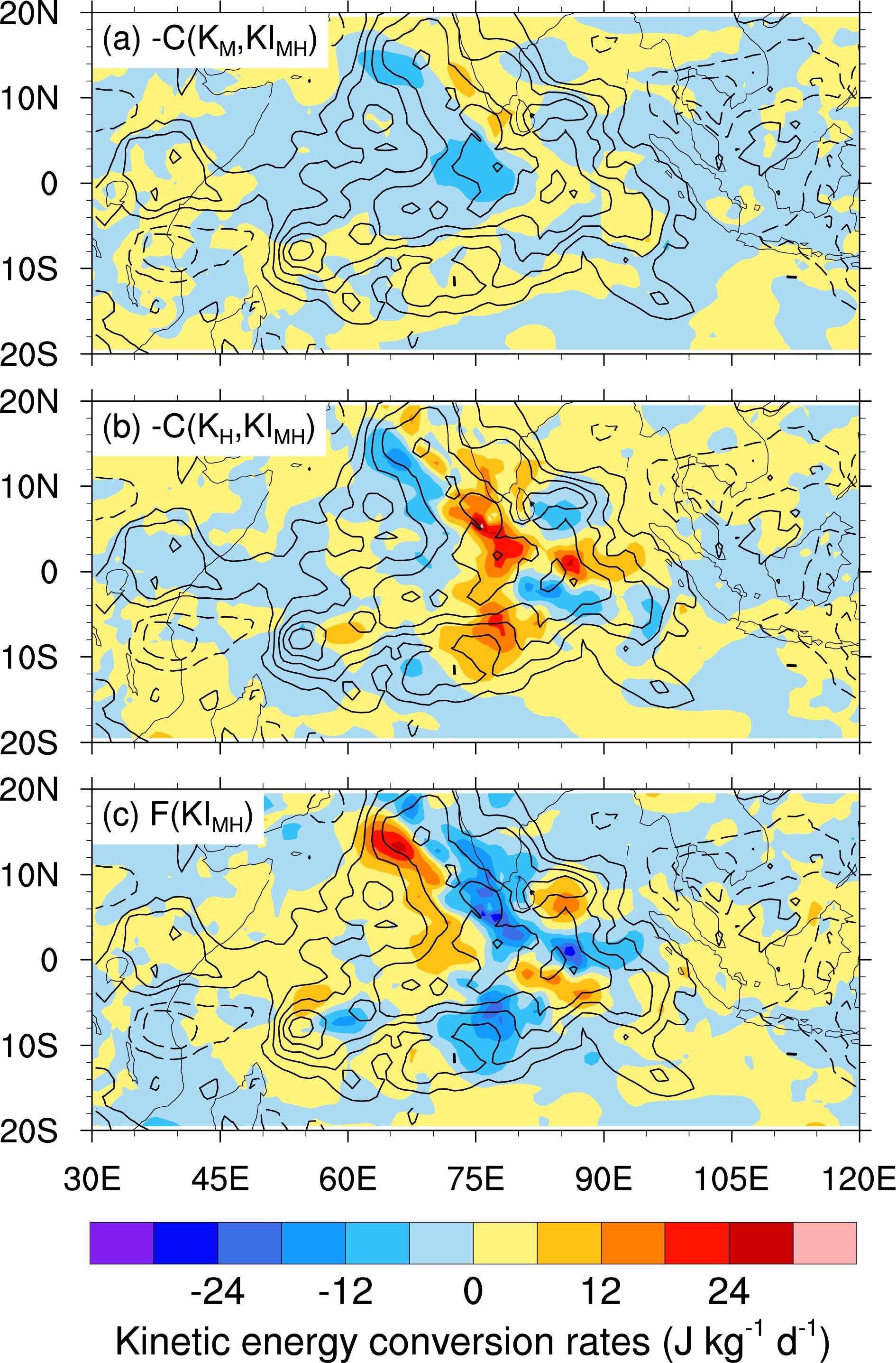 Figure8. Horizontal distributions of 1000?400 hPa mass-weighted mean kinetic energy conversion rates (color; units: J kg?1 d?1) from (a) MJO and (b) high-frequency to interaction energy KIMH, and (c) flux divergence of KIMH overlaid by the 20?100-day filtered OLR anomalies (contour; units: W m?2; interval: 10 W m?2) on 26 November 2011. Dashed contours are for positive values; zero contours are omitted.
The physical processes related to the KE tendency in the lower troposphere for this MJO are summarized in the sketch in Fig. 9 when its convection prevails over the Indian Ocean. In this MJO event, the MJO KE tendency is mainly governed by the work done by the pressure gradient force (PGF) at the MJO scale and the energy conversion from the MJO available potential energy (APE). This agrees with the view that the large-scale wind perturbation related to the MJO can be regarded as a quasi-steady response to a slowly varying heat source (Sobel and Maloney, 2012; Zhou et al., 2012). On average, the APE of the MJO is converted to KE within the MJO convection envelope in the lower troposphere. The work done by the PGF mainly increases the MJO KE in the westerly region to the west of the MJO convection and weakens the MJO KE in the easterly region. There are still some other processes that can impact the MJO KE. The advection of the MJO KE by the MJO scale winds enhances the MJO KE over the MJO convection region. In interactions with other time scales, the MJO can obtain a small amount of KE through interacting with the low-frequency background state (LFBS), while the MJO tends to dissipate the KE through interacting with the high-frequency disturbances in the lower troposphere. The energy transport and conversion process related to the MJO in the upper troposphere (400?200 hPa) are quite different from those in the lower troposphere. The release of convective heating in this layer creates upward movement inside the MJO convection, promoting the MJO APE converted into KE in large quantities, but the work done by the PGF mostly offsets this effect. The MJO winds transport MJO KE out of the MJO convection area in the upper troposphere. The interaction between the MJO and LFBS plays an essential role in decelerating MJO winds in the upper troposphere. The upscale energy transmission is identified in the upper troposphere, and the energy conversion between MJO and high-frequency disturbances replenishes MJO KE in the upper troposphere.
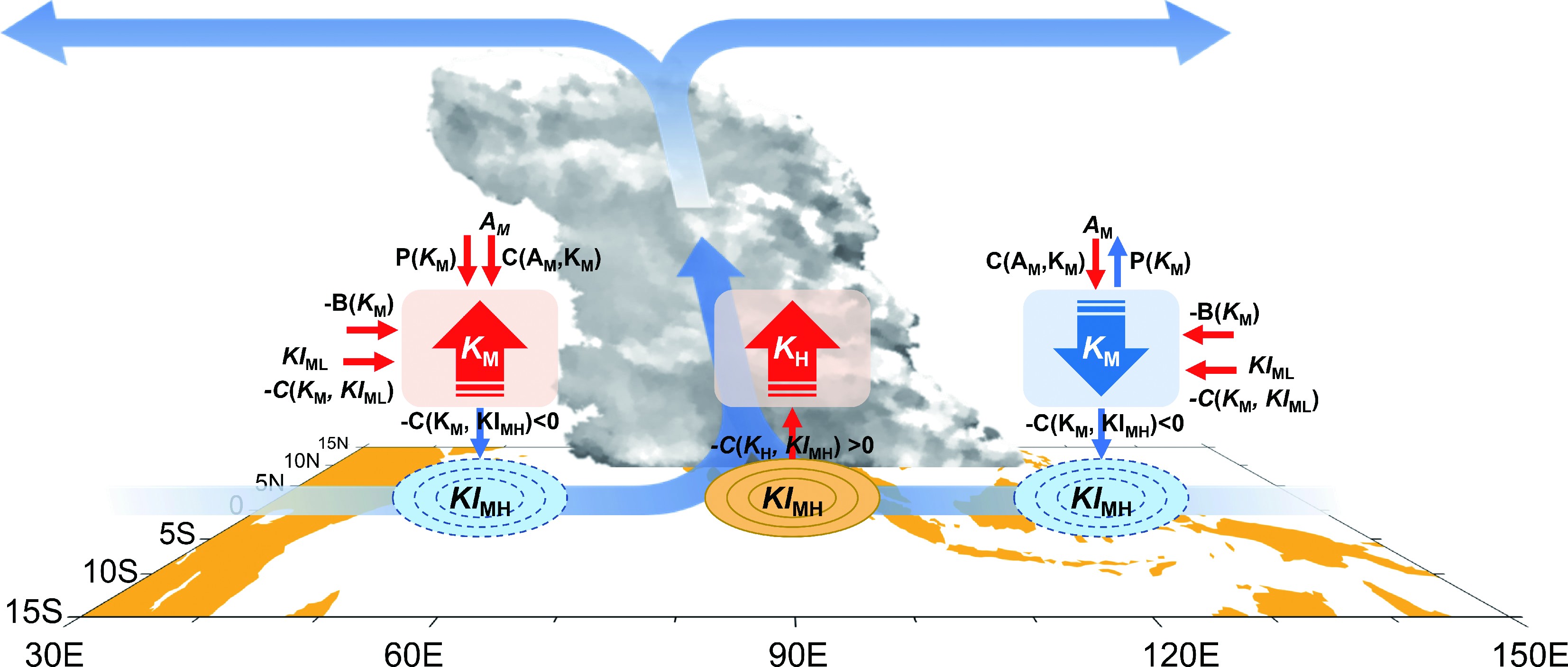 Figure9. Sketch for the MJO kinetic energy transportation path on 26 November 2011 over the Indian Ocean. The cloud pattern represents the MJO convection. The squares represent the positive (red) and negative (blue) energy tendency centers. Correspondingly, the thick arrows inside the squares indicate the increase (blue) or decrease (red) of corresponding kinetic energy. The orange and blue ellipses represent the flux convergence and divergence of interaction energies, respectively. The red and blue solid arrows indicate the inward and outward energy transfer, respectively. The blue gradient arrows indicate the MJO circulations.
The local three-scale energy budget framework developed in this study allows us to reveal the complete energy transport path related to the MJO and display the energy conversion between the MJO and high-frequency disturbances and between the MJO and LFBS. The results show that the interaction between the MJO and LFBS in the lower troposphere is relatively weak, but it contributes to the strengthening of the MJO westerlies that enhance convergence in the lower troposphere. Because the high-frequency convection is usually located in the lower troposphere and its interaction with the MJO is also strong there, the interaction between MJO and high-frequency disturbances in the lower troposphere (1000?400 hPa) is further discussed. According to the analysis in section 4, both


The MJO KE is of small amplitude near the MJO convection center, but the MJO circulation plays an important role in organizing the high-frequency convective complexes within the convection envelope. The intensity of convection within the MJO envelope is directly affected by the intensity of high-frequency disturbances. This result is consistent with the previous study that the tropical intraseasonal oscillation strengthens the synoptic disturbances (Maloney and Dickinson, 2003). The increase of high-frequency KE will lead to the enhancement of high-frequency disturbances. The latent heating released from those high-frequency disturbances will provide the energy for developing and maintaining the MJO circulation. The feedback of the high-frequency disturbances to the MJO could be through the scale interaction of available potential energy transfer between the MJO and high-frequency systems, which is beyond the scope of this study. The interaction between high-frequency disturbances and the MJO plays an important role in maintaining the high-frequency disturbances within the MJO convection envelope, which is conducive to maintaining MJO convection and then the MJO circulation.
The KE budget analysis in a local multi-scale interaction framework is attempting to derive the dynamical mechanisms of MJO. By applying this framework to a typical MJO event during DYNAMO, the KE transport path of this MJO event shares certain common features with the previous studies (e.g., Zhou et al., 2012), indicating the feasibility of this method. This approach provides a possible way to investigate the evolution of the energy transport path during the life cycle of MJO, especially the differences in the energy transport path when MJO convection is over the Indian Ocean, Maritime Continent, and western Pacific. In a future study, it would be worthwhile to apply this KE budget analysis to the multiple MJO events using high-resolution reanalysis data to obtain the general picture of the MJO energy transport path.
Acknowledgements. The authors thank two anonymous reviewers for their constructive comments that help improve the manuscript. This study was supported by the National Key R&D Program of China through Grant Nos. 2018YFC1505901 and 2018YFA0606203, the National Nature Science Foundation of China through Grant Nos. 41922035, 41575062, 41520104008, Key Research Program of Frontier Sciences of CAS through Grant No. QYZDB-SSW-DQC017, and the Youth Innovation Promotion Association, Chinese Academy of Sciences. The first author acknowledges the support from the China Scholarship Council (CSC) Grant No. 201904910516.
