Bin LIU^1,2,3,
Zhenghui XIE^1,3,,,
Peihua QIN¹,
Shuang LIU⁴,
Ruichao LI^1,3,
Longhuan WANG^1,3,
Yan WANG^1,3,
Binghao JIA¹,
Si CHEN^1,3,
Jinbo XIE¹,
Chunxiang SHI⁵

Corresponding author: Zhenghui XIE,zxie@lasg.iap.ac.cn;

1.State Key Laboratory of Numerical Modeling for Atmospheric Sciences and Geophysical Fluid Dynamics, Institute of Atmospheric Physics, Chinese Academy of Sciences, Beijing 100029, China
2.School of Software Engineering, Chengdu University of Information Technology, Chengdu 610103, China
3.University of Chinese Academy of Sciences, Beijing 100049, China
4.Key Laboratory of Mountain Hazards and Earth Surface Processes, Institute of Mountain Hazards and Environment, Chinese Academy of Sciences, Chengdu 610041, China
5.National Meteorological Information Center, China Meteorological Administration, Beijing 100081, China
Manuscript received: 2020-05-13
Manuscript revised: 2020-08-21
Manuscript accepted: 2020-10-09
Abstract:With economic development and rapid urbanization, increases in Gross Domestic Product and population in fast-growing cities since the turn of the 21st Century have led to increases in energy consumption. Anthropogenic heat flux released to the near-surface atmosphere has led to changes in urban thermal environments and severe extreme temperature events. To investigate the effects of energy consumption on urban extreme temperature events, including extreme heat and cold events, a dynamic representation scheme of anthropogenic heat release (AHR) was implemented in the Advanced Research version of the Weather Research and Forecasting (WRF) model, and AHR data were developed based on energy consumption and population density in a case study of Beijing, China. Two simulations during 1999?2017 were then conducted using the developed WRF model with 3-km resolution with and without the AHR scheme. It was shown that the mean temperature increased with the increase in AHR, and more frequent extreme heat events were produced, with an annual increase of 0.02?0.19 days, as well as less frequent extreme cold events, with an annual decrease of 0.26?0.56 days, based on seven extreme temperature indices in the city center. AHR increased the sensible heat flux and led to surface energy budget changes, strengthening the dynamic processes in the atmospheric boundary layer that reduce AHR heating efficiency more in summer than in winter. In addition, it was concluded that suitable energy management might help to mitigate the impact of extreme temperature events in different seasons.
Keywords: anthropogenic heat release,
extreme temperature event,
Weather Research and Forecasting model,
Beijing
摘要:21世纪以来，快速发展的经济和城市化增加了人口与GDP，能源消耗快速增加。由此产生的人为热释放到近地表大气，引发城市热环境的改变及极端温度事件的频发。为探究能源消耗对城市极端温度事件（包括极端高温和低温事件）的影响，本文以北京市为例，构建了基于能源消耗和人口密度的人为热数据集，并在WRF模式中实现了人为热参数化方案的动态表达。基于改进后的模式，本文分别开展了有人为热影响和没有人为热影响的两组模拟试验，模拟时间为1999年至2017年，空间分辨率为3km。结果表明：人为热排放的增加导致平均气温升高；基于7个极端温度指标，极端热事件发生频率增加，年增加量为0.02～0.19天；极端低温事件降低，年减少量为0.26～0.56天。这主要因为人为热通过感热通量引起地表能量收支变化，增强了边界层的动力过程，使夏季人为热的加热效率低于冬季。同时还表明，适当的能源管控可能有助于缓解不同季节极端温度事件的影响。
关键词:人为热,
极端温度事件,
WRF模式,
北京

HTML

--> --> -->

The level of urbanization has increased from 39% to 55% in the last four decades globally (Chen et al., 2014b; United Nations, 2018). Vast numbers of people move from rural areas to urban areas across the world with about 2% energy consumption growth annually during the 21st century (Enerdata, 2018). Anthropogenic heat flux is mainly released from energy consumption supporting residents’ accommodation and transportation, leading to changes in the urban thermal environment and extreme heat events (Feng et al., 2012; Chen et al., 2014a). Anthropogenic heat release (AHR) increases the occurrence of extreme temperature by heating the surface atmosphere directly (Salamanca et al., 2014) and functions as the main factor in the urban heat island effect, which has synergistic interactions with heat waves (Zhao et al., 2018; Rizvi et al., 2019). The number of extreme temperature events in the first decade of the 21st century grew faster than in the last 10 years of the 20th century (WMO, 2013). From the news report of Beijing of China on 3 August 2018, the number of hot days up to that date had already exceeded the total number of hot days in 2017, and the temperature reached a maximum of 42.1°C (Sina, 2018). Besides, increased temperatures can substantially increase the rate of temperature-related illnesses (Schr?ter et al., 2005; Jenerette et al., 2011; Tian et al., 2012; Zhang et al., 2014) and impose a heavy water supply burden on the urban ecosystem (Huang et al., 2010; Jenerette et al., 2011). Understanding and quantifying the influence of AHR on urban climate and extreme temperature events is an important component of urban energy management (Wang et al., 2013).
Previous studies have focused mainly on the weather and short-term climate effects of AHR, including daily and seasonal impacts. AHR is significantly positively correlated with the urban heat island effect (Basara et al., 2010; Du et al., 2016) and raises temperatures by about 0.5°C?1°C in urbanized areas, an effect that is more pronounced in winter than in other seasons (Wilby, 2003; Feng et al., 2014; Wang et al., 2015). The influence of AHR is greater at night than in the daytime (Narumi et al., 2009; Mohan et al., 2012; Schrijvers et al., 2015), producing a greater increase in temperature, and the contribution of AHR among all warming factors increases to 75% at 0800 LST (Wang et al., 2013). For a specific intense heat wave event, AHR plays a key role in the synergies between the urban heat island effect and heat waves (Founda and Santamouris, 2017; Zhao et al., 2018; Rizvi et al., 2019). According to studies of extreme temperature events, the changes in extreme temperature events are mostly related to greenhouse gas concentrations, anthropogenic aerosols, land-use change, and so on (Wen et al., 2013), but there has been a lack of consideration of AHR from energy consumption despite it being a key human activity in urban areas. Besides, extreme temperature events induced by AHR change the long-term frequency and trend of extreme temperature events, a phenomenon that deserves more attention but is rarely considered by meteorologists. Although AHR contributes only about 0.3% of the total heat flux at a global scale (Basara et al., 2010), its effect is increasing and very large in specific regions. Taking London and Tokyo as examples, the values of AHR have been estimated to be 10.9?1590 W m^?2 (Ichinose et al., 1999; Iamarino et al., 2012). In Beijing, rapid changes in AHR have altered the surface energy balance much more than the Chinese average (Chen et al., 2012; Yu et al., 2014). Therefore, it is appropriate to regard Beijing as a case for studying the influence of AHR on extreme temperature events, but there are some difficulties in using observational or model data based on case studies. Existing AHR data are either too low in resolution or too short-term (Chen et al., 2012; Dong et al., 2017). Determining the temporal and spatial variation of AHR in line with regional economic development and energy consumption is essential to reveal the effect on long-term climate and extreme temperature events. The Weather Research and Forecasting (WRF) model, which is based on fixed diurnal profiles of anthropogenic heat, is a good tool for research on climate effects but lacks a dynamic representation scheme for land?atmosphere interaction and does not consider abrupt temperature changes due to the effect of human activities (Dong et al., 2017).
Recently, geoengineering strategies like increasing the albedo of urban roofs, implementation of green infrastructure, and using highly reflective paint for road pavements (Yaghoobian and Kleissl, 2012; Wang et al., 2013; Norton et al., 2015) have been regularly shown to be effective ways to cool cities, but may not help to warm cities when extreme cold events occur. Engineers focus on these operational methods to reduce heat or cold stress risks, but give less consideration to the influence of energy consumption on climate. Anthropogenic heat flux is closely related to energy consumption, which is the main factor in urban heat island intensity and heat wave events (Ryu and Baik, 2012). Energy consumption adjustments can provide another way to deal with extreme temperature events from the perspective of AHR.
This work aims to reveal the long-term frequency and trend of extreme temperature events caused by AHR from energy consumption in a case study of Beijing during the 21st century, and reveal the influences of AHR on extreme temperature events over long periods, which might provide advice to urban planners trying to mitigate extreme temperature events. Then, we discuss whether the study methods can be applied to other cities. Here, temporal and spatial AHR data for Beijing from 1999 to 2017 were gathered for the case study, and the corresponding modifications to the AHR scheme in the WRF urban canopy model (UCM) were made to start the simulations.
The rest of this paper is structured as follows: Section 2 describes the model development, including a new AHR scheme considering the influence of abrupt temperature changes on anthropogenic heat flux. Section 3 discusses the data and the experimental design. Section 4 presents the effects of AHR on extreme temperature events, including AHR variation, model validation, the frequency and trend of extreme heat events, and the mechanism relating AHR to extreme temperature events. Concluding remarks are given in section 5.

As part of the sensible heat flux, AHR upsets the raw energy balance. Equations (1) and (2) represent the energy balance equation without and with AHR, respectively. Once AHR increases are incorporated into the energy balance, the net radiation flux transferred from the urban land surface to the atmosphere also increases:
and
where ${\rm{Rn}}$, ${\rm{LE}}$, $ H $, G and $ {\rm{AHR}} $ represent the net radiation flux, latent heat flux, sensible and ground heat flux, and anthropogenic heat flux from the urban land surface to the near-surface atmosphere. The subscripts “no-AHR” and “AHR” represent the energy balance without and with AHR, respectively. In the default scheme of the WRF model, the AHR (denoted as $ {\rm{AHR}}_{\rm{default}} $) is the product of the maximum AHR ($ {\rm{AHR}}_{\rm{max}} $) and the empirical diurnal profile [$f(h) $] without spatial differences. AHR in this paper ($ {\rm{AHR}}_{\rm{new}} $) is a spatiotemporal variable that changes according to latitude and longitude, as well as yearly, monthly and daily. The climatological and abrupt temperature changes are also considered, showing the increasing release of AHR when the weather is very cold or very hot:
where $ {\rm{AHR}}_{\rm{default}} $, $ {\rm{AHR}}_{\rm{new}} $, and $ \overline {{\rm{AH}}{{\rm{R}}_{i,j}}} $ are the default AHR, newly adopted AHR, and average grid cell AHR, respectively, where the subscripts “i” and “j” represent the latitude and longitude; y, m, h, T, and $ \overline T $ indicate the year, month, hour, current temperature, and many-year average temperature, respectively; $ {g_1}(y) $, ${g_2}(m)$, and ${g_3}(h)$ represent the function of year (y), month (m), and hour (h); $ {g_4}(T,\overline T)$ is a function of current temperature ($ T$) and climatological temperature ($\overline T $), which is assumed to have a linear relationship with the absolute value of the temperature difference, as shown in Eq. (6), where a and b are assumed to be 0.1 and 5, respectively; and f(h) is a fixed empirical diurnal profile that varies hourly. This function has an “M” shape and reaches its maximum at 0900 and 1700 LST.
The WRF model is a limited-area, nonhydrostatic, mesoscale modeling system with a terrain-following eta coordinate, coupled with a UCM to provide a better representation of the physical processes involved in the exchange of heat, momentum, and water vapor in an urban environment. The UCM is a single-layer model with a simplified urban geometry. Some of its features include shadowing from buildings, reflection of short- and longwave radiation, the wind profile in the canopy layer, and multi-layer heat transfer equations for roofs, walls, and road surfaces (Tewari et al., 2007). Anthropogenic heat is optional in urban environmental simulations, which are based on fixed AHR values according to urban types. For example, the daily maximum AHR values are 90, 50 and 20 W m^?2 for high-, middle- and low-density urban areas in the default AHR scheme. An empirical diurnal profile is used to represent the daily variation in anthropogenic heat flux in the single-layer model. The advanced AHR scheme mentioned above was coupled into the WRF model (see Fig. 1). AHR is regarded as part of the sensible heat flux and changes the energy interaction by upsetting the energy balance between the land surface and the atmosphere. In addition, climatological temperature and AHR gridded data were input into this scheme by a data interface of the WRF model when conducting initialization of real-time case, and the current temperature was from each step of the model output.
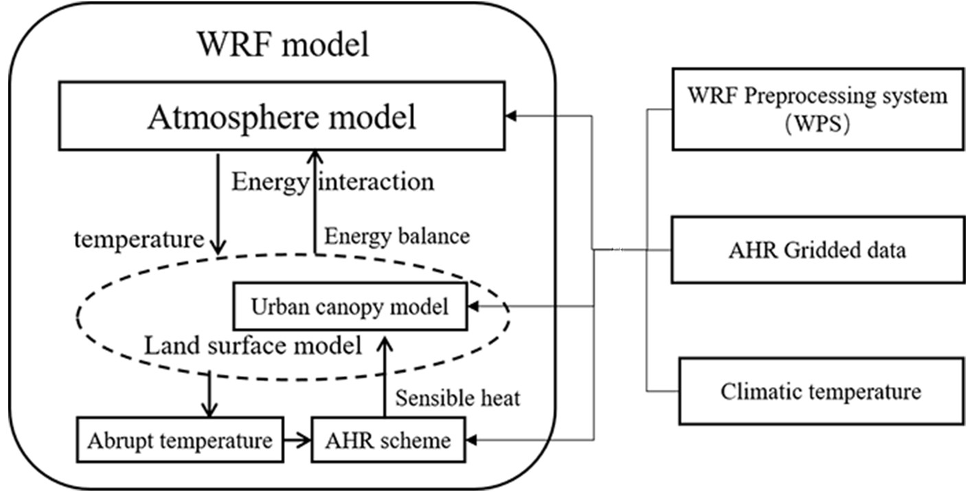Figure1. Schematic diagram of the anthropogenic heat scheme coupled with the WRF model.

2

-->

3.1. AHR

AHR can be divided into four components (AHR from vehicles, the building sector, industry, and human metabolism) (Sailor and Lu, 2004), representing the major sources of waste heat in the urban environment, as shown in Eq. (7):
where $ Q_{\rm{V}} $, $ Q_{\rm{B}} $, $ Q_{\rm{I}} $ and $ Q_{\rm{M}} $ represent the AHR from vehicles (V), the building sector (B), industry (I), and human metabolism (M). Human metabolic rates are not constant over the course of a day, and normally metabolic heat flux accounts for less than 1 W m^?2 of the total anthropogenic heat and can therefore be ignored (Grimmond, 1992; Sailor, 2011). Hence, in this paper, metabolic heat flux is not included in the total AHR. Because anthropogenic heat is closely tied to energy consumption (Sailor, 2011), the AHR from vehicles, buildings, and industry can be estimated by listing all kinds of energy consumption. Hence, AHR can be estimated by the following function:
where $ {E_k} $ represents the kth kind of energy consumption (with the subscripts denoting coal, coke, crude oil, gasoline, kerosene, diesel, fuel oil, natural gas, and electric power) and $ {a}_{k} $ is the heat release coefficient of the kth kind of energy consumption. Hence, AHR can be represented by nine kinds of energy consumption. However, the energy consumption of Beijing is recorded by the National Bureau of Statistics and released yearly in a form that is incompatible with the grid resolution of the model simulation. Hence, the energy consumption must be downscaled to the grid size. Population density has been commonly used to map total energy consumption to different spatial scales (Washington, 1972; Block et al., 2004), including the energy consumption of Beijing for nine kinds of energy from 1999 to 2017. Empirical monthly profiles of Beijing’s AHR were extracted from a global anthropogenic heat flux database with a high spatial resolution of 30 arc-seconds and a temporal resolution of 1 h (Dong et al., 2017), which was based on gridded monthly temperatures derived from various measurements and radiance-calibrated nighttime lights. The monthly profiles showed spatial variations and were convincing, but the time period of the raw data was limited to one year, which could not meet the research needs of this paper. The calculation was performed as in Eq. (9), and a schematic of the AHR methodology is shown in Fig. 2:
Figure2. Flowchart of AHR data estimation.


where $ {\rm{POP}}_{i,j} $ is the gridded population density, where the subscripts “i” and “j” represent the latitude and longitude, $ {\rm{AHR}} $ is the total anthropogenic heat flux, and $ \overline{{\rm{AHR}}_{i,j}} $ is the average grid AHR downscaled by population density.

2 -->

3.2. Data

Air temperature and wind speed data for Beijing from observation and reanalysis datasets were used for model validation (Table 1). In this paper, observed temperature data from 20 national meteorological stations in Beijing and wind speeds from 205 non-watching automatic weather stations were used. The regional reanalysis data came from the China Meteorological Administration Land Data Assimilation System (CLDAS) as hourly outputs with a resolution of 0.0625° × 0.0625°. Regional and site observations of temperature comparisons were carried out to verify the effectiveness of the WRF physical schemes and determine whether these schemes were reasonable for long-term urban simulation with the new AHR scheme. This paper mainly focuses on comparing AHR simulation results with reanalysis data and in-situ data.

Scale	Variables	Resource	Other aspects
Site	Temperature	National meteorological stations	20 observation sites; hourly; 2001?17
	Wind speed	Automatic weather stations	205 observation sites; hourly; Dec 2008 to Dec 2010
Regional	Temperature and wind speed	CLDAS	0.0625° × 0.0625°; hourly; 2008?14

Table1. Dataset descriptions.



2 -->

3.3. Experimental design in the case study

The Advanced Research version of the WRF model (Skamarock et al., 2008) dynamic core, version 3.9.1, coupled with a single-layer UCM was used in the experiments in this study. Two kinds of experiments were performed, with and without AHR (denoted “AHR” and “no-AHR”, respectively, in this paper). In the AHR experiment, the AHR data were regarded as a new input variable by adding them to the model initial input files with the same spatial resolution as the model and replacing the raw files once the model was running. Other variables, like many-year averaged air temperature and monthly profiles of the spatial distribution, were input from the initial files to calculate the hourly AHR for a specific year and day. AHR was treated as part of the sensible heat flux in this model, transferring to the near-surface atmosphere and upsetting the normal energy balance.
In this study, two-layer nested domains with horizontal resolutions of 15 km (d01; mesh size 121 (lon) × 144 (lat), most of northern China), 3 km (d02; mesh size 206 (lon) × 251 (lat); almost all the Jing-Jin-Ji metropolitan area, and Beijing as the area of interest), were designed for these experiments (Fig. 3). NCEP FNL 6-h data (including soil water, moisture, and temperature) were used for the first-guess initial field and lateral boundary conditions. SSTs were needed to run long-term simulations, for which the OISST high-resolution dataset (daily, 0.25° × 0.25°) was chosen in this study. The terrestrial and MODIS land-use data provided in the WRF model described the real terrestrial and land-cover characteristics of the regions of interest, and the default static data were used in the experiments. The simulation period ran from 1 December 1999 to 31 December 2017. The first year, from December 1999 to December 2000, was considered as an initialization period. Two-meter air temperature data from 2001 to 2017 were used for further analysis of the model outputs for each hour. In terms of physical options, the schemes described in Table 2 were used.

Physical scheme	Selected scheme option
Microphysics	Kessler scheme
Longwave	RRTM scheme
Shortwave	MM5 shortwave scheme
Cumulus	Grell?Devenyi
Planetary boundary physics	ACM2 PBL scheme
Land surface model	NOAH-MP
Urban model	SLUCM

Table2. Physical parameterization schemes.


Figure3. Simulation area with two domains. The left-hand panel shows that D01 covers North China mostly, and the right-hand panel shows the position of D02 nested in D01, the color bar represents topography height.

2

-->

4.1. Model validation

Compared with the seven-year (from 2008 to 2014) average temperature in the CLDAS and AHR simulation results shown in Fig. 4, both temperatures in the city center were higher than in the suburbs. The similar spatial distributions show that the WRF physical scheme is reasonable. The correlation coefficients between the CLDAS temperatures and the AHR simulation results were mostly quite close to one, and the average root-mean-square error (RMSE) of the two datasets was 0.8°C. The gridded model results were interpolated to the site according to the coordinates of stations in both urban and suburban areas, and comparisons between site observations and AHR simulation results also showed that the simulation results for temperature were in good agreement with observations (Fig. 4b). Table 3 gives the regression coefficients, RMSE, and square of the correlation. There were nine stations on six ring roads and 11 stations in the suburbs. The results show that the AHR simulation results are reasonable, with simulated temperatures slightly higher than observations and RMSEs less than 2.5°C. Also, 10-m wind speed comparisons were conducted (see Fig. 5). Compared with CLDAS analysis data, and 205 non-watching automatic weather stations, the correlation coefficients are mostly larger than 0.6, and the RMSE is less than 1.3 m s^?1, showing the AH simulation had good agreement with both CLDAS data and observations.

No.	Coordinates	RC	RMSE	R2	No.	Coordinates	RC	RMSE	R2
1	(39.98°N, 116.28°E)	1.099	2.638	0.978	11	(40.6°N, 116.13°E)	1.038	2.853	0.982
2	(39.95°N, 116.2°E)	1.092	2.31	0.978	12	(40.45°N, 115.97°E)	1.044	1.758	0.982
3	(39.92°N, 116.12°E)	1.09	2.58	0.96	13	(40.22°N, 116.22°E)	1.098	2.066	0.983
4	(39.87°N, 116.25°E)	1.09	2.351	0.977	14	(40.65°N, 117.12°E)	1.058	1.699	0.986
5	(39.95°N, 116.48°E)	1.093	2.25	0.979	15	(40.37°N, 116.63°E)	1.090	2.051	0.98
6	(39.8°N, 116.47°E)	1.10	1.918	0.984	16	(40.38°N, 116.87°E)	1.074	1.969	0.983
7	(39.75°N, 116.33°E)	1.102	2.138	0.982	17	(40.15°N, 117.1°E)	1.062	2.584	0.98
8	(39.72°N, 116.63°E)	1.112	2.028	0.977	18	(39.97°N, 115.68°E)	1.020	1.954	0.975
9	(40.13°N, 116.62°E)	1.10	2.062	0.984	19	(39.73°N, 115.73°E)	1.071	2.153	0.98
10	(40.73°N, 116.63°E)	1.009	2.235	0.981	20	(39.7°N, 116.0°E)	1.094	2.013	0.982

Table3. Regression coefficients (RCs), RMSE, and square of the correlation (R²) of observed and AHR simulated temperatures.


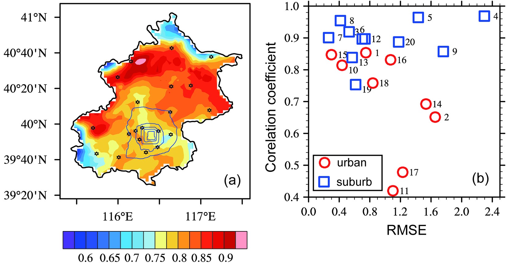Figure4. Comparison between observed and simulated values: (a) correlation coefficients of yearly temperatures between CLDAS and AHR simulation; (b) RMSE and correlation coefficients of temperature between observation and AHR simulation. The observation stations can be seen in Table 3.


Figure5. Wind speed comparisons between observed and simulated values: (a) spatial distribution of temporal correlation coefficients between CLDAS reanalysis data and AHR simulations; (b) correlation coefficients and RMSEs between station observations and AHR simulations, where the sizes of circles denote the values of correlation coefficients and the colors represent the RMSE.



2 -->

4.2. Frequency and trend of extreme temperature events in the case study

In the approach proposed here, daily average AHR is mainly based on energy consumption and population density, which both have spatial distributions. Most AHR is concentrated within the six ring roads of Beijing (see Fig. 6a), with maximum values greater than 80 W m^?2 in the city center; in the suburbs, the AHR is less than 2 W m^?2. In yearly terms, from Fig. 6b, due to Beijing’s energy management for environmental protection, high-energy industries have moved to other provinces or have moved away from using dirtier forms of energy, such as coal and coke. Instead, environmentally friendly energy such as natural gas and electric power, along with irreplaceable energy like gasoline, are increasing rapidly. Energy upgrades are mostly conducted in the city center, with impacts on urban central heating in winter, traffic on roads, and some factories. Although dirty or clean energy consumption may increase or decrease with urban regulation, the anthropogenic heat of Beijing increased from 2001 to 2010, but after 2010, AHR became stable and reached a maximum. From the monthly variations shown in Fig. 6c, which are based on the work of Dong et al. (2017), it is apparent that AHR is higher in winter than in other seasons, which makes sense because urban central heating is used in winter to counteract low temperatures, leading to more energy consumption. Spatial differences in AHR are much greater than monthly variations, as can be seen from the bar value of each month representing the log₁₀ of spatial variations in Fig. 6c. In winter, the variations in spatial distribution are bigger than in other seasons. The estimated diurnal profiles are different due to changes in daily lifestyle pattern such as holidays and festivals. Diurnal profiles in this research were based on the default profiles, but took abrupt temperature changes into consideration according to Eq. (6), which was applied to the UCM.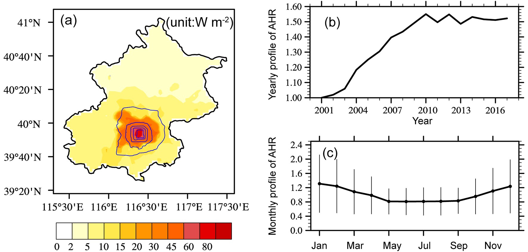
Figure6. (a) Spatial distributions of daily average AHR from 2001 to 2017. The closed curve from the inside to the outside represents the second to sixth ring roads of Beijing with high population density. (b) Yearly and (c) monthly profiles of AHR, with the bars representing the spatial standard deviation of lgAHR.


Comparing the AHR and no-AHR simulation results, the temperature differences were mainly located in the city center, with a maximum increase of 1.14°C, and there was variation among the seasons, with average increases of 0.06°C, 0.01°C, 0.11°C and 0.18°C for spring, summer, fall and winter, respectively. The frequency distribution of the temperature increase (Figs. 7f-j) shows that in suburban areas the temperature showed no increase, but in the city center it increased more because more than 90% of AHR is located within the six ring roads of Beijing, where the area of high population density is situated. There, anthropogenic heat flux release to the near-surface atmosphere heats the air directly and makes the temperature rise. From Figs. 7a-e, both frequency distributions of temperature increase show that the city center experiences a stronger effect than the suburbs. The yearly and four seasonal average temperature increases were 0.525°C, 0.362°C, 0.191°C, 0.621°C and 0.936°C, respectively, with seasonal temperature increases similar to the monthly AHR profiles. However, the heating efficiency of AHR in summer is less significant than in other seasons [with the lowest ΔT/AHR in Table 4, where the temperature increase per unit of AHR (ΔT/AHR) is referred to as the heating efficiency]. The results of this study suggest that atmospheric dynamic processes in different seasons may transport more or less heat to the upper atmosphere. Because summer is more unstable than other seasons, a large amount of anthropogenic heat is transferred from the low atmosphere to upper layers, making temperature rises in summer not correspond exactly with a given amount of AHR. This will be confirmed in section 4.3.

	Year	Spring	Summer	Autumn	Winter
ΔT	0.525	0.362	0.191	0.621	0.936
AHR	5.289	5.084	4.300	5.095	6.679
ΔT/AHR	0.099	0.071	0.044	0.122	0.140
Notes: ΔT denotes the temperature rise; ΔT/AHR is used to measure the heating efficiency.

Table4. Average temperature rises and AHR in the urban area.


Figure7. Yearly and seasonal temperature rises due to the spatial distribution and frequency distribution of AHR: (a) yearly averaged temperature rises due to the spatial distribution of AHR; (b?e) as in (a) but for summer, autumn and winter; (f) yearly temperature rises due to the frequency distribution of AHR; (g?j) as in (f) but for spring, summer autumn and winter.


Extreme climate and weather events are generally multifaceted phenomena. The present study pays particular attention to discussing climate extremes based on daily temperature without a spatial distribution (Sillmann et al., 2013), such as the hottest or coldest day of the year. Gridded datasets of indices (Alexander et al., 2006) have been developed to represent the spatial distribution of extreme heat events. Seven extreme temperature indices (ETIs) can be divided into two groups: extreme cold indices (ECIs) and extreme heat indices (EHIs). The ECIs include frost days (FD), cold nights (TN10p), and cold days (TX10p). EHIs include summer days (SD), warm nights (TN90p), warm days (TX90p), and diurnal temperature range (DTR), which is a measure of the difference between extreme cold events and extreme heat events. Here, these indices are introduced to illustrate the frequency and trend of extreme heat events, although these indices are commonly applied to climate periods or much longer periods with reoccurrence times of more than 20 years. Hourly temperature data from simulations were used to calculate the seven indices; the indices are described in Table 5.

Index	Index name	Description
FD	Frost days	Days below 0°C in one year
SD	Summer days	Days above 25°C in one year
DTR	Diurnal temperature range	Maximum temperature minus minimum temperature for each day in one year
TN10p	Cold nights	Days when the daily minimum temperature is lower than the calendar day 10th percentile
TX10p	Cold days	Days when the daily maximum temperature is lower than the calendar day 10th percentile
TN90p	Warm nights	Days of the daily minimum temperature is higher than the calendar day 90th percentile
TX90p	Warm days	Days when the daily maximum temperature higher than the calendar day 90th percentile

Table5. Descriptions of extreme temperature event indices.


The ETI differences between the AHR and no-AHR experiments (noted as ΔTX10p, ΔTX90p, ΔTN10p, ΔTN90p, ΔFD, ΔSD, and ΔDTR), which eliminate the effect of climate change, can be used to show the spatial distribution of extreme temperature events with the effect of AHR. Figures 8a-g show that extreme cold events and heat events in the city center were stronger than in the suburbs due to greater AHR in the city center, similar to the effect of the temperature rise. Beijing’s six ring roads form a dividing line between significant and insignificant effects.
Figure8. Temporal and spatial distributions of ΔETIs: (a?g) spatial distribution of average ΔETIs from 2001 to 2017; (h?n) spatial distributions of the regression coefficients of temporal ΔETIs; (o?u) ΔETI time series and temporal trend lines from 2001 to 2017 in urban areas (red dotted line) and suburban areas (blue dotted line); solid red and blue lines are temporal trend lines.


In addition, a linear regression between time series and extreme event index differences can be used to quantify the temporal trend of extreme temperature events with the effect of AHR. The yearly ETI difference regression coefficients for the city center and the suburbs are given in Table 6, and the extreme temperature event indices of the time series and the temporal trend line can be seen in Figs. 8o-u. These results show that extreme cold events are decreasing, while extreme heat events are increasing, in the city center, with the regression coefficients of extreme cold event indices (ΔTX10p, ΔTN10p, and ΔFD) being negative and those of extreme heat event indices (ΔTX90p, ΔTN90p, and ΔSD) being positive from 2001 to 2017. However, the regression coefficients of extreme event indices in the suburbs were close to 0 and showed few tendencies. Figures 8o-u (blue line) show that extreme events were not significantly changing in the suburbs. Comparisons of regression coefficients between urban and suburban areas illustrate that the increase in the extreme heat event signal in urban areas is much stronger than in suburban areas. AHR changed the trend of extreme temperature events (Figs. 8h-n): cold events were annually decreasing by 0.26 days for cold days (ΔTX10p), 0.56 days for cold nights (ΔTN10p), and 0.39 days for frost days (ΔFD). The changes in extreme cold events and extreme heat events were not identical. For extreme heat events, the indices increased by 0.11 days for warm days (ΔTX90p), 0.02 days for warm nights (ΔTN90p), and 0.19 days for summer days (ΔSD) annually, or less strongly than for extreme cold events. Furthermore, the decrease in diurnal temperature range (ΔDTR) shows that the tendencies of extreme heat events and extreme cold events are not identical, with extreme cold events more severe and more frequent than extreme heat events. Through its heating effect, AHR makes hot days even hotter, but mitigates occurrences of cold weather.

		ΔTX10p	ΔTX90p	ΔTN10p	ΔTN90p	ΔFD	ΔSD	ΔDTR
Regression coefficient	Urban	?0.260	0.113	?0.560	0.018	?0.391	0.185	?0.009
	Suburban	?0.010	0.045	?0.007	?0.040	0.018	0.0254	0.001
Correlation coefficient	Urban	?0.260	0.055	?0.516	0.062	?0.254	0.330	?0.611
	Suburban	?0.115	0.000	?0.248	?0.256	0.027	?0.023	?0.061

Table6. Regression coefficients of yearly ETIs and correlation coefficients between normalized AHR and ΔETIs.


Because AHR and ETIs are of different orders of magnitude, both AHR and ΔETIs were normalized, and the correlation coefficients of urban and suburban areas between the normalized AHR and the seven ETIs were calculated to find out the relationship between yearly AHR and extreme events. From Table 6, the absolute values of the correlation coefficients in urban areas are mostly greater than in suburban areas. ΔTX10p, ΔTN10p and ΔFD are negative, and ΔTX90p, ΔTN90p and ΔSD are positive, showing that the relationships between AHR and extreme cold events are different from those between AHR and extreme heat events, with AHR increasing from 2001 to 2017. This relationship is much stronger in urban than in suburban areas because the correlation coefficients are close to 0 in suburban areas.
The results shown in Table 6 are corroborated by the spatial distribution of temporal correlation coefficients between AHR and the ETIs and the t-test statistical significance of the ETIs between the no-AHR and AHR experiments (Fig. 9). Both the t-test significance results and the spatial coefficient coefficients show that AHR has a great impact on extreme temperature events, although some suburban areas had larger correlation coefficients, but did not pass the statistical significance test and are considered spurious signals. Comparing the shaded areas, the region affected by extreme cold events is slightly larger than that affected by extreme heat events. It is also clear that those areas that passed the significance test also had a relatively high correlation in urban areas.
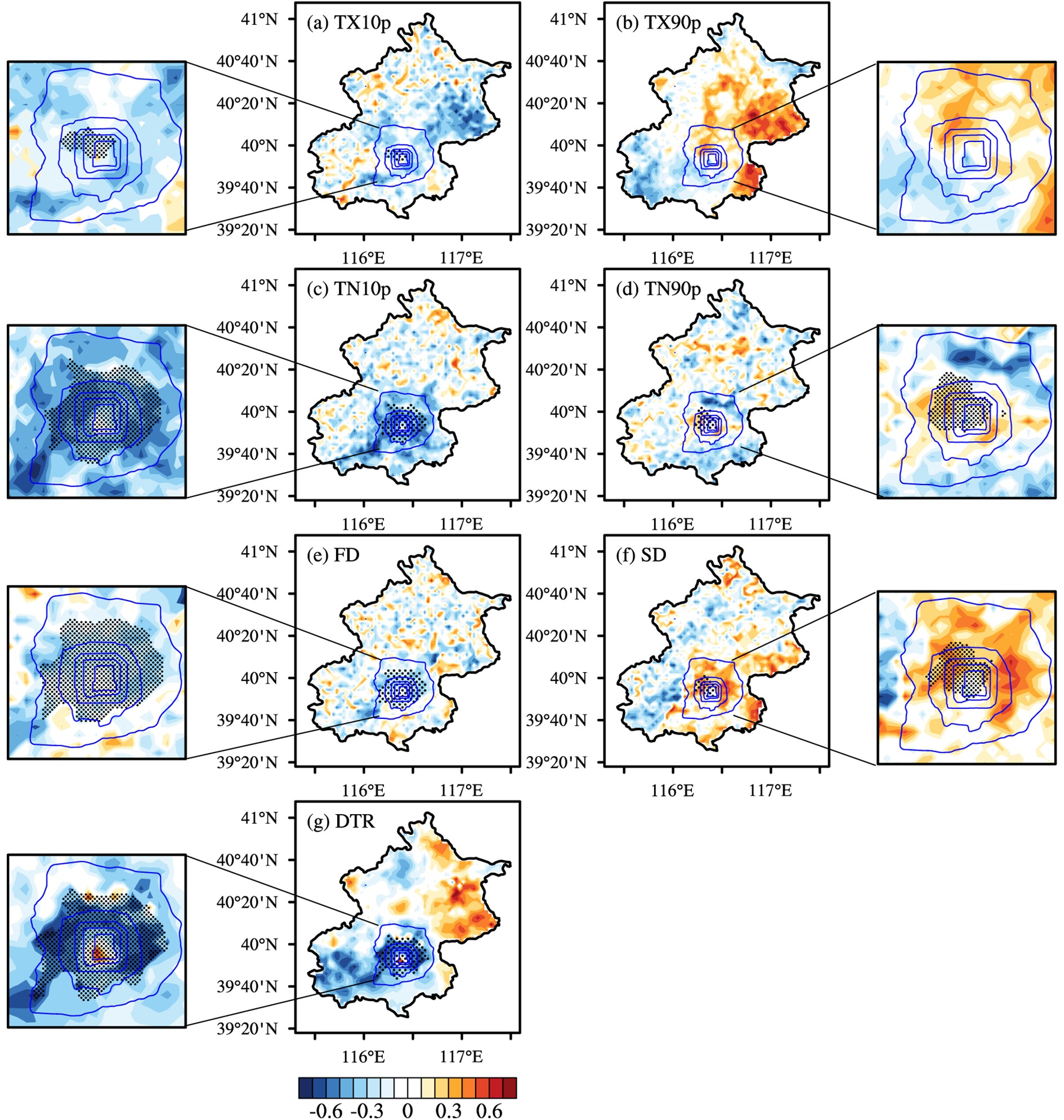Figure9. Spatial distribution of temporal correlation coefficients between AHR and ΔETIs; the ETIs from (a) to (g) represent TX10p, TX90p, TN10p, TN90p, FD, SD and DTR. The shaded areas, which passed the t-test at a confidence level of 90%, indicate that the differences in extreme temperature events were significant when releasing anthropogenic heat flux.



2 -->

4.3. Mechanisms of extreme temperature events with AHR

Increases in AHR had an impact on dynamic processes in the atmospheric boundary layer. The planetary boundary layer height (PBLH) increased with rising AHR (Figs. 10a-c), with this change in PBLH amounting to more than a 100-m increase in the city center. The convergence of 10-m surface wind was also strengthened (Fig. 10g-i), with air converging in the city center and moving to the higher atmosphere, which also strengthens the vertical exchange of energy. Moreover, higher PBLH and stronger winds made the near-surface atmosphere less stable. With stronger vertical transportation, heat transfers from the near-surface to the higher atmosphere are easier, and this will cool the near-surface temperature, which can be called the cooling effect. AHR is one of the biggest influencing factors on urban heat islands, and some researchers have already found a synergistic effect between urban heat islands and heat waves (Li and Bou-Zeid, 2013). Hence, AHR may have a relationship with extreme heat events, when the high temperature reaches some specified level. Some researchers have discovered that enhanced evaporation and lowering of near-surface humidity can lead to more heat convergence, making extreme heat events happen more easily (Freychet et al., 2017). However, in the results of this study, specific humidity had little change and did not pass the t-test at a confidence level of 90% (Figs. 10d-f), showing that AHR influences the extreme temperature events through heating directly.
Figure10. The (a?c) PBLH, (d?f) specific humidity at 2 m (Q2), and (g?i) spatial distribution of the velocity of 10-m (w10) winds, from the (a, d, g) AHR and (b, e, h) no-AHR simulations, and (c, f, i) their differences. The shaded areas passed the t-test at a confidence level of 90%.


Extreme temperature events in this study were found to be controlled by the heating effect of AHR, but can be relieved slightly due to the cooling effect of the boundary layer dynamic process. Here, ?ΔPBLH is used to represent the dynamic process, assuming that the dynamic process strength varies negatively with temperature and positively with PBLH. A multiple regression of ΔETI, AHR, and ?ΔPBLH was performed; all the data were normalized firstly to remove the effect of the order of magnitude. As shown in Table 7, the boundary layer dynamic process depressed the number of occurrences of extreme temperature events and reduced the impact of AHR on these events. Extreme heat events are more frequent with greater AHR, but the boundary dynamic process damps down the tendency toward an increase. For cold extreme events, for example, the regression coefficients of anthropogenic heat for TX10p and TN10p were ?0.081 and ?0.319, and those of vertical transportation were 0.521 and 0.572. Extreme cold events are less frequent with greater AHR, but the boundary layer dynamic process damps down the tendency toward a decrease. Extreme heat events have the opposite tendency, being more frequent with greater AHR. Heating is the main effect of AHR, by increasing sensible heat flux and raising urban temperatures. It shows seasonal variation in heating efficiency with temperature, with winter temperatures increasing more than summer temperatures for each unit of AHR. Multiple linear regression of ΔT, AHR, and ?ΔPBLH was performed in the urban area to reveal the direct heating effect of AHR and the cooling effect of atmospheric dynamic processes in different seasons (shown in Table 8). The regression coefficients of AHR from spring to winter are 0.21, ?0.258, 0.128 and 0.381. The results show that winter has a larger regression coefficient of AHR than the other seasons and that the heating effect of AHR in winter is about 1.6 times stronger than over the whole year for the temperature rise. In addition, the negative regression coefficient in summer reveals that AHR may have an opposite effect to the trend towards a temperature rise. The regression coefficients of ?ΔPBLH from spring to winter are ?0.81, 0.90, ?0.88 and ?0.42. From comparisons of the absolute regression coefficients of ?ΔPBLH over the four seasons, it was concluded that the impact of the boundary layer atmospheric dynamic process on the temperature rise, with the strongest effect in summer and the weakest in winter, is quite opposite to that of AHR. Note also that the absolute regression coefficients of ?ΔPBLH were always larger than those of AHR, which means that ?ΔPBLH is more related to trends in ΔT, but it does not necessarily make a larger contribution than AHR.

	TX10p	TX90p	TN10p	TN90p	FD	SD	DTR
a	?0.081	?0.126	?0.319	0.057	?0.124	0.140	?0.459
b	0.521	?0.528	0.572	?0.583	0.380	?0.553	0.445
c	?1.60×10?7	6.38×10?8	1.46×10?8	4.91×10?8	4.59×10?8	1.15×10?8	1.38×10?7
Notes: a, b and c are multiple regression coefficients in the formula $ \Delta {\rm{ETI}} = a \times {\rm{AHR}} + b \times \left({ - \Delta {\rm{PBLH}}} \right) + c$; $ {\Delta }{\rm{ETI}} $, AHR and $ -{\Delta }{\rm{PBLH}} $ are normalized in the regression process.

Table7. Multiple linear regression of ΔETI, AHR and ?ΔPBLH.

	Year	Spring	Summer	Autumn	Winter
a	0.082	0.210	?0.258	0.128	0.381
b	?0.880	?0.811	?0.896	?0.879	?0.422
c	1.99×10?7	5.37×10?8	?7.75×10?9	?2.85×10?8	?1.27×10?6
Notes: a, b and c are multiple regression coefficients in the formula $\Delta T = a \times {\rm{AHR}} + b \times \left({ - \Delta {\rm{PBLH}}} \right) + c$; ${\Delta }{{T} }$, AHR and $ -{\Delta }{\rm{PBLH}} $ are normalized in the regression process.

Table8. Multiple linear regression of ΔT, AHR and ΔPBLH.

This paper has revealed the relationship between AHR from energy consumption and extreme temperature events in a case study of Beijing, China. Temporal and spatial variation data for AHR were processed, which were based on energy consumption, population density, and previous research. AHR increased to a steady state with declining use of coal and more widespread use of clean energy from 2001 to 2017. AHR is mainly concentrated within the six ring roads of Beijing, with a higher monthly profile in winter. Besides, its spatial variation was much larger than its variation over time. A new AHR scheme incorporating abrupt temperature changes was implemented in the WRF model. Two experiments, with and without AHR, were performed to simulate the effect of AHR on climate in the case study. Temperature rise due to the AHR heating effect was mainly concentrated in the urban center. In spring, summer, fall and winter, the temperature increased by 0.36°C, 0.19°C, 0.62°C and 0.93°C, respectively, with similar seasonal variations in AHR. However, the heating efficiencies were different, with the smallest temperature increase per unit AHR in summer and the largest increase in winter. Both extreme heat events and extreme cold events could be represented using seven extreme temperature event indices. AHR reinforced the occurrence of extreme heat events, but restrained the development of extreme cold events, with an increase in extreme heat events of 0.11 days for warm days (ΔTX90p), 0.02 days for warm nights (ΔTN90p), and 0.19 days for summer days (ΔSD), and an annual decrease in extreme cold events of 0.26 days for cold days (ΔTX10p), 0.56 days for cold nights (ΔTN10p), and 0.39 days for frost days (ΔFD) in the city center. In addition, the diurnal temperature range (ΔDTR) was narrower. It shows that the decrease in the frequency of annual extreme cold events is larger than the increase in the frequency of annual extreme heat events. The reason might be that coal and oil consumption release more anthropogenic heat flux in winter and weaken the effect of vertical transportation, which decreases the frequency of extreme cold events. Besides, the correlation coefficients between AHR and ETI differences (ΔETIs) and the regression coefficients both show the strong signal of this trend in the city center.
Note also that AHR and the atmospheric dynamic process play opposite roles in urban temperature rises and the occurrence of extreme temperature events. The dynamic process restrains the increasing trend in extreme heat events and helps increase the number of extreme cold events. In addition, the effect of lower heating efficiency in summer than in other seasons could be making a contribution, with strong convection transferring heat to the higher atmosphere and reducing the warming ability.
A possible limitation is that ignoring the typical routes taken by inhabitants, as well as the distributions of workplaces and thermal plants, will result in AHR estimation errors. However, larger regional analysis will weaken the influence of the uncertainty of AHR, and that is why we divided Beijing into three parts to analyze the relationships between AHR and extreme temperature events. Also, the results were obtained from a case study, but the study method can still be applied to other cities with different simulation areas. From our research, AHR heated the atmosphere which changed the frequencies and trend of extreme temperature events. According to the global high-resolution anthropogenic heat release data, cities in northern mid-latitudes (such as Dalian, Shanghai, Guangzhou, Taiwan and cities of Yangtze River Delta in East China, Seoul of South Korea, Tokyo of Japan, lots of cities in Europe like Amsterdam, London and Lodz, San Francisco, New York and Washington DC in United States) which release more anthropogenic heat shall have more significant influence than other places on extreme temperature events. Developing countries like China, India and Egypt have a stronger increasing tendency of extreme temperature events due to higher energy consumption growth. However, the results may be changed with different energy management practices, as well as dynamic processes in the atmospheric boundary layer.
Finally, it is foreseeable that decreasing AHR by reducing energy consumption could be a way to mitigate extreme heat events, but might not be helpful in dealing with extreme cold events. For Beijing, it is reasonable to reduce energy consumption to deal with extreme heat events because of hot days in summer; meanwhile, energy consumption could be adjusted to keep the city warm and decrease extreme cold events in winter.
Acknowledgements. This work was supported by the Strategic Priority Research Program of the Chinese Academy of Sciences (Grant No. XDA23090102), the National Natural Science Foundation of China (Grant No. 41830967), the Key Research Program of Frontier Sciences, Chinese Academy of Sciences (Grant No. QYZDY-SSW-DQC012), and the National Key Research and Development Program of China (Grant Nos. 2018YFC1506602 and 2020YFA0608203). We also thank the National Meteorological Information Center, China Meteorological Administration, for data support.