Yuhan LIU¹,
Hongli WANG²,
Shengao JING²,
Ming ZHOU¹,
Shenrong LOU²,
Kun QU¹,
Wanyi QIU¹,
Qian WANG²,
Shule LI¹,
Yaqin GAO²,
Yusi LIU³,
Xiaobing LI⁴,
Zhong-Ren PENG⁵,
Junhui CHEN⁶,
Keding LU^1,,

Corresponding author: Keding LU,k.lu@pku.edu.cn

1.State Key Joint Laboratory of Environment Simulation and Pollution Control, College of Environmental Sciences and Engineering, Peking University, Beijing 100871, China
2.State Environmental Protection Key Laboratory of Formation and Prevention of Urban Air Pollution Complex, Shanghai Academy of Environmental Sciences, Shanghai 200233, China
3.State Key Laboratory of Severe Weather & Key Laboratory for Atmospheric Chemistry of China Meteorology Administration, Chinese Academy of Meteorological Sciences, Beijing 100081, China
4.Guangdong-Hongkong-Macau Joint Laboratory of Collaborative Innovation for Environmental Quality, Institute for Environmental and Climate Research, Jinan University, Guangzhou 510632, China
5.International Center for Adaptation Planning and Design, College of Design, Construction and Planning, University of Florida, Gainesville 32611, FL, USA
6.Sichuan Academy of Environmental Science, Sichuan 610041, China
Manuscript received: 2020-06-20
Manuscript revised: 2020-11-26
Manuscript accepted: 2021-01-07
Abstract:As Volatile Organic Compounds (VOCs) are one of the precursors of ozone, their distribution and variable concentrations are highly related to local ozone pollution control. In this study, we obtained vertical profiles of VOCs in Shanghai’s Jinshan district on 8 September and 9 September in 2016 to investigate their distribution and impact on local atmospheric oxidation in the near surface layer. Vertical samples were collected from heights between 50 m and 400 m by summa canisters using an unmanned aerial vehicle (UAV). Concentrations of VOCs (VOCs refers to the 52 species measured in this study) varied minimally below 200 m, and decreased by 21.2% from 100 m to 400 m. The concentrations of VOCs above 200 m decreased significantly in comparison to those below 200 m. The proportions of alkanes and aromatics increased from 55.2% and 30.5% to 57.3% and 33.0%, respectively. Additionally, the proportion of alkenes decreased from 13.2% to 8.4%. Toluene and m/p-xylene were the key species in the formation of SOA and ozone. Principal component analysis (PCA) revealed that the VOCs measured in this study mainly originated from industrial emissions.
Keywords: VOCs,
vertical profiles,
secondary organic aerosol,
PCA,
Ozone
摘要:挥发性有机物（VOCs）作为环境大气臭氧（O₃）的重要前体物，其在环境大气中的浓度以及分布与O₃的局地化学生成高度相关。本研究在2016年9月8日和9月9日，通过使用无人机搭载VOCs采样罐的形式，对上海市郊区的50米至400米高度的环境大气进行离线采样分析。VOCs廓线的分析结果显示，环境大气中的VOCs浓度在200米高度之下变化幅度较小，从100米高度到400米高度VOCs浓度能够降低21.2%。对不同高度的VOCs组成成分分析发现，烷烃和芳香烃的占比分别从55.2%和30.5%上升至57.3%和33.0%。但是烯烃的占比却从13.2%下降到8.4%。在对环境大气中不同高度下的VOCs的O₃生成潜势（OFP）和二次有机气溶胶（SOA）生成潜势（SOAFP）进行计算发现，苯、间/对-二甲苯是对当地O₃和SOA生成贡献最大的关键物种。在使用主成分分析（PCA）方法对当地VOCs来源进行解析发现，当地VOCs主要来自于工业排放。
关键词:VOCs,
垂直廓线,
二次有机气溶胶,
PCA,
臭氧

HTML

--> --> -->

Volatile Organic Compounds (VOCs) are key constituents in tropospheric chemistry and are the major precursors of tropospheric ozone and secondary organic aerosols (SOA), which are known play a key role in atmospheric air quality and the ecological environment (Jerrett et al., 2009; Cooper et al., 2010). VOCs play an important role in tropospheric chemical processes, as they can react with NO_x in the presence of solar radiation to form ozone. VOCs can also react with OH radicals, O_3, and NO₃ as gaseous precursors to form secondary organic aerosols (SOA). The lifetimes of VOCs in the atmosphere are controlled by their rate constants of VOCs with these oxidants, which can span across several orders of magnitude (Parrish et al., 2007).
In recent years, air pollution events have occurred more frequently in China as a result of rapid economic development. This phenomenon has attracted both public and research attention. Although particle pollution has been of the greatest concern, the control of ozone pollution is also urgent. Field studies in northern China have shown that summertime ozone concentrations increased by 2 ppbv yr^–1, from 2003 to 2015, despite reduced NO_x emissions (Sun et al., 2016). Extremely high ozone concentrations (> 200 ppbv) have also been frequently reported (Zhang et al., 2007, 2008; Xue et al., 2016), and regional ozone pollution has even occurred in the non-economically developed areas of western China (Tan et al., 2018). The Yangtze River Delta (YRD) is one of the three most developed regions in China and faces serious ozone pollution as a result of the rapid urbanization and industrialization that has taken place in recent years (Huang et al., 2011; Li et al., 2017; She et al., 2017). Due to the facts that VOCs are the key precursor of ozone formation and that previous studies have pointed out that ozone formation in the YRD is largely dependent on VOCs (Geng et al., 2009; Jin and Holloway, 2015), a full understanding of tropospheric VOCs in this area could assist in the development of more rational ozone control strategies.
Most field measurements of VOCs have focused upon the concentrations and composition of ground-level VOCs (Yuan et al., 2013; Cheng et al., 2016; An et al., 2017; Liu et al., 2018; Sheng et al., 2018; Wang et al., 2018). To truly understand the formation of ozone and secondary organic aerosol in the planetary boundary layer, especially the lowest few hundred meters, research on vertical profiles of VOCs becomes necessary. The study of vertical profiles of VOCs, in the troposphere, can help us better understand their concentration, distribution, and chemical changes which occur at different heights, thus deepening the understanding of their effects on ozone and secondary organic aerosol formation in the vertical direction. The most used techniques for studying vertical profiles are aircraft (Borbon et al., 2013), tethered balloons (Glaser et al., 2003; Sangiorgi et al., 2011; Tsai et al., 2012; Zhang et al., 2018), and towers (Lin et al., 2011; Mao et al., 2008; Zhang et al., 2020). Tethered balloons can sample up to a height of 1000 m (Sun et al., 2018; Wu et al., 2020), but require large space and only operate for short-flight distances. Tower-based sampling techniques are limited by the height and location of the tower. The maximum height of air samples successfully gathered by this technique was about 280 m (Mao et al., 2008). Aircraft techniques could overcome the limit of sampling heights and locations, and could be used to collect samples up to 12 km in height, but the interference from fuel-powered engines and the danger of low-altitude flight (lower than 500 m) limit the application and practicality of this technique in the context of near-surface, atmospheric research. Unmanned aerial vehicles (UAVs) have become a new option for vertical profile studies in recent years. Compared to the aforementioned techniques, UAVs are able to hover and require a small space for landing (Klemas, 2015). For the study of the vertical profiles of VOCs, UAVs can be equipped with stainless steel canisters to perform VOCs collection in ambient air (Vo et al., 2018), without the need for a tower, and can also flexibly hover at any height to obtain measurements.
In this work, vertical profiles of VOCs were explored by using a UAV equipped with stainless steel canisters on 8 and 9 September 2016 in the Shanghai’s Jinshan district, eastern China. This is the first attempt to use a UAV to collect air samples in the vertical direction over the Yangtze River Delta. We expect to achieve the following objectives: (1) describe the vertical distribution of VOCs and their evolutionary characteristics; (2) explore the consumed VOCs through transportation; (3) analyze the key species of VOCs in ozone and secondary organic aerosol formation during transportation, and; (4) discuss the source of VOCs in this area.

2

-->

2.1. Sampling

The sampling site is located in Langxia (LX), which is a suburban site in Shanghai’s Jinshan district (30°79′N, 121°19′E, Fig. 1). There are two major industrial plants (SIZ—Shanghai Jinshan Second Industrial Zone and JPZ—Jinshan Petrochemical Zone) located 10 km to the southeast of the sampling site, which are the two major sources of VOC emission in Jinshan district. The SIZ contains a large number of industries, such as electronic information engineering, machinery manufacturing, biomedicine, iron and steel plants, synthetic/new materials, cement, new energy, and research and development technology (Qiu et al., 2019). The JPZ produces aviation kerosene, gasoline diesel, aromatic olefines, and emits VOCs via oil refineries, leakage of storage tanks, and water treatment processes (Kalabokas et al., 2001; Qiu et al., 2019). Five air sampling flights were conducted over this sampling site at 1000?1200 LST 8 and 9 September 2016, and 1400?1600 LST on 8 September 2016, and 0900?1000, 1300?1500, 1600?1800 LST on 9 September 2016. Five targeting heights of 50 m, 100 m, 200 m, 300 m and 400 m were obtained in all five sampling flights. All samples were transferred to the State Environmental Protection Key Laboratory of Urban Air Pollution Complex at Shanghai Academy of Environmental Sciences for the analysis of VOCs. An on-line monitoring station for VOCs was set up at Xinlian (XL), which is located on the northwest border of the SIZ.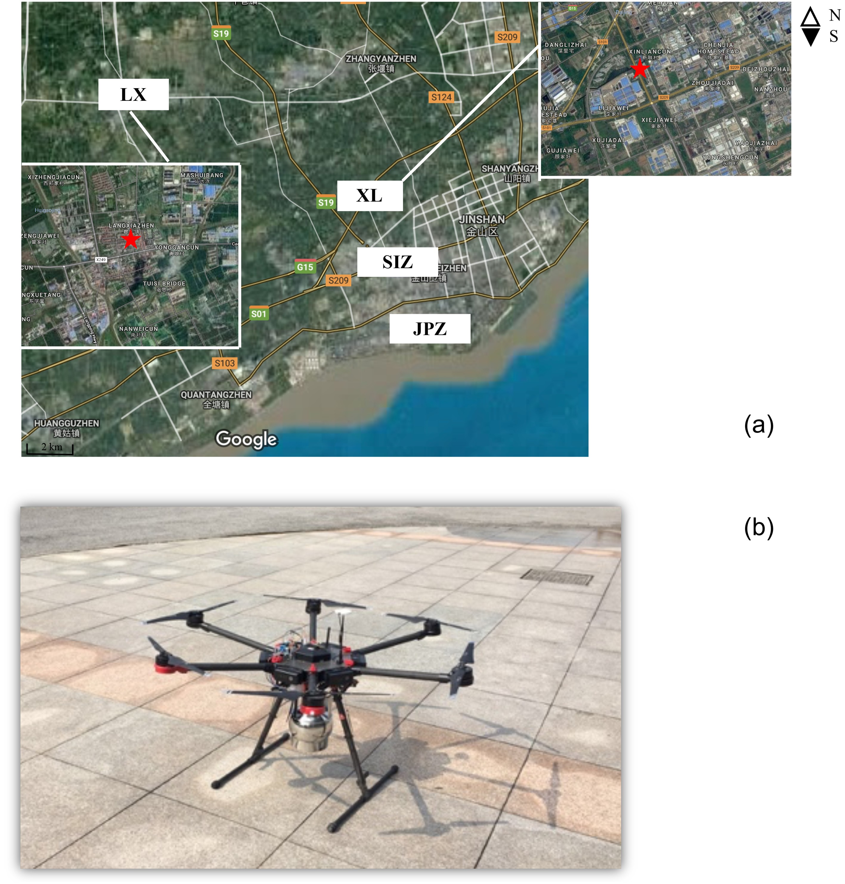
Figure1. (a) Locations of observation sites of Langxia (LX) and Xinlian (XL), and (b) unmanned aerial vehicle (UAV) used for volatile organic compounds (VOCs) sampling.


The collection of samples for analysis of VOCs was carried out by a UAV (M600, DJI, China, Fig. 1), which included a remote-controlled 3.2 L canister that was attached to the lower part of the UAV. The UAV had eight wings and was equipped with a power motor (DJI 6010) and six 4500 mAh LiPo 6s batteries (capable of sustaining flight and hovering for 30 minutes). The maximum loaded weight was 15 kg. To avoid interference with VOCs, the canister inlet was 20 cm above the UAV border. The UAV, equipped with the canister, travelled vertically at 2 m s^–1, and hovered for one minute while sampling at each targeting height during each flight. Vertical profiles of temperature and relative humidity were obtained from a L-band sounding system which was acquired from the China Meteorological Administration (http://data.cma.cn/).

2 -->

2.2. VOCs analysis.

The concentrations and compositions of 52 VOCs [Table S1 in the electronic supplementary material (ESM)] captured in the sampling canisters were analyzed using a gas chromatography-mass spectrometry instrument (GC-MS, Agilent, GC model 7820A, MSD model 5977E). Briefly, a 500 mL full-air sample was taken from the sampling canister and concentrated by a three-stage, cryo-focusing, pre-concentration system (Entech Instruments, Inc., USA). The vaporized VOCs were then injected into the gas chromatography system by a helium carrier gas for analysis. A PLOT (Al₂O₃ KCl^–1) column (15 m, 0.32 mm ID) connected to a flame ionization detector was used to quantify C2-C5 hydrocarbons, and a DB-624 column (30 m, 0.25 mm ID) connected to a mass spectrometer was used to analyze other VOCs species. The carrier for both columns was ultra-pure helium (> 99.999 %). Detailed information is described in Liu et al. (2008) and Wang et al. (2018).

2 -->

2.3. Quality assurance and quality control

The summa canisters (3.2 L each) were cleaned and evacuated (< 10 Pa) prior to sampling. One clean summa canister was selected for analysis of high-purity nitrogen to verify that the canisters were clean. Each canister was connected to a Teflon filter to remove particulate matter and moisture during sampling. The pressure of the canister was re-checked after each flight to ensure it was at 0 Torr. A commercial standard gas containing PAMs (29 alkanes, 11 alkenes, 16 aromatics) was used to identify compounds and confirm their retention times. The response of the instrument for the analysis of VOCs was calibrated after every eight samples using a 1 ppbv PAMs standard gas.

2 -->

2.4. Principal component analysis

Principal component analysis (PCA) has often been used to identify and quantify the major sources of VOCs (Bruno et al., 2001; Duan et al., 2008; Jia et al., 2016). In this study, PCA was used to determine the major source of VOCs in the study area. Statistical analysis was carried out using IBM SPSS Statistics 19 software. PCA was applied to the source profiles and source strengths in absolute VOCs concentrations measured at different heights. Twenty-four VOCs were used for the PCA calculation as they accounted for 65% of the total VOCs at LX. The varimax rotation of the matrix was used in this study to minimize the number of VOCs with high loadings on a factor. Only principal components whose eigenvalues were >1 were retained as a factor. More details regarding the method of PCA can be found in previous studies (Guo et al., 2004, 2007).

2 -->

2.5. Ozone formation potential

VOCs react with OH radicals, which efficiently convert NO to NO₂ and result in the accumulation of ozone. However, individual VOCs can differ significantly in their effects on ozone formation. The ozone formation potential (OFP) is calculated following Eq. (1), which is used to represent the ozone formation probability of individual VOCs.
The index i represents the concentration of a particular species of the VOCs (ppbv) and MIR represents the maximum incremental reactivity of that specie. (Carter et al., 1995).

2

-->

3.1. VOCs vertical profile

Figure 2 presents the results of the average concentrations and compositions of VOCs at different heights in LX. The vertical profiles obtained in this study showed that concentrations increased at elevated heights, and reached a maximum at 100 m (36.1 ppbv) before decreasing continuously. Concentrations of the 52 VOCs measured in this study, at different heights, are listed in Table S1 in the ESM. Concentrations of VOCs (VOCs refers to the 52 species measured in this study) varied less below 200 m, and decreased by 21.2% from 100 m to 400 m. The concentrations of VOCs above 200 m were much lower compared to those below 200 m. Alkanes decreased by 17.3% from 100 m to 400 m. Alkenes and aromatics decreased by 43.0% and 20.5%, respectively, from 200 m to 400 m. Furthermore, we analyzed the average proportion of alkanes, alkenes, and aromatics in VOCs at different heights on 8 and 9 September 2016. The proportion of hydrocarbons did not appear to vary significantly between 50 m and 400 m. The major components of VOCs were alkanes (> 50 %) below 400 m, followed by aromatics (> 30 %).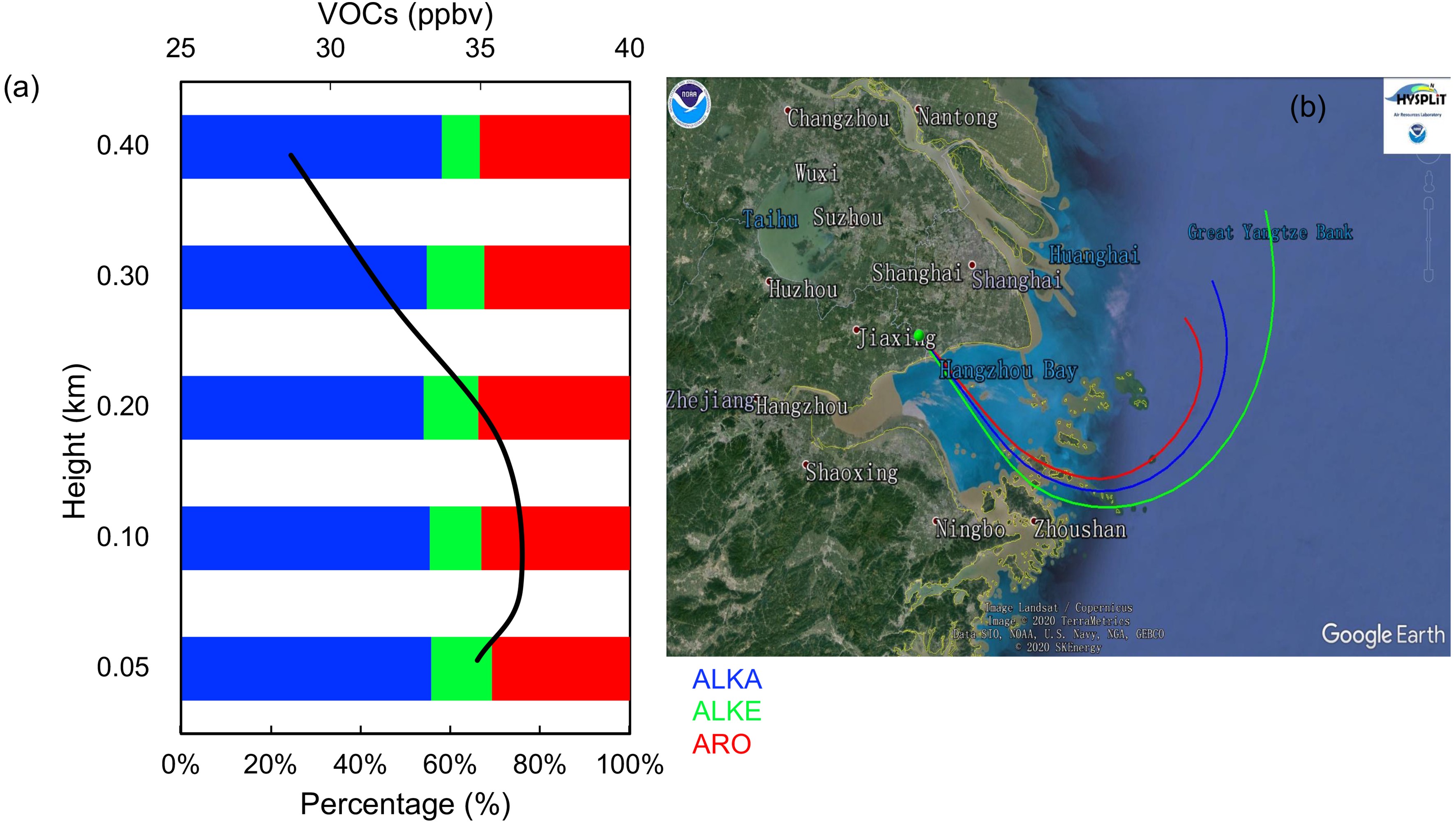
Figure2. (a) Overview of the vertical profile of 52 VOCs measured at Langxia (LX); (b) 24 hours backward trajectory in 3 heights (50 m, 100 m, 200 m) of Langxia (LX) on 9 September 2016 with 1° resolution GDAS data.


By combining the conditions of the sampling site and surrounding areas, we inferred that air masses obtained at the sampling site were transported in from elsewhere. By applying a backward trajectory analysis [Hysplit4 (https://ready.arl.noaa.gov/HYSPLIT.php, Fig. 2b)], we found that the air masses below 500 m were transported from a southeast direction during the sampling period. The SIZ and JPZ industrial plants are located to the southeast of the sampling site; hence, it was further inferred that the air mass at the sampling site during the sampling period may have been transported from these industrial plants. Results of the proportion analysis of VOCs measured at Xinlian (XL) on the northwest border of the SIZ demonstrated that the most abundant hydrocarbons were alkanes (44%) and aromatics (43%) (Fig. S1 in the ESM). The lifetime of most species of alkanes were longer than those of alkenes and aromatics. The concentrations of alkenes and aromatics were therefore consumed during transportation. The proportion of alkanes at LX (a receiver site) was much larger than the proportion of alkenes and aromatics in comparison to those at XL (an emission site). In addition, VOCs had very different lifetimes in the atmosphere, 24 hours of backward trajectory analysis with GDAS (Fig. 2b) gave a rough estimate of the trajectory of air mass movement. Description of this small-scale transportation within GDAS still has its limitations, especially in the judgment of combining VOCs transportation.
By combining the vertical profiles of meteorological variables, the vertical profiles of VOCs concentrations showed two patterns. Figure 3 shows the results from 1000 to 1200 LST on 8 September and the results from 0900 to 1100 LST on 9 September. The concentrations of VOCs increased from the surface (50 m), reaching a maximum value at 200 m (40.4 ppbv) 8 on September and reaching a maximum value at 100 m (60.9 ppbv) on 9 September. Alkanes accounted for more than 50% of the total VOCs at each height. Analysis of the vertical profiles of temperature and relative humidity on 8 September, show that there was an inversion layer at 200 m, which traps the air masses, restricting their vertical movement, resulting in the accumulation of VOCs at 200 m. A similar change also appeared in the vertical profile on 9 September from 0900 to 1100 LST. Figure 4 shows the results from 1400 to 1600 LST on 8 September and the results from both 1300 to 1500 LST and from 1600 to 1800 LST on 9 September. These profiles were taken while the boundary layer was in a strong convective state. The concentration of VOCs decreased slowly with height, with the highest concentration at 50 m (41.8 ppbv on 8 September, 31.4 ppbv and 30.1 ppbv on 9 September) and the lowest concentration at 400 m (30.7 ppbv on 8 September and 19.9 ppbv on 9 September). In the profile from 1300 to 1500 LST on September 9, the minimum value of VOCs concentrations was located at 300 m (17.9 ppbv), and then increased slowly. It may be caused by long-distance transportation from the SIZ. Alkanes were the dominant component of VOCs at each height.
Figure3. Vertical profiles of the VOCs concentration and meteorological variables (temperature and relative humidity). (a) Vertical profile of VOCs concentrations during 1000?1200 LST on 8 September 2016, vertical profile of temperature and relative humidity at 0700 LST on 8 September; (b) Vertical profile of VOCs concentrations during 0900?1100 LST on 9 September 2016, vertical profile of temperature and relative humidity at 0700 LST on 9 September.


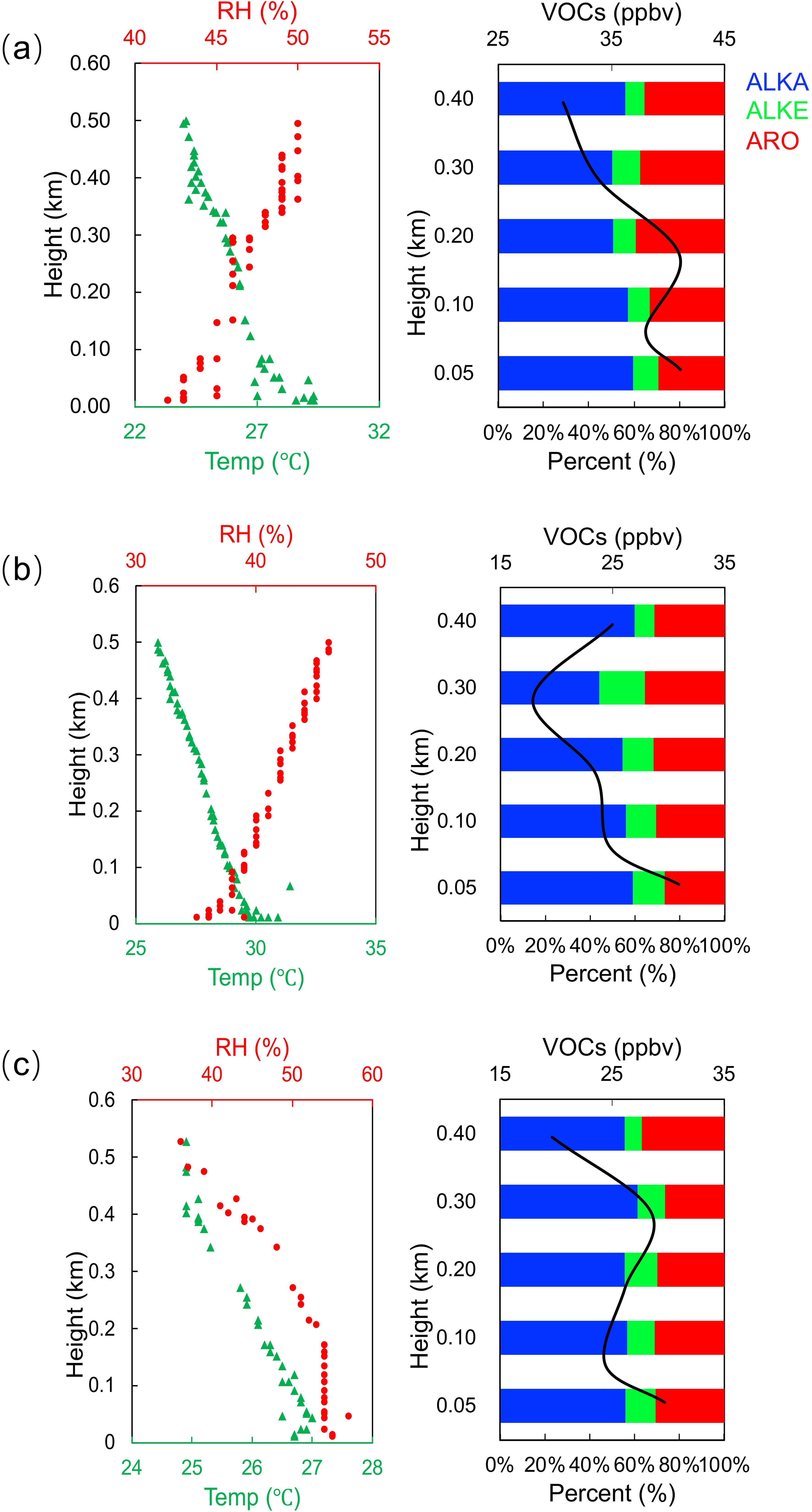Figure4. Vertical profiles of the VOCs concentration and meteorological variables (temperature and relative humidity). (a) Vertical profile of VOCs concentrations during 1400?1600 LST on 8 September 2016, vertical profile of temperature and relative humidity at 1300 LST on 8 September; (b) Vertical profile of VOCs concentrations during 1300?1500 LST on 9 September 2016, vertical profile of temperature and relative humidity at 1300 LST on 9 September; (c) Vertical profile of VOCs concentrations during 1600?1800 LST on 9 September, vertical profile of temperature and relative humidity at 1900 LST on 9 September.



2 -->

3.2. Contribution of VOCs oxidants to SOA formation and ozone formation

The consumption of VOCs during transportation from XL to LX may have generated ozone and promoted the formation of SOA. In this section, we discuss the effects of the VOCs consumed during transportation by atmospheric oxidation. The loss of VOCs in the atmosphere depends on the photochemical age, which is defined as the time integrated exposure to OH radicals. A simple dilution chemistry model can be used to describe the changes of VOCs concentrations over the time. Twelve VOCs species with different OH reactivities were selected to calculate the OH exposure during the transportation process from XL to LX. Their concentrations at LX are given by Eq. (2):
where $ C_{t\left(i\right)} $ is the concentration of ith species at LX, D(t) is a dilution factor, $ C_{{0(}i{)}} $ is the initial concentration of the ith species, $ k_{{\rm{OH}},i} $ is the reaction rate constant of the ith specie with OH radicals, and $ {({\rm{OH}})\Delta t}$ is time of exposure to OH radicals. The dilution factor and time of exposure to OH radicals can be obtained from Eq. (3)?Eq. (4):
Species i and j were selected from 12 VOCs species that covered a wide range of OH reactivities from $ {\rm{2}}{\rm{.3 \times 1}}{{\rm{0}}^{{\rm{ - 12}}}}\;{\rm{c}}{{\rm{m}}^{\rm{3}}}\;{\rm{molecul}}{{\rm{e}}^{{\rm{ - 1}}}}\;{{\rm{s}}^{{\rm{ - 1}}}}$ (n-butane) to ${\rm{3 \times 1}}{{\rm{0}}^{{\rm{ - 11}}}}\;{\rm{c}}{{\rm{m}}^{\rm{3}}}$$\;{\rm{molecul}}{{\rm{e}}^{{\rm{ - 1}}}}\;{{\rm{s}}^{{\rm{ - 1}}}}$ (propene). The initial concentrations reflected the observed nocturnal data because we thought that VOCs mainly originated from direct emissions during the night. More than one pair of VOCs were considered in this study, we used sets of VOCs measurements (m/p-xylene, o-xylene, benzene, toluene, cyclohexane, n-pentane, n-butane, i-pentane, i-butane, ethylbenzene, propane, and propene) in a single age determination by performing a linear regression of $ \ln \left[{C}_{t\left(i\right)}/{C}_{0\left(i\right)}\right] $ versus k_i. The $ \left[ {{\rm{OH}}} \right]\Delta {{t}} $ results at different heights at the LX site are shown in Fig. S2 in the ESM, whereby the average OH exposure ranged from $ {\rm{8}}{\rm{.01 \times 1}}{{\rm{0}}^{{\rm{10}}}}$ to ${\rm{11}}{\rm{.47 \times 1}}{{\rm{0}}^{{\rm{10}}}}\;{\rm{molecules}}\;{\rm{c}}{{\rm{m}}^{{\rm{ - 3}}}}\;{\rm{s}}$. It was inferred from the distribution of $ \left[ {{\rm{OH}}} \right]\Delta {{t}}$ that OH radicals were relatively uniform below 400 m, thus indicating that the atmosphere was well-mixed at the observed height, and the atmospheric oxidation observed at different heights were similar. By varying the $ \left[ {{\rm{OH}}} \right]\Delta {{t}} $ at different heights and the initial VOCs concentrations, we calculated the consumed VOCs (C_i,consumed) during the transportation using Eq. (5):
Here, C₀ is the initial concentration of the VOC in question (ppbv) that was measured at the XL site, D is a dilution factor, k_OH,i is the reaction rate constant of the particular VOC with OH radicals, and $ ( {{\rm{OH}}} )\Delta {{t}} $ is the time of exposure to the OH radicals. Through photochemical reactions, VOCs are able to generate SOA during the oxidation process; hence, the secondary organic aerosol formation potential (SOAFP) demonstrates the ability to generate SOA via the oxidation of VOCs. Most previous studies on the topic have focused on SOAFP calculations at the observed site, and ignored the impact of consumed VOCs during transportation upon SOA formation. Within the consumed VOCs concentrations and the SOA yields (Grosjean and Seinfeld, 1989; Wu et al., 2017), we obtained the SOAFP of consumed VOCs during transportation using Eq. (6):
Here $ {\rm{SOAFP}}_{i} $ is the SOAFP for species i, $ C_{i, \;{\rm{consumed}}} $ is the consumed i via transportation, and $ {{Y}}_{i} $ is the SOA yield for species i, from literature references (Wu et al., 2017). We obtained the SOAFP of consumed VOCs on 8 and 9 September 2016, from heights of 50 m to 400 m (Table 1). The SOAFP ranged from 19.7 $ {\rm{\mu g}}\;{\rm{c}}{{\rm{m}}^{\rm{3}}} $ to 22.5 $ {\rm{\mu g}}\;{\rm{c}}{{\rm{m}}^{\rm{3}}} $ on 8 September, when the major contributors were toluene, m/p-xylene and o-xylene. On 9 September, the SOAFP exhibited no significant variation in the trend between 50 m and 400 m, but these values were much lower than those on 8 September. The SOAFP results for the vertical profile demonstrated that regardless of whether it was the high value on 8 September or the low value on 9 September, the air mass below 400 m was well-mixed as the SOAFP showed no large fluctuations. The key species of controlling the formation of SOA was toluene and o-xylene.

Height (m)	8 Sep.					9 Sep.
	SOAFP (μg cm?3)	Top 3 species and its proportion of SOAFP	OFP (ppb)	Top 3 species and its proportion of OFP		SOAFP (μg cm?3)	Top 3 species and its proportion of SOAFP	OFP (ppb)	Top 3 species and its proportion of OFP
50	21.2	toluene ($ {\rm{52}}{\rm{.4\% \pm 0}}{\rm{.5\% }}$) m/p-xylene ($ 15.3\% \pm 0.4\% $) o-xylene ($ 11.2\% \pm 0.2\% $)	469	propene ($ 26.1\% \pm 0.4\% $) ethene ($ 20.6\% \pm 0.2\% $) m/p-xylene ($ 20.4\% \pm 0.2\% $)		9.1	toluene ($ 72.1\% \pm 0.1\% $) cyclohexane ($ 8.8\% \pm 0.0\% $) o-xylene ($ 5.2\% \pm 0.0\% $)	112	ethene ($ 21.3\% \pm 1.3\% $) Propene ($ 17.4\% \pm 1.0\% $) Toluene ($ 16.5\% \pm 1.0\% $)
100	22.5		471			9.1		112
200	19.7		445			9.4		114
300	21.0		466			9.2		113
400	21.9		478			9.5		100

Table1. Values of secondary organic aerosol formation potential (SOAFP) and ozone formation potential (OFP) of total VOCs during transportation at Langxia (LX) from heights of 50 m to 400 m and the top three volatile organic compounds (VOCs) species with the highest proportion of SOAFP and OFP on 8 and 9 September 2016


We also analyzed the impact of consumed VOCs to ozone formation during transportation. The analysis (Table 1) showed that the major VOCs species in the OFP calculation were propene ($ {26.1\% \pm 0.4\%} $), ethylene ($ {20.6\% \pm 0.2\%} $), and m/p-xylene ($ {20.4\% \pm 0.2\%} $) on 8 September 2016, whereas those on 9 September 2016, were ethylene ($ {21.3\% \pm 1.3\%} $), propene ($ {17.4\% \pm 1\%} $), and toluene (16.5% $ {\pm } $ 1$ {\%} $). The OFP values on 8 September were four times larger than those on 9 September regardless of the sampling height, thus indicating that the OFP on 8 September was much higher than that on 9 September. This may have been caused by different concentrations of VOCs and other species on these two days. Considering the impact of consumed VOCs during transportation on SOA formation and ozone formation, it was found that toluene and m/p-xylene are the key species for both SOA and ozone formation in the near-surface layer at the sampling site.

2 -->

3.3. Sources apportionment of VOCs using PCA

Twenty-four compounds out of the 52 VOCs measured at the LX site were selected for the PCA as they were the most abundant compounds. Kaiser’s criteria were adopted to determine the appropriate number of factors to be retained (only factors with eigenvalues > 1).
Six factors were extracted from the application of the PCA to the vertical data (Table 2). The first factor explained 64.06 % of the total variance. High loadings were found on propene, 1-butene, hexane, benzene, and cyclohexane. C3?C4 alkenes were associated with combustion. Hexane and cyclohexane mainly came from an oil refinery or chemical plant that is related to the petrochemical industry. Benzene may have come from painting, combustion, or a chemical plant. When combined with other high loadings in factor 1, we assumed that benzene came from a chemical plant. Factor 1 featured the source of the VOCs from the petrochemical industry. The second factor explained 9.97 % of the total variance, whereby i-butane, butane, and propane showed the highest factor loading. Given that i-butane, butane, and propane are the characteristic products of LPG (liquefied petroleum gas) (Liu et al., 2008), we related the second factor to LPG. The third factor explained 6.26% of the total variance, and was highly loaded with m/p-xylene, o-xylene, and 2-methylhexane. The former two could have come from painting or vehicle emission, however, as 2-methylhexane is a tracer of gasoline evaporation (Liu et al., 2008), we determined that factor 3 was probably related to vehicle emissions. The fourth factor explained 4.74% of the total variance, and was highly loaded on 1,3,5-trimethylbenzene and 1,2,4-trimethylbenzene, which are directly emitted to the atmosphere from motor vehicle exhaust and the evaporation of solvents (Luo et al., 2019). The fifth factor explained 4.13% of the total variance, and was highly loaded on styrene, which we related to being sourced from the chemical plant. The sixth factor explained 3.56 % of the total variance, and was highly loaded on dodecane. As dodecane is mainly directly emitted from diesel vehicles, we determined that factor 6 was related to diesel vehicles emission.

VOCs species	1	2	3	4	5	6
ethane	0.64	0.17	?0.07	?0.34	0.07	0.04
propene	0.93	0.20	0.22	0.02	0.02	0.00
propane	0.32	0.82	0.34	0.13	0.02	0.04
i-butane	0.34	0.86	0.24	0.09	?0.03	0.07
1-butene	0.88	0.30	0.29	0.13	0.08	?0.02
butane	0.52	0.78	0.26	0.16	0.08	0.07
i-pentane	0.36	0.65	0.13	0.32	0.34	?0.01
n-pentane	0.67	0.58	0.31	0.14	0.18	0.09
cyclopentane	0.59	0.59	0.27	0.20	0.31	?0.06
2-methylpentane	0.77	0.44	0.23	0.14	0.25	?0.08
3-methylpentane	0.67	0.64	0.26	0.12	0.16	?0.03
hexane	0.83	0.38	0.29	0.10	0.09	?0.01
methylcyclopentane	0.71	0.43	0.48	0.14	0.13	?0.02
Benzene	0.90	0.29	0.25	0.04	0.02	?0.02
cyclohexane	0.83	0.25	0.46	0.05	0.00	0.01
2-methyl-hexane	0.10	0.42	0.73	0.12	0.36	0.13
toluene	0.37	0.72	0.52	0.09	0.12	0.11
ethylbenzene	0.61	0.42	0.65	0.08	0.00	0.02
m/p-xylene	0.45	0.24	0.84	0.06	0.02	0.02
styrene	0.12	0.11	0.10	0.11	0.94	0.03
o-xylene	0.37	0.29	0.85	0.08	0.03	0.05
dodecane	?0.04	0.08	0.09	0.01	0.03	0.99
1,3,5-trimethylbenzene	0.03	0.18	0.03	0.96	0.07	0.01
1,2,4-trimethylbenzene	0.06	0.17	0.12	0.95	0.09	0.01

Table2. Rotated component matrix of 24 volatile organic compounds (VOCs) from 50 m to 400 m


Overall these six factors explained 92.71% of the total variance and could be classified according to the following source categories: 1) petrochemical industry, 2) LPG, 3) vehicle emission. As factor 4 was related to motor vehicle emission and factor 6 was related to diesel vehicle emission, we combined these with factor 3 as vehicle emission sources. As factor 5 was highly related to a chemical plant, this was combined with factor 1 as a petrochemical industry source.

In this study, we conducted vertical atmospheric measurements of VOCs in Shanghai’s Jinshan district using a UAV on 8 and 9 September 2016. Vertical samples were collected from heights of between 50 m and 400 m by summa canisters using an unmanned aerial vehicle (UAV). The proportions of alkanes and aromatics increased from 55.2% and 30.5% to 57.3% and 33.0%, respectively, and the proportion of alkenes decreased from 13.2% to 8.4%. We focused on the impact of consumed VOCs on the ozone formation and SOA formation during transportation and found that toluene and m/p-xylene were the key species for ozone and SOA formation in the study area and that the major source of VOCs was the petrochemical industry.
In this study, we did a preliminary study on the distribution and impact of VOCs upon atmospheric oxidation below 400 m. However, the distribution of VOCs and their effect on oxidative properties of the troposphere are still worthy of further research.
Acknowledgements. This work was supported by the National Natural Science Foundation of China (Grant Nos. 41830106, 21607104), the National Key Research and Development Plan (Grant Nos. 2017YFC0210004, 2018YFC0213801), the Shanghai Science and Technology Commission of Shanghai Municipality (18QA 403600), and the Shanghai Environmental Protection Bureau (2017-2). The author gratefully thanks the science team of Peking University, as well as the team from Jinshan Environmental Monitor Station for their general support. The authors gratefully acknowledge the NOAA Air Resources Laboratory (ARL) for the provision of the HYSPLIT transport and dispersion model and/or READY website (https://www.ready.noaa.gov) used in this publication.
Electronic supplementary material: Supplementary material is available in the online version of this article at https://doi.org/10.1007/s00376-021-0126-y.