HTML
--> --> -->CEFs play a crucial role in modulating interhemispheric moisture transport and the resultant monsoon rainfall. For example, the Somali jet transports a huge amount of water vapor from the Southern Hemisphere and contributes to the Indian monsoon rainfall and the East Asian summer rainfall (Ramesh Kumar et al., 1999; Halpern and Woiceshyn, 2001; Wang and Xue, 2003). In particular, MC-CEF, as the vital water vapor source to East Asia (Wang and Li, 1982; Han, 2002; Zhu, 2012), is regarded as a significant factor contributing to the climate variability in the western North Pacific and East Asia, including the western North Pacific subtropical high (Gao and Xue, 2006; Liu et al., 2009), the activity of tropical cyclones (Han, 2002; Zhao et al., 2012; Feng et al., 2017), and the western North Pacific monsoon trough (Lin et al., 2014).
CEFs are not limited to the lower levels (Xu et al., 1992; Zeng and Li, 2002; Gao and Xue, 2006; Shi et al., 2007; Zhu, 2012), though the lower-level CEFs are the main objective of research. While southerlies prevail in the lower levels in boreal summer, northerlies prevail in the upper levels. The strongest northerlies appear at about 150 hPa, while the strongest southerlies locate at 925 hPa for the MC-CEF and at 850 hPa for the Somali jet. However, the CEFs in the upper levels, especially their variability, have been basically ignored in previous studies. There are only a few previous studies on the vertical structure of the variability in the Somali jet (Qiu and Sun, 2013; Qiu et al., 2014), but these studies focused on the vertical scope below 600 hPa. Integrated analyses of both the lower- and upper-level CEFs are necessary and should prove helpful for a better understanding of CEF variability, particularly if there is a close relationship between the lower- and upper-level CEFs.
It has been well documented that ENSO is the main driver behind the interannual variability of the lower-level MC-CEF and Somali jet. Corresponding to warmer sea surface temperature (SST) in the equatorial central and eastern Pacific, the MC-CEF tends to be strengthened, while the Somali jet weakens (Xu et al., 1992; Wang et al., 2001; Chen et al., 2005), and thus ENSO plays a significant role in the seesaw pattern between the MC-CEF and the Somali jet (Li and Li, 2014; Li et al., 2017a, b). However, whether the variability of the upper-level CEFs is related to ENSO remains unknown.
In this study, we focus on the interannual variability in the CEFs over the Maritime Continent and Indian Ocean, though the CEFs over other regions also have remarkable impacts on climate, such as those over the eastern Pacific affecting ENSO (Wu et al., 2018; Hu and Fedorov, 2018). We also briefly discuss the decadal changes in CEFs, emphasizing the discrepancies among them in different reanalysis datasets. After a description of the datasets and methods in section 2, we evaluate the climatological vertical structure of CEFs and their variability based on three reanalysis datasets in section 3. Section 4 presents the relationship between upper- and lower-level CEFs on the interannual timescale. Lastly, a summary is presented in section 5.
In this study, a 9-yr Gaussian filter is applied to separate the decadal and interannual components. In addition, we perform empirical orthogonal function (EOF) analysis on the meridional winds in a zonal and vertical section along the equator to obtain the leading mode of the CEFs’ variability. For the EOF analysis, data on each grid are mass weighted, following Thompson and Wallace (2000) and Luo and Zhang (2015), i.e., multiplied by the square root of the pressure interval.
In order to quantitatively estimate the relationship between lower- and upper-level CEFs on the interannual time scale, we define several indexes based on the standardized JJA-mean meridional wind anomalies along the equator averaged over specified longitudinal scopes as follows:
● Index for the high-level CEFs over the Maritime Continent (MC-HCEFI): 200 hPa, 110°?170°E;
● Index for the high-level CEFs over the Indian Ocean (IO-HCEFI): 150 hPa, 45°?75°E;
● Index for lower-level CEFs over the Maritime Continent (MC-LCEFI): 925 hPa, 102.5°?110°E, 122.5°?130°E, 147.5°?152.5°E;
● Index for the Somali jet (Somali-I): 850 hPa, 37.5°?62.5°E.
The reasons for these pressure levels and longitudinal scopes are given in section 4.
 Figure1. Climatology of the JJA-mean meridional winds along the equator based on (a) ERA-Interim, (b) JRA-55, and (c) NCEP-2. Solid (dashed) contours represent positive (negative) wind speed (contour interval: 1 m s?1), and the zero contours are omitted. The shaded regions represent a northerly velocity greater than 6 m s?1.
Figure 2 displays the variance of meridional winds along the equator. In the upper troposphere, there are two areas of large variance, appearing roughly over 110°?170°E and 50°?90°E, respectively, for all datasets (Figs. 2a-c). This distribution of variance is quite different to that of climatological CEFs (Fig. 1), implying that the physical mechanisms are different for the formation of climatological CEFs and their variations. In the lower levels, the MC-CEF exhibits much stronger variability than the Somali jet and the Bay of Bengal CEF, although the former is much weaker than or similar to the latter in climatology, implying again that the physical mechanisms are different for variability and climatology. The strongest variability appears around 925 hPa over the Maritime Continent, which can be more easily seen in Figs. 2d-f.
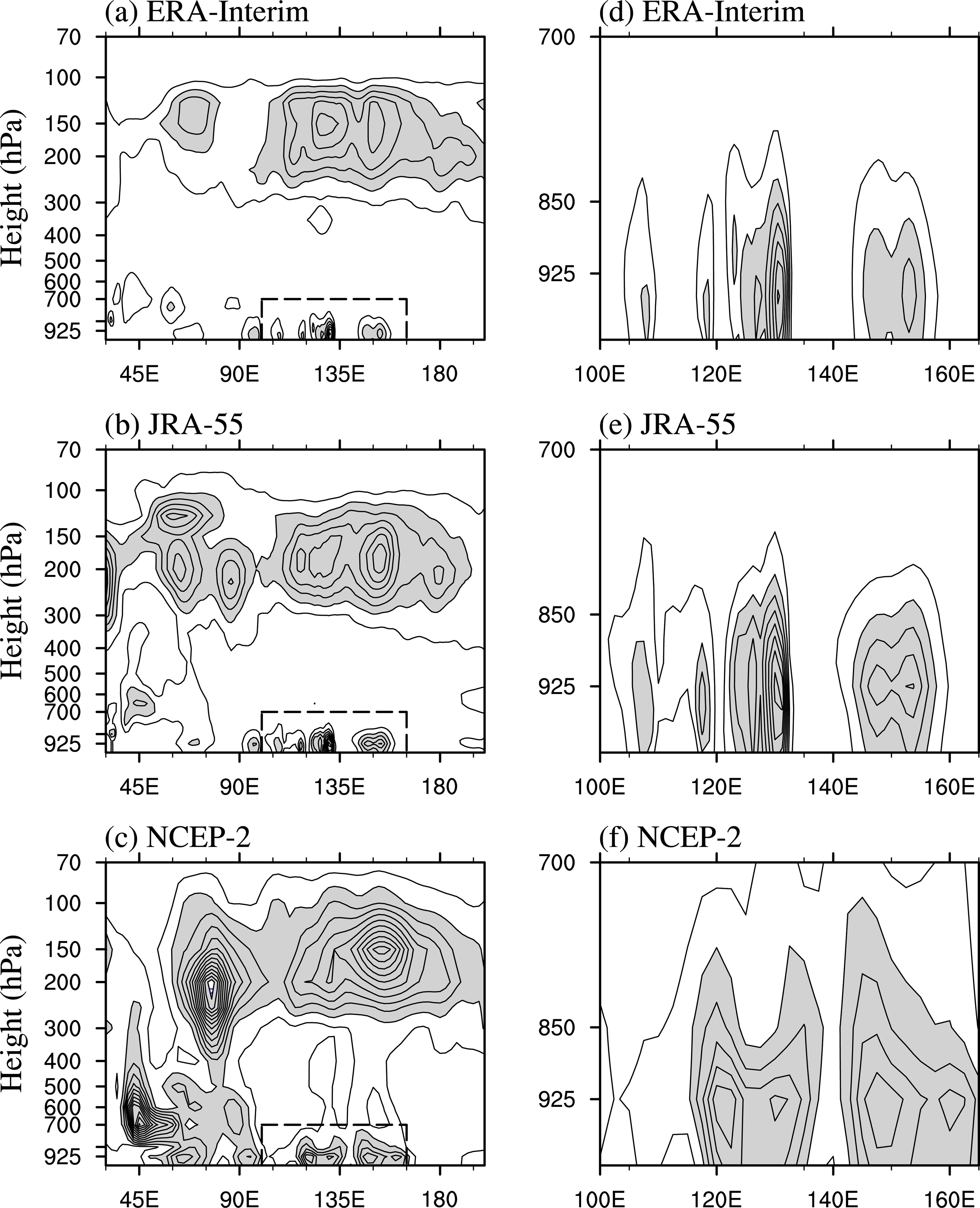 Figure2. Variance of meridional winds along the equator based on (a) ERA-Interim, (b) JRA-55, and (c) NCEP-2. The contour interval is 0.4 m2 s?2, and the zero contours are omitted. The regions framed by the rectangle in (a?c) are magnified to (d?f), respectively. The shaded regions represent values greater than 0.8 m2 s?2.
However, there are large differences in variance between the datasets. First, variances show strong differences to the west of 90°E. They are much greater in JRA-55 and NCEP-2 at the upper levels in comparison with ERA-Interim. In addition, the large values shown at the western edge of Fig. 2b extend to 10°E, with the maximum locating around 30°E (not completely shown in Fig. 2b), and these strong variances are related to the decadal time scale (Fig. 3b). Furthermore, there are two cores of strong variance in the upper troposphere and mid?lower troposphere for NCEP-2 (Fig. 2c), which are absent for ERA-Interim (Fig. 2a). Second, in the upper troposphere over the Maritime Continent, variances are characterized by one core at 150°E for NCEP-2 but by several cores for ERA-Interim and JRA-55. Third, in the lower troposphere over the Maritime Continent, which is highlighted in Figs. 2d-f, variances measured by JRA-55 are stronger than in ERA-Interim, and strong variances tend to appear over larger scopes in NCEP-2 than in the other two datasets.
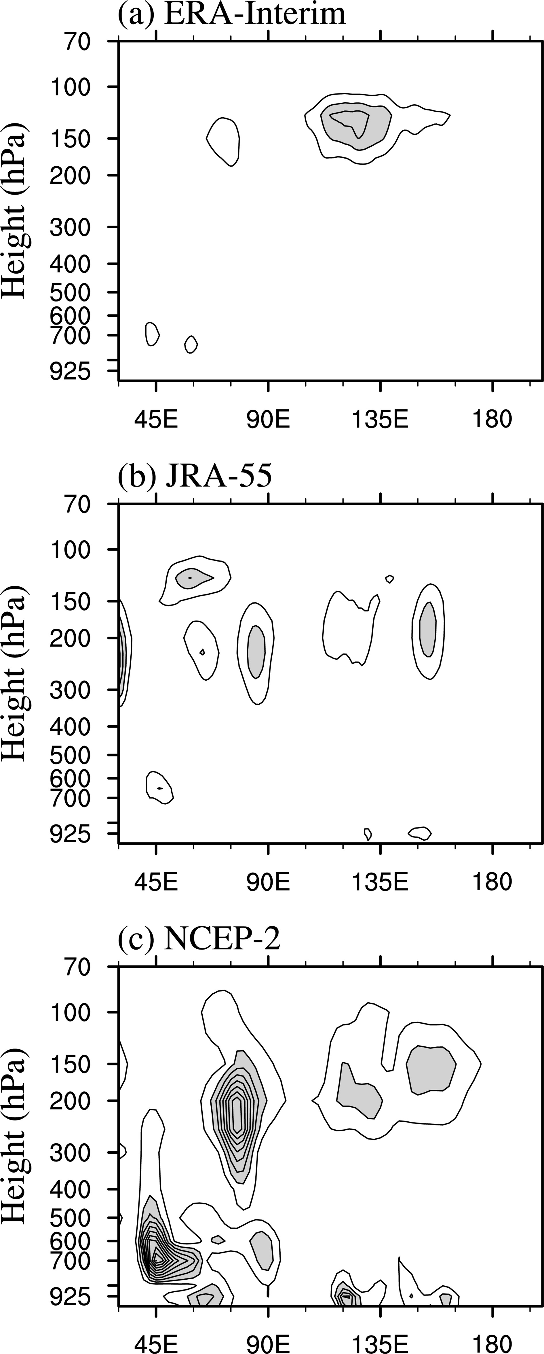 Figure3. Variance of the interdecadal component of meridional winds along the equator based on (a) ERA-Interim, (b) JRA-55, and (c) NCEP-2. The contour interval is 0.4 m2 s?2, and the zero contours are omitted. The shaded regions represent values greater than 0.8 m2 s?2.
Figure 3 shows the variance of meridional winds along the equator on the decadal time scale. Large differences can be found between the datasets. Variances are greater in JRA-55 and NCEP-2 at the upper levels to the west of 90°E than in ERA-Interim. In addition, there are two cores of strong variance in the upper troposphere and mid?lower troposphere for NCEP-2 (Fig. 3c). Furthermore, NCEP-2 shows larger variances at both the upper and lower levels over the Maritime Continent. These differences in variance between the datasets are roughly consistent with those for total variance shown in Fig. 2, implying that decadal variance contributes significantly to the differences in total variance between the datasets.
The interannual variance (Fig. 4) is much more consistent between the datasets. To the west of 90°E, variances are strong in the upper troposphere and weak in the lower troposphere, although the strong variances in the upper troposphere appear further eastward in NCEP-2 in comparison with the two other datasets. Over the Maritime Continent, strong variances appear both in the upper troposphere and at lower levels for all the datasets. In the upper troposphere, the interannual variation is consistently large from 110°E to 170°E, although for NCEP-2 strong variances tend to be concentrated around 150°E. In the lower troposphere over the Maritime Continent (Figs. 4d-f), large variances are also very similar in both intensity and distribution, though JRA-55 shows slightly larger values and NCEP-2 shows weaker values and a smoother distribution. These strong variances are roughly consistent with the strong prevailing southerlies shown in Fig. 1, but with appreciable differences. For instance, at around 150°E the climatological southerlies are weak, while the variances are strong. All the datasets show very weak variances in the domain of the Somali jet. These consistent features of interannual variance and large differences in decadal variance suggest that the distinctions in total variance mainly result from the decadal variability.
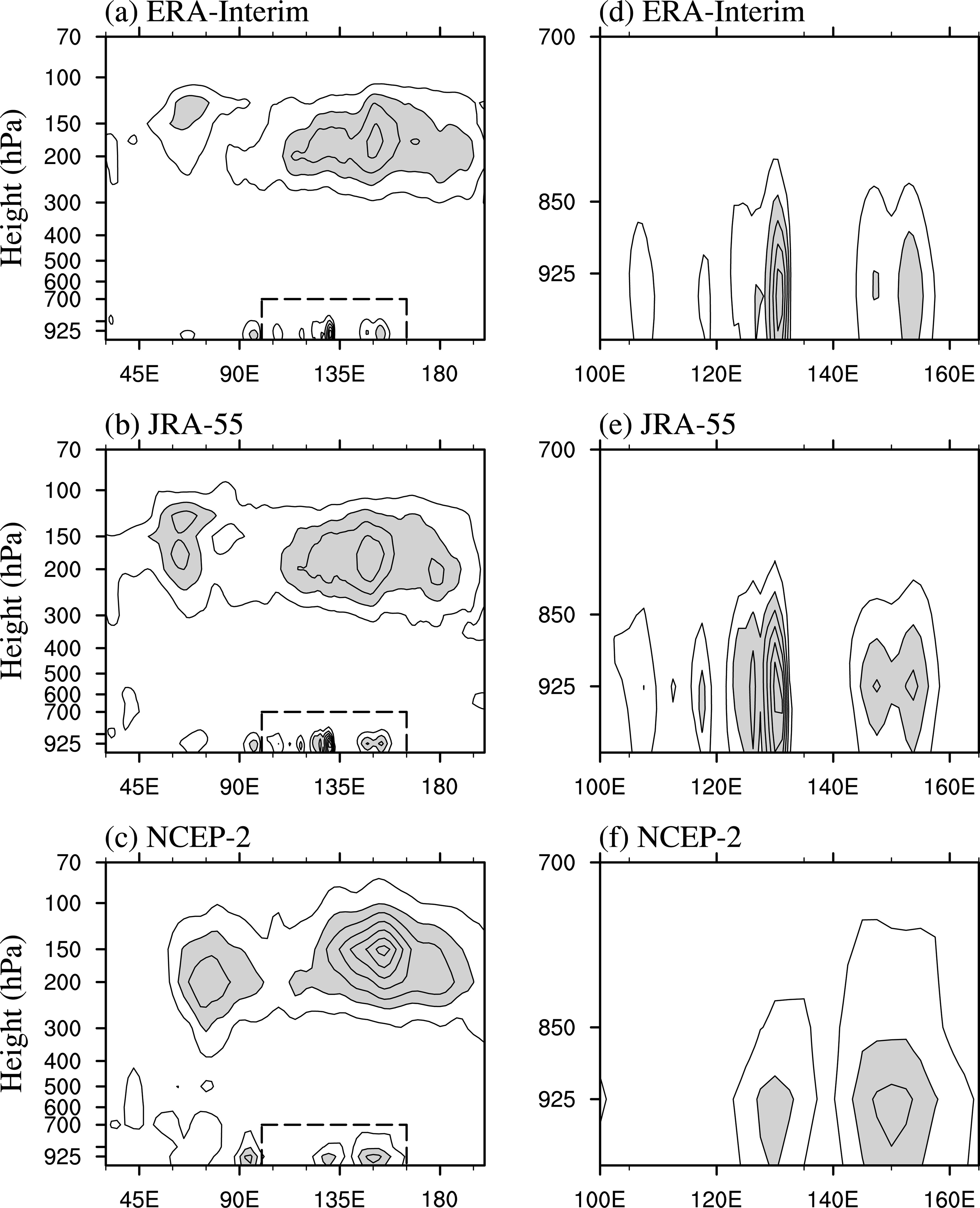 Figure4. As in Fig. 2 but for the interannual component.
To more clearly illustrate the consistency among the three datasets in depicting the interannual variability, we show in Fig. 5 the ratios of the interannual standard deviation of the equatorial meridional winds between the datasets. The domains where the ratios are greater than 1.25 or lower than 0.8 are dotted and checked, respectively, and the consistency of the interannual variability between the datasets is highlighted by the blank areas. The strongest consistency appears between ERA-Interim and JRA-55, indicated by the largest blank area in Fig. 5a, which extends from the upper troposphere downward to the lowest level from 90°E to 165°E. Consistency also appears in the upper troposphere over the Maritime Continent, particularly around 200 hPa, between NCEP-2 and the other two datasets (Figs. 5b and c). Consistency tends to exist at 925 hPa around 130°E and 150°E, where the interannual variance is relatively larger (Fig. 4).
 Figure5. Ratio of the interannual standard deviation of meridional winds between (a) ERA-Interim and JRA-55, (b) ERA-Interim and NCEP-2, and (c) JRA-55 and NCEP-2. The isolines represent the values of 1.25 and 0.8. Values less than 0.8 are marked by checks, and those larger than 1.25 are marked by dots.
Figure 6 shows the vertical?longitude section of the correlation coefficient of the interannual variations in equatorial meridional winds between the datasets. Only two contours, i.e., 0.85 and 0.95, are shown in this figure to highlight the domains of high correlation. The strongest consistency appears between ERA-Interim and JRA-55, both in the upper troposphere and in the lower levels over the Maritime Continent, in agreement with the high consistency in interannual standard deviation (Fig. 5a). High correlation coefficients appear from 90°E to 170°W in the upper troposphere, centered at about 200 hPa (Fig. 6a). In the lower levels, on the other hand, high correlations are centered around 105°E, 130°E and 150°E, respectively (Fig. 6d), which is closely consistent with the three branches of relatively larger interannual variance (Figs. 4d and e). Furthermore, high correlations also appear in the upper troposphere and over the three branches in the lower levels over the Maritime Continent between NCEP-2 and the other two datasets (Figs. 6b, c, e and f). These high correlations exhibit a very similar distribution in comparison with those between ERA-Interim and JRA-55 (Figs. 6a and d), although showing a weak intensity.
 Figure6. Correlation coefficients of the equatorial meridional winds on the interannual time scale between (a) ERA-Interim and JRA-55, (b) ERA-Interim and NCEP-2, and (c) JRA-55 and NCEP-2. The isolines represent the values of 0.85 and 0.95. Regions shaded gray denote values greater than 0.95. The regions framed by the rectangle in (a?c) are magnified to (d?f), respectively.
So far, we have illustrated the vertical structure of the climatology and variability of CEFs and validated that the three datasets have higher consistency on the interannual time scale, especially between ERA-Interim and JRA-55, while the interdecadal component varies widely. Thus, further investigation in this study will mainly focus on the interannual variability.
The meridional wind anomalies regressed onto the MC-LCEFI are shown in Fig. 7. There are significant northerly anomalies in the upper troposphere and southerly anomalies in the lower levels of the troposphere over the Maritime Continent in all datasets. This indicates a strengthening of both the upper and lower branches of CEFs over the Maritime Continent. The northerly anomalies consistently appear between 90°E and 170°E around 200 hPa, with the strongest one at about 150°E. Although we define the MC-LCEFI using the three branches to the east of 100°E, there are also significant southerly anomalies between 90°E and 100°E in the lower troposphere. Weak but significant southerly anomalies appear in the mid troposphere over the Maritime Continent in both ERA-Interim and JRA-55, but these are absent in NCEP-2. In addition, to the west of 90°E, there are southerly anomalies in the upper troposphere and northerly anomalies in the lower levels. The upper-tropospheric southerly anomalies are very similar between ERA-Interim and JRA-55, but shift eastward in NCEP-2. The low-level northerly anomalies are significant, and this out-of-phase relationship between the Somali jet and the MC-LCEFs has been well documented by Li and Li (2014), Li et al. (2017a), and Li et al. (2017b). However, the anomalies associated with the Somali jet are much weaker, consistent with the weak interannual variance (Fig. 4), and they appear relatively eastward in NCEP-2.
 Figure7. Regression of the interannual component of the meridional winds along the equator onto the lower-level MC-CEF index based on (a) ERA-Interim, (b) JRA-55, and (c) NCEP-2. The contour interval is 0.2 m s?1, and the zero contours are omitted. The red (blue) shading denotes positive (negative) values, and dots represent regions significant at the 95% confidence level based on the Student’s t-test.
This negative relationship between the upper and lower troposphere over the Maritime Continent can also be confirmed from the viewpoint of upper-tropospheric CEFs. Figures 8a-c show the correlation coefficients of equatorial meridional winds between the reference point (200 hPa, 150°E) and all the grids. This reference point shows the strongest meridional wind anomaly associated with the low-level CEFs (Figs. 7a and b) and the greatest interannual variance (Figs. 4a and b) in ERA-Interim and JRA-55. The correlation coefficients over the Maritime Continent are characterized by positive values in the upper troposphere and negative ones in the lower levels in all the datasets. Strong negative correlations in the lower levels are centered in several branches, consistent with the large interannual variance (Figs. 4d-f). Besides, there are negative and positive correlations to the west of 90°E in the upper and lower troposphere, centered around 150 hPa and 850 hPa, respectively. This distribution is very similar to that shown in Fig. 7, including the negative correlations (Fig. 8) and southerly anomalies (Fig. 7) in the mid troposphere over the Maritime Continent, in ERA-Interim and JRA-55 but not in NCEP-2.
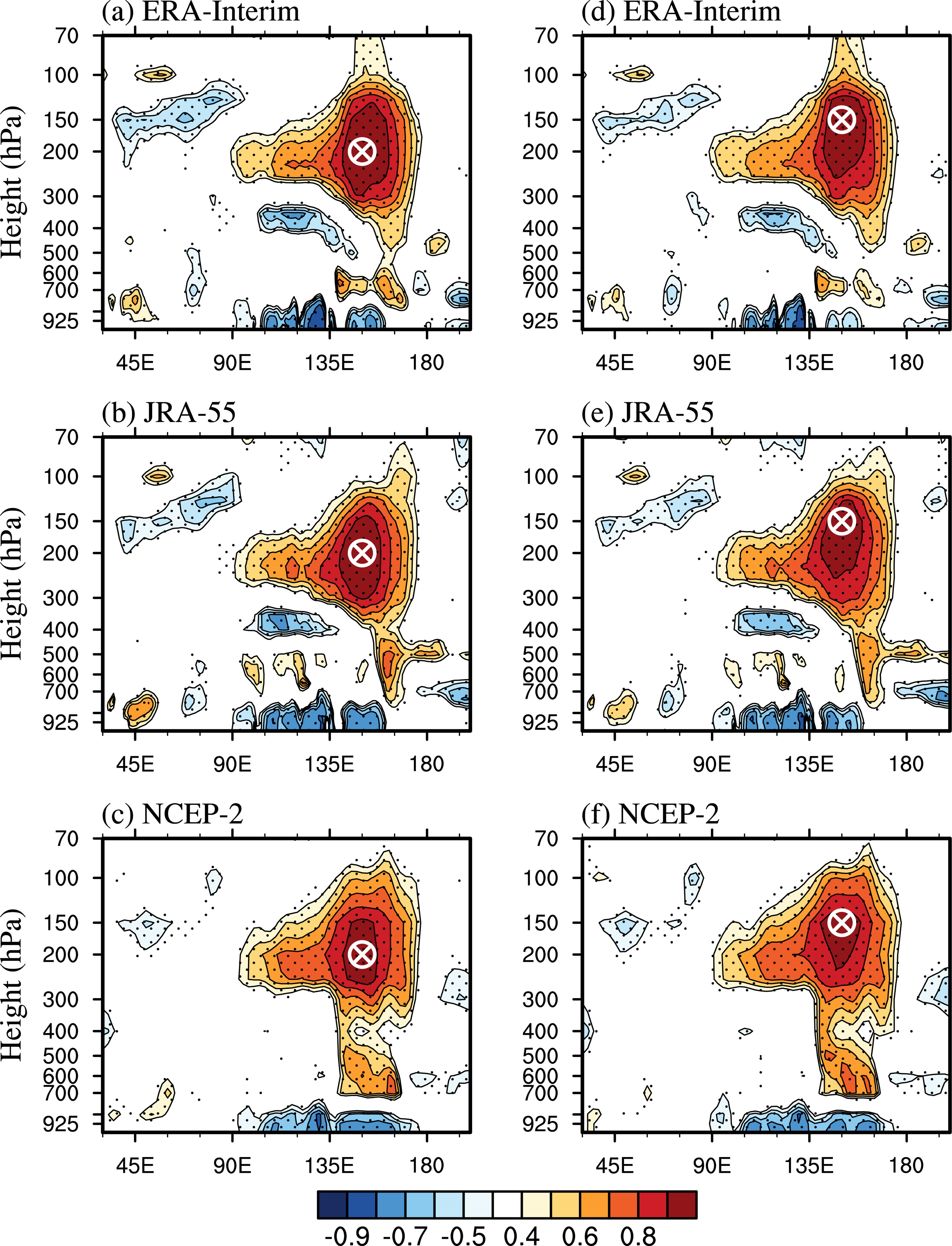 Figure8. One-point correlation coefficient for the interannual component of the meridional winds along the equator based on (a) ERA-Interim, (b) JRA-55, and (c) NCEP-2. The reference point (200 hPa, 150°E) is marked by the white cross. The contour interval is 0.1, and values between ?0.4 and 0.4 are omitted. The red (blue) shading denotes positive (negative) values, and dots represent regions significant at the 95% confidence level based on the Student’s t-test. As in (a?c) (d?f) are for the reference point (150 hPa, 150°E).
Considering that the strongest interannual variance and northerly anomaly in NCEP-2 appear at 150 hPa (Figs. 4c and 7c), we use (150 hPa, 150°E) as the reference point and repeat the analysis. The results (Figs. 8d-f) are similar, and the largest positive values appear at 200 hPa to the west of 135°E, even though the reference point is shifted to 150 hPa.
The above results demonstrate the significant negative relationship in the equatorial meridional winds between the upper and lowest level of the troposphere, over the Maritime Continent and Indian Ocean. The domains of significant correlation are closely consistent with those of large interannual variance. All these results imply that the negative relationship may play an important role in the interannual variability of the equatorial meridional winds over the Maritime Continent and Indian Ocean. To verify this, we perform an EOF analysis on the equatorial meridional winds in the domain of (30°E?160°W, 1000?70 hPa), which is the same as those for Figs. 4, 7 and 8. The first mode (EOF1) is separable from the other modes according to North et al. (1982), and accounts for 34.3%, 32.5% and 29.2% of the total interannual variance in ERA-Interim, JRA-55 and NCEP-2, respectively. Figure 9 shows the equatorial meridional wind anomalies regressed onto the standardized principal component of the first mode (PC1). EOF1 is characterized by northerly (southerly) anomalies in the upper (lower) troposphere over the Maritime Continent and southerly anomalies in the upper troposphere over the Indian Ocean in all the datasets. There are also significant, albeit weak, anomalies of the Somali jet. This distribution resembles very well the distributions shown in Figs. 7 and 8.
 Figure9. Regression of the interannual component of the meridional winds along the equator onto the normalized PC1, with the EOF analysis performed for the domain identical to that shown in the figure, based on (a) ERA-Interim, (b) JRA-55, and (c) NCEP-2. The contour interval is 0.2 m s?1, and the zero contours are omitted. The red (blue) shading denotes positive (negative) values, and dots represent regions significant at the 95% confidence level based on the Student’s t-test.
To compare the first mode and these significant meridional wind anomalies over the Maritime Continent and Indian Ocean, we define several indexes to depict the meridional wind anomalies. First, considering the distribution of the anomalies over the Maritime Continent shown in Figs. 7 and 8 and the large variances shown in Fig. 4, we define MC-HCEFI as the standardized JJA-mean equatorial meridional winds at 200 hPa averaged over 110°?170°E. Second, we define IO-HCEFI at 150 hPa over 45°?75°E along the equator based on a similar consideration. Third, as mentioned before, we define MC-LCEFI, following Li and Li (2014), but only the equatorial winds are used here. We also follow Li and Li (2014) and define the Somali jet index (Somali-I) by averaging the equatorial meridional winds at 850 hPa over 37.5°?62.5°E.
Figure 10 shows the interannual and decadal variations of these indexes. High consistency exists among the three datasets in depicting the interannual variability in the upper troposphere and low-level branches over the Maritime Continent (Figs. 10a and b), consistent with the results shown in the preceding section. For instance, the correlation coefficient between ERA-Interim and JRA-55 is 0.98 for MC-HCEFI and 0.99 for MC-LCEFI. The similarity among different datasets over the Indian Ocean on the interannual time scale, albeit weaker than that over the Maritime Continent, can also be found from the series of IO-HCEFI and Somali-I (Figs. 10c and d), with the correlation coefficient being 0.88 for IO-HCEFI and 0.92 for Somali-I. In contrast, the decadal indexes show large differences (Figs. 10e-h). ERA-Interim and JRA-55 tend to show consistent decadal variations of the low-level CEFs over the Maritime Continent (Fig. 10f), but they show quite different variations of the high-level MC-CEF and the CEFs over the Indian Ocean (Figs. 10e, g and h). The large differences shown by the decadal indexes indicate that there is great uncertainty in the decadal variations of CEFs over the Maritime Continent and Indian Ocean in the current reanalysis data.
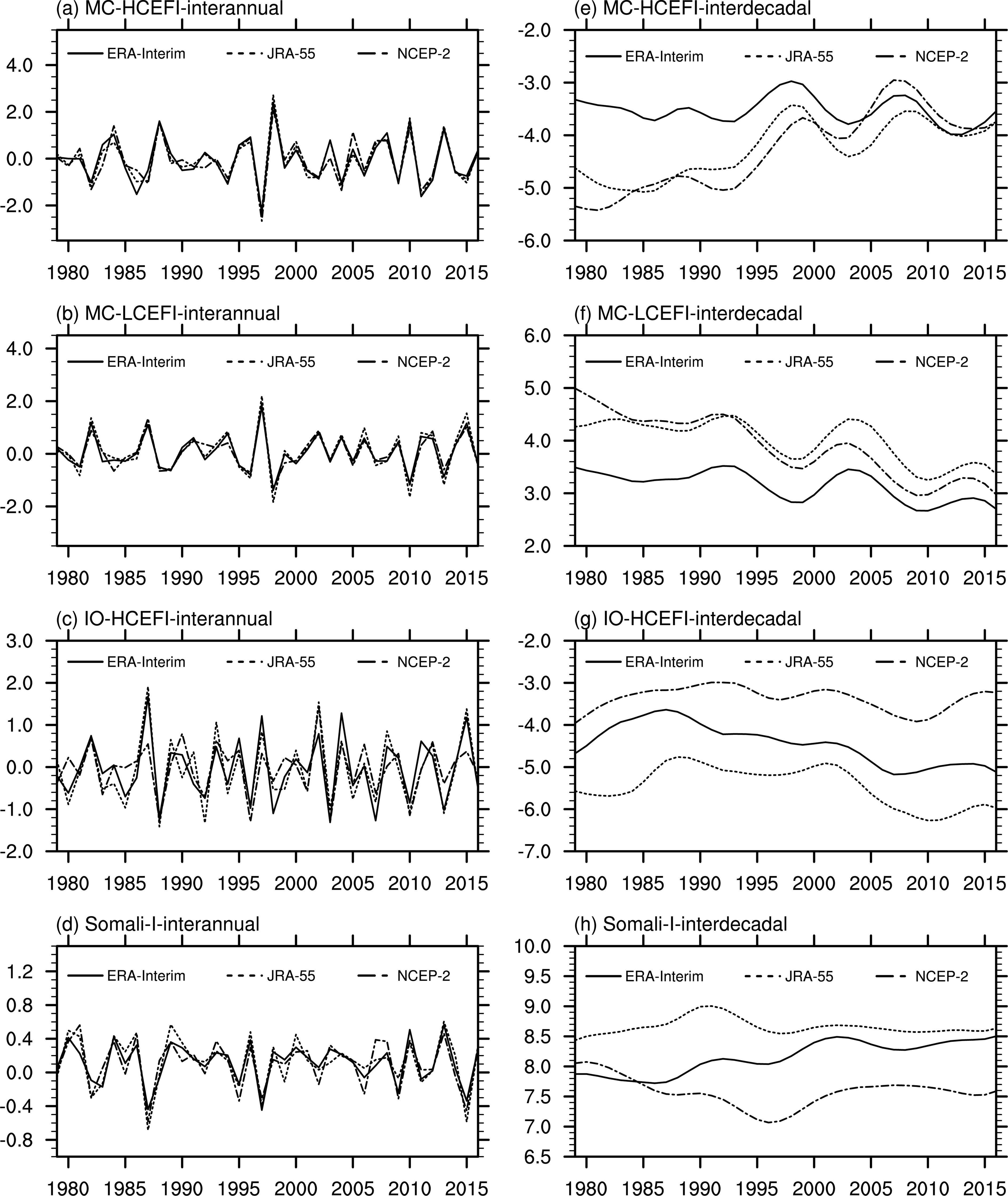 Figure10. Time series of (a) MC-HCEFI, (b) MC-LCEFI, (c) IO-HCEFI, and (d) Somali-I calculated by the interannual component based on ERA-Interim, JRA-55 and NCEP-2. As in (a?d) (e?h) are for the interdecadal component.
We calculate the correlation coefficients between PC1 and these indexes and show them in Table 1. PC1 is highly correlated with MC-HCEFI and MC-LCEFI, suggesting that the first mode can explain the majority of the interannual variance of CEFs in both the upper and lowest level of the troposphere over the Maritime Continent. In addition, PC1 is also significantly correlated with IO-HCEFI and Somali-I. These correlation coefficients confirm the close relationship between the first mode and CEFs over the Maritime Continent and Indian Ocean. Or, in other words, the relationship between the CEFs over the Maritime Continent and Indian Ocean, particularly the seesaw pattern between the upper and lower troposphere over the Maritime Continent, contributes significantly to the first mode.
| Index | MC-HCEFI | MC-LCEFI | IO-HCEFI | Somali-I | PC1 |
| MC-LCEFI | ?0.86 | ? | ? | ? | ? |
| IO-HCEFI | ?0.61 | 0.72 | ? | ? | ? |
| Somali-I | 0.48 | ?0.68 | ?0.55 | ? | ? |
| PC1 | ?0.98 | 0.93 | 0.68 | ?0.59 | ? |
| Ni?o3.4 | ?0.67 | 0.83 | 0.68 | ?0.62 | 0.75 |
Table1. Correlation coefficients between the indexes used in this study based on ERA-Interim. Results based on JRA-55 and NCEP-2 are very similar with ERA-Interim and are therefore not shown here.
In addition, a strong relationship between CEFs and ENSO, especially for MC-CEF, can be found in Fig. 10. For example, MC-HCEFI reaches a minimum (maximum) in 1997 (1998), which was a developing summer for a strong El Ni?o (La Ni?a). This relationship can be verified by the correlation coefficients with the Ni?o3.4 index (Table 1), which is defined as the standardized JJA-mean SST anomalies averaged over (5°S?5°N, 120°?170°W), using the monthly mean SST data provided by ERSST.v5. Actually, the Ni?o3.4 index is also highly correlated with PC1 (0.75; Table 1). All these strong correlation coefficients suggest that ENSO may contribute much to the leading mode. To confirm this, we regress the equatorial meridional wind anomalies onto the JJA-mean Ni?o3.4 index, and show the results in Fig. 11. Over the Maritime Continent there are northerly anomalies in the upper troposphere and southerly anomalies in the low-level branches. There are also southerly anomalies in the upper troposphere over the Indian Ocean and weak northerly anomalies in the lower troposphere around 50°E. This distribution is closely consistent with the leading mode shown in Fig. 9. All these results indicate that ENSO contributes much to the leading mode of equatorial meridional winds and the linkage between CEFs in the upper and lower troposphere over the Maritime Continent and Indian Ocean. The ENSO-related meridional wind anomalies tend to appear over a relatively narrow scope around 200 hPa in the vertical direction over the Maritime Continent, in comparison with those associated with PC1 (Fig. 9), indicating that ENSO is most strongly correlated with CEFs at 200 hPa and thus providing an extra advantage of defining CEFs by using 200-hPa meridional winds.
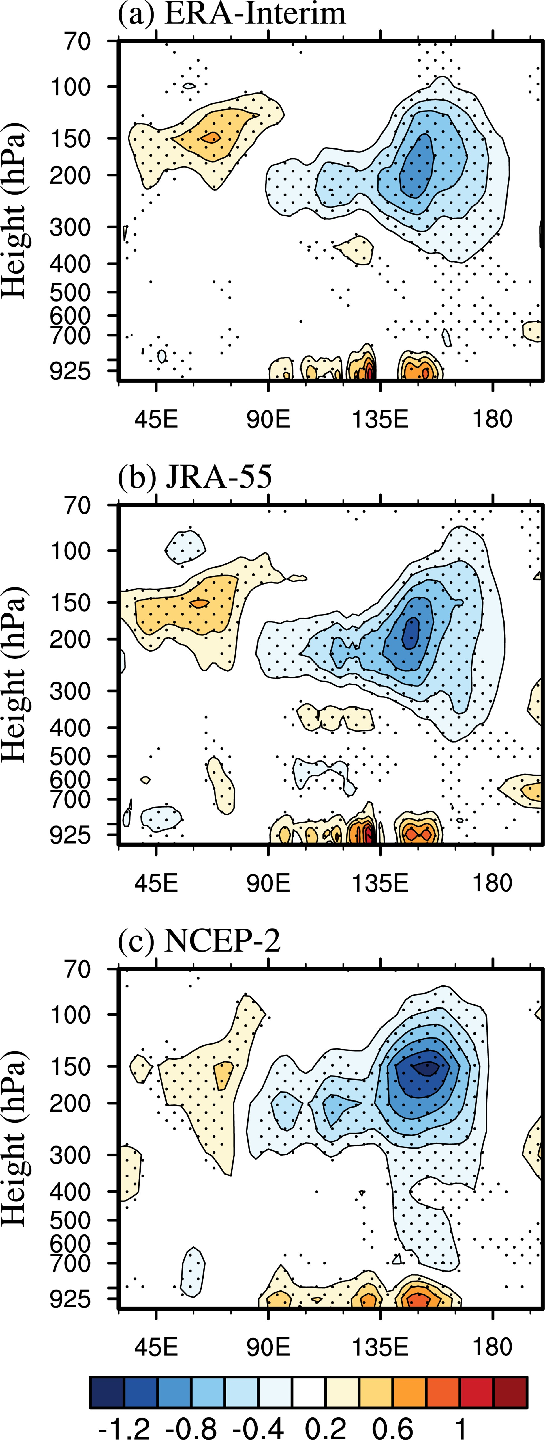 Figure11. Regression of the interannual component of the meridional winds along the equator onto the Ni?o3.4 index in JJA based on (a) ERA-Interim, (b) JRA-55, and (c) NCEP-2. The contour interval is 0.2 m s?1, and the zero contours are omitted. The red (blue) shading denotes positive (negative) values, and dots represent regions significant at the 95% confidence level based on the Student’s t-test.
Further analysis is performed to illustrate the vertical structure of the interannual variability in CEFs over the Maritime Continent and Indian Ocean. The results show that there is a significant negative relationship between the upper and lowest-tropospheric CEFs over the Maritime Continent, i.e., enhanced cross-equatorial southerly flows in the low levels correspond to intensified northerly flows in the upper levels. In other words, CEFs are enhanced simultaneously in both the lower and upper branches over the Maritime Continent. This seesaw pattern over the Maritime Continent is also significantly related to CEFs over the Indian Ocean: enhanced CEFs over the Maritime Continent correspond to weakened CEFs over the Indian Ocean—that is, both the Somali jet in the lower levels and returning northerly flows in the upper levels are weakened. This correspondence in CEFs, both zonally and vertically, is manifested as the leading mode of equatorial meridional winds over the Maritime Continent and Indian Ocean. Finally, it is found that ENSO is closely related to the vertical structure of the interannual variability in CEFs over the Maritime Continent and Indian Ocean. The summer Ni?o3.4 index is significantly correlated to the leading mode and lower- and upper-level CEFs over the Maritime Continent and Indian Ocean. This suggests that ENSO may contribute remarkably to the vertical structure of the interannual variability in CEFs over the Maritime Continent and Indian Ocean.
This study reveals the vertical structure of CEFs over the Maritime Continent and Indian Ocean on the interannual time scale and the effect of ENSO on the vertical structure. Associated with the vertical structure, CEFs shows close relationships between the lower and upper branches, and between the Maritime Continent and Somali jet. This is partially consistent with previous studies, which have demonstrated the relationship between lower-level CEFs over the Maritime Continent and the Somali jet (Li and Li, 2014). This study, however, does not examine the horizontal distribution of circulation anomalies associated with the vertical structure of CEFs. The horizontal distribution of circulation anomalies can help us better understand the climate anomalies associated with the variability of CEFs and the physical mechanisms underlying their variability. Therefore, further analyses on this issue are required in the future.
Based on the present results, we suggest that using 200-hPa meridional winds is a good choice to define the upper-level CEFs over the Maritime Continent in consideration of the following facts. First, at this pressure level, CEFs are roughly strongest in climatological terms and show the greatest interannual variability over the Maritime Continent. Therefore, the definition can appropriately depict the variability of CEFs. Second, the meridional winds at this level are most strongly related to both the leading mode and ENSO, and the significant meridional wind anomalies occupy the largest zonal scope over the Maritime Continent. Finally, around 200 hPa, the three reanalysis datasets show their highest consistency in depicting the interannual variability of meridional winds along the equator. On the other hand, 150 hPa is suggested for the definition of upper-level CEFs over the Indian Ocean, for similar reasons.
Acknowledgements. This research was supported by the National Natural Science Foundation of China (Grant No. 41721004).
