HTML
--> --> -->CH4 is one of the most important carbon-containing compounds in the atmosphere. The global warming potential (GWP) of CH4 is 28 times greater than that of CO2 (IPCC, 2014). In addition, it is a chemically active gas, which can be oxidized in the atmosphere to form hydroxides and carbon oxyhydroxides. Stratospheric CH4 can also react with chlorine atoms generated by photolysis of chlorofluorocarbons, inhibiting the destruction of stratospheric ozone by chlorine atoms (Duncanand Truong, 1955). The lifetime of CH4 in the atmosphere is approximately nine years (Kirschke et al., 2013). Considering the GWP and lifetime of CH4, it is important to study the sources and sinks of CH4 to learn how to control it.
Generally, sources of CH4 can be divided into two types: natural and anthropogenic. Natural sources include wetlands, vegetation, and oceans (Fung et al., 1991). Anthropogenic sources include energy activities (involving coal mining and oil and gas systems), agricultural activities (involving ruminants, rice field discharge, and open burning of straw), waste treatment (of solid waste, industrial waste, and domestic sewage) and constructed wetlands (Janssens-Maenhout et al., 2019). The destructive reaction with the hydroxyl radical (OH) is the biggest sink of CH4 in the atmosphere, especially in the troposphere (Heilig, 1994).
Systematic observation of CH4 began in the 1880s via the Global Atmospheric Watch (GAW) of the World Meteorological Organization (WMO). Currently, the ground-based high-resolution Fourier transform infrared (FTIR) solar absorption spectrometer plays an important role in remote sensing of trace gases. There are two CH4 observation networks in the world: one is the Total Carbon Column Observing Network (TCCON) (Wunch et al., 2011), and the other is the Network for the Detection of Atmospheric Composition Change-Infrared Working Group(NDACC-IRWG) (De Mazière et al., 2018). Both networks exist in Europe, North America, and Japan, and there is currently only one potential additional TCCON site (in Hefei), and no NDACC site in China. In this study, the temporal and vertical distributions of CH4were measured by both the FTIR in-situ techniques at a new site in Xianghe, China.
 Figure1. (a) EDGAR v4.3.2 CH4 anthropogenic emissions in 2012 in China. (b) Annual total Chinese CH4 emissions contributed by eightsectors in 1970–2012.
We began measuring CH4 in June 2018. The sources of CH4 are relatively variable and location-dependent. In most parts of the world, natural emissions are the main sources, such as wetlands, termites, oceans, and hydrates (Kaplan et al., 2006; IPCC, 2014; Zhang and Liao, 2015). However, more recently, anthropogenic emissions have come to play an important role (Kirschke et al., 2013). Fugitive emissions from solid fuels, rice cultivation and enteric fermentation are very important in China (Fig. 1b).
3.1. Picarro G2301
The Picarro G2301 gas mole fraction analyzer provides simultaneous and precise measurements of CO2, CH4, and H2O, with a sensitivity of 1 ppb and negligible drift. This instrument is widely used in atmospheric science and air quality applications for quantification of emissions. The G2301 uses WS-CRDS (wavelength-scanning cavity ring-down spectroscopy) to measure the laser ring-down time difference over a path length of up to 20 km with high accuracy (Fang et al., 2012). It meets the WMO and ICOS (Integrated Carbon Observation System) performance requirements for CO2 and CH4 atmospheric monitoring (Laurent, 2015). The G2301 was fully operational, almost without interruption, during the study period. We use 5-min-averaged CH4 data at the surface (90 mMSL) to ensure high accuracy (< 0.7 ppb).2
3.2. FTIR spectrometer
We used the Bruker IFS 125HR FTIR to observe CH4 in Xianghe, which is the highest-precision instrument among ground-based remote sensing instruments (± 0.9 ppb; Esler et al., 2000). The maximum optical path difference of the FTIR in Xianghe was 180 cm, with a spectral resolution of 0.0035 cm?1. To obtain more observations of trace gases, we used two observation modes: TCCON and NDACC-IRWG. NDACC-IRWG adopts a CaF2 beam splitter and an InSb detector with a spectral range of 1800–5400 cm?1, while TCCON uses CaF2 and InGaAs with a spectral range of 3900–12000 cm?1. The FTIR works during the day [between 0900 and 1600 local time (LT)]. For each day, there are approximately 40 spectra measured in TCCON observation mode and 5 measured in NDACC observation mode, and these are used to retrieve CH4. Figure 2 shows the typical spectra measured by the two modes. The TCCON and NDACC retrieval strategies, i.e., retrieval windows and interfering species, are shown in Table 1. A specific filter is applied for the InSb spectrato increase the signal-to-noise ratio.| Observation modes | TCCON | NDACC |
| Algorithm | GGG2014 | SFIT4 |
| Retrieval windows (cm?1) | 5872.0–5988.0 5996.45–6007.55 6007.0–6145.0 | 2611.6–2613.35 2613.7–2615.4 2835.55–2835.8 2903.82–2903.925 2941.51–2942.22 |
| Interfering species | CO2, H2O, N2O | H2O, HDO,CO2, NO2 |
| A priori profile | TCCON tool (daily) | WACCM v4 |
| Products | Total column | Profile |
Table1. TCCON and NDACC CH4 retrieval strategies in Xianghe.
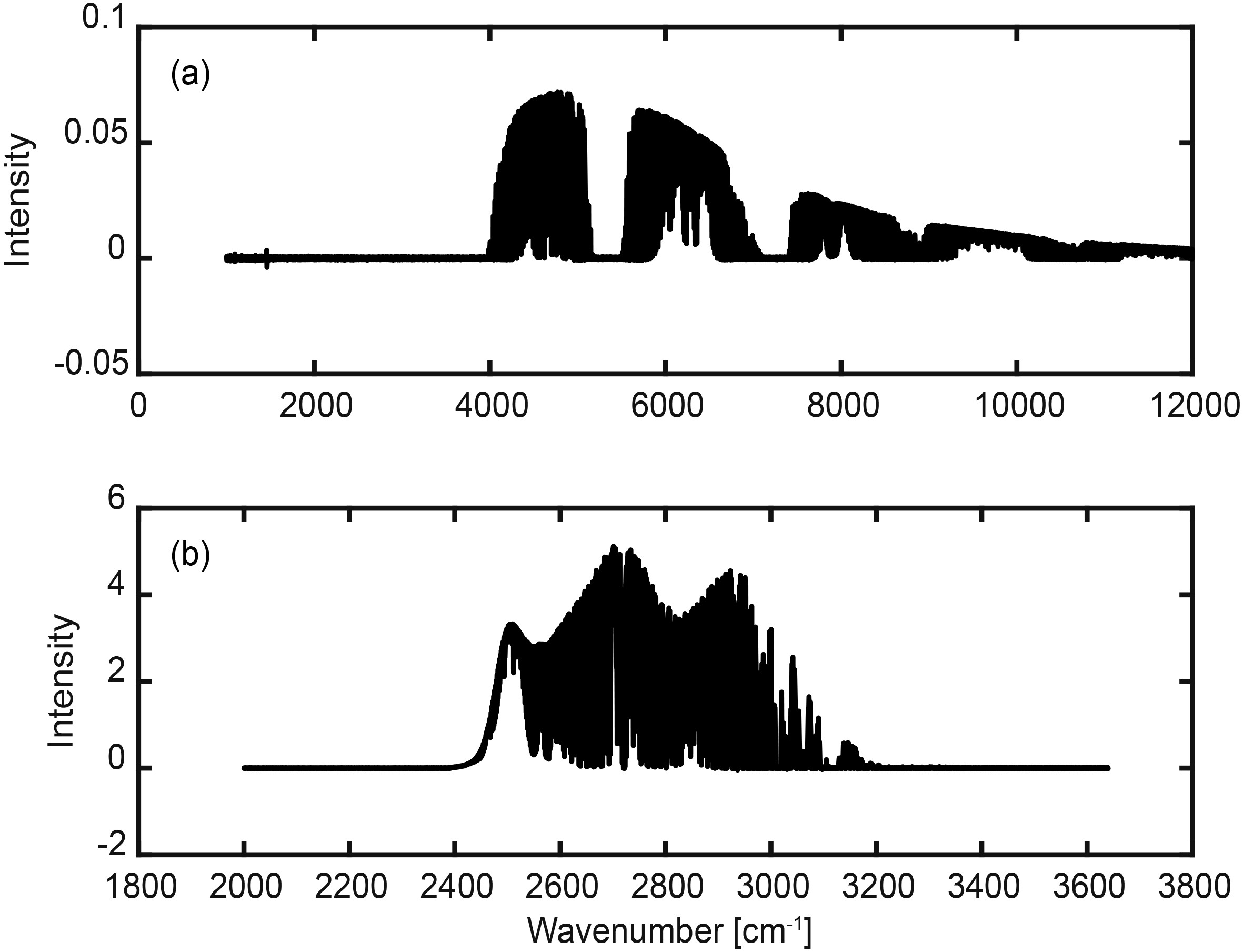 Figure2. Spectrum observed by FTIR with (a) InGaAs detector and (b) InSb detector.
3
3.2.1. Retrieval method
The optimal estimation method (Rodgers, 2000) was applied to retrieve gas mole fractions from the FTIR solar spectra. Several software retrieval algorithms are applied for different purposes, such as GGG2014, SFIT, and PROFFIT (Toon et al., 1992; Notholt et al., 1993; Hase et al., 2004).According to the optimal estimation method, atmospheric radiation transfer can be described by a simple mathematical model, as follows:
where Y is the radiation spectrum, X is the set of unknown atmospheric and surface state quantities, as well as the solar and instrumental parameters that affect the radiation spectrum, b is the set of known atmospheric and surface state parameters, F is the forward-transfer radiation model function, and ε is the error of observation. The inversion process involves taking the observed spectrum (Y) and finding the unknown atmospheric and surface state parameters (X).
To carry out the inversion process, a cost function is defined as:
where the first term on the right-hand side represents the difference between the measured and simulated spectra for a given atmospheric state of X and b,


where


In Eq. (4), G is called the contribution function matrix, which indicates the contribution of observed values to inversion values, K is a weight function matrix that expresses the sensitivity of simulated values to input parameters, such as the instrument line functions, and

3
3.2.2. GGG2014 and SFIT4 retrievals
The GGG2014 algorithm was applied to retrieve the column-averaged dry-air mole fraction of CH4 (


where 0.2095 is the volume mixing ratio of O2 in dry air (Wunch et al., 2011).
Since there is no O2 signal available in the mid-infrared spectrum, and the N2 signal is very weak (Zhou et al., 2018), the SFIT4 algorithm calculates the

where


Note that the a priori information is different between GGG2014 and SFIT4. For the meteorological variables of temperature, pressure, and water vapor, both algorithms use NCEP six-hourly reanalysis data. However, the a priori profiles of CH4 are obtained by different methods. For GGG2014, the daily profiles are generated by a stand-alone tool based on in-situ and aircraft measurements (Toon and Wunch, 2015). For SFIT4, the profiles are derived from the Whole Atmosphere Community Climate Model (WACCM), version 4 (Zhou et al., 2019).
Figure 3 shows information about the AVK in GGG2014 and SFIT4 for different solar zenith angles (SZAs). The AVK represents the sensitivity of the inversion to the true state of the atmosphere (see section 3.2.1). Ideally, the AVK is an identity matrix, indicating that the inversion is sensitive to the whole atmosphere. However, in reality, the sensitivity to the atmospheric state of the AVK varies by height. For example, for TCCON, the total amount of CH4 is always sensitive to the troposphere (> 0.8), regardless of SZA. However, in the stratosphere, the total amount of CH4 varies from 1.2 to 0.6 as the SZA varies from 10° to 85°.
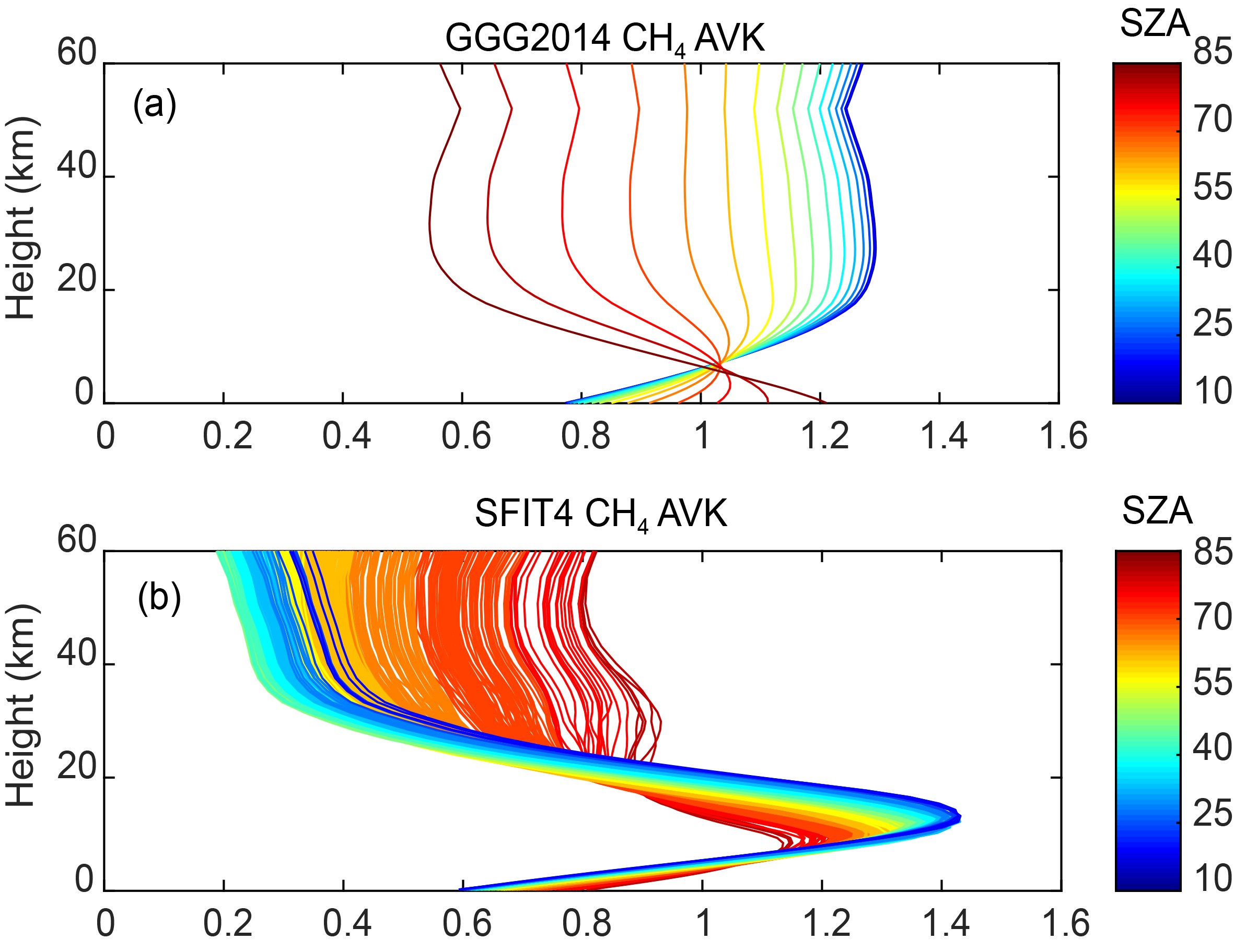 Figure3. Column averaging kernel (AVK) of the CH4 retrieval in the (a) GGG2014 and (b) SFIT4 codes, colored with different solar zenith angels (SZAs).
This is mainly because, as the Sun obliquely enters the atmosphere (as SZA increases), pressure broadening in the stratosphere contributes to a narrower linewidth than the saturated central region for gases with saturated absorption lines. Therefore, as the mass of air increases, the line becomes more saturated, so the AVK of the stratosphere is partially reduced, resulting in the total amount of column inversions becoming insensitive to stratospheric information. For the AVK in NDACC, the inversion CH4 column mole fraction is more sensitive to the troposphere and the lower stratosphere.
In addition to the total column, SFIT4 can retrieve the partial column of CH4. The profiling capability is not only important for CH4 source or sink research applications, but is also advantageous when validating column-averaged CH4 obtained from satellites (Sepúlveda et al., 2014). The degree of freedom (DOF) of the NDACC-retrieved profile (from ground to the top of the atmosphere) of CH4 is 2.23±0.18 (


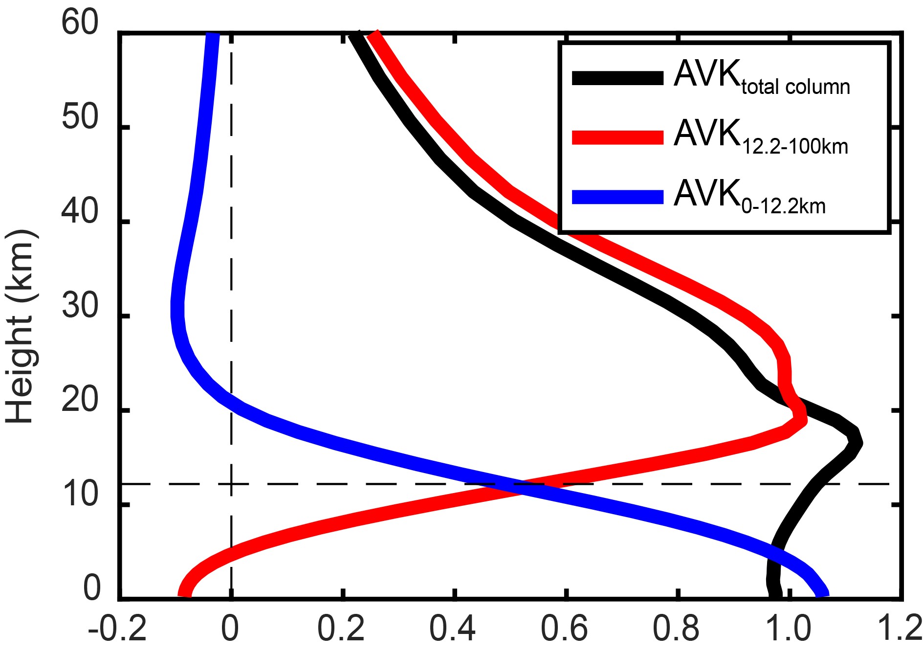 Figure4. Total column averaging kernel (black), together with the partial column averaging kernels of two individual layers (CH4: surface–12.2 km, partial column DOFs=1, and 12.2–60 km, partial column DOFs=1) of one typical NDACC retrieval in Xianghe.
where


Combined in-situ and FTIR measurements provided information about CH4 in three vertical layers: near the ground, in the troposphere, in the stratosphere, and in the total atmospheric column. This enabled us to analyze the temporal and vertical distribution of CH4 in source emission areas.
3
3.2.3. Uncertainty budget
TCCON is a well-developed worldwide observation network. Details of the sources of known uncertainty are described in Wunch et al. (2011). For


For the NDACC observation mode, according to Rodgers (2000), the difference between the true and retrieved state of the atmosphere can be written as follows:
where I is the identity matrix, εb is the error in forward model parameters, and εy is the measurement error. According to Eq. (9), the total error is divided into three error sources: smoothing error, forward model parameter error, and measurement error (Senten et al. 2008). Table 2 shows the values of those errors for a regular observation. In summary, the systematic and random errors of the NDACC total column are about 3.3% and 1.7%, respectively.
| Smoothing error | Measurement error | Forward model parameter error | Total random error | ||
| Interference species error | Temperature (systematic) | Line intensity error (CH4) | |||
| 0.117[%] | 0.104[%] | 0.014[%] | 1.426[%] | 2.938[%] | 1.737[%] |
Table2. CH4 uncertainty budget in NDACC observation mode.
2
3.3. The CarbonTracker-CH4 system
CarbonTracker-CH4 is an assimilation system for atmospheric CH4 developed by the National Oceanic and Atmospheric Administration (NOAA). Using observations from surface stations and towers, CarbonTracker-CH4 assimilates global atmospheric CH4 into TM5 (Transport Model 5; Liu et al., 2016). We used the current release, CT2010, to analyze the atmospheric CH4 mole fractions in Xianghe at the surface. In CarbonTracker-CH4, CH4 emissions into the atmosphere are estimated separately for natural and anthropogenic sources. Natural sources include oceans, wetlands, soil, and insects and wild animals. The anthropogenic sources include emissions from fires, coal, oil and gas production, animals, rice cultivation and waste. We used daily averages from 2010 to determine the contributions from different anthropogenic sources in Xianghe.4.1. Comparison between in-situ and FTIR total column measurements
Figure 5 shows the seasonal variation of CH4 measured by the Picarro G2301 (mole fraction near the ground) and FTIR (total column-averaged dry-air mole fraction of CH4). The means (standard deviation) of the CH4 mole fraction measurements are as follows: 2.2049 ppm (0.0945 ppm) for the Picarro, 1.8839 ppm (0.0129 ppm) for TCCON, and 1.9234 ppm (0.0193 ppm) for NDACC. It is clear that the mole fraction of CH4 near the ground is much higher than the total column-averaged CH4. All three sets of measurements had high values in summer, later autumn, and early winter. A minimum in CH4 in March and April was observed by both in-situ and FTIR measurements. The total columns of CH4 based on the TCCON and NDACC measurements are similar, and the average
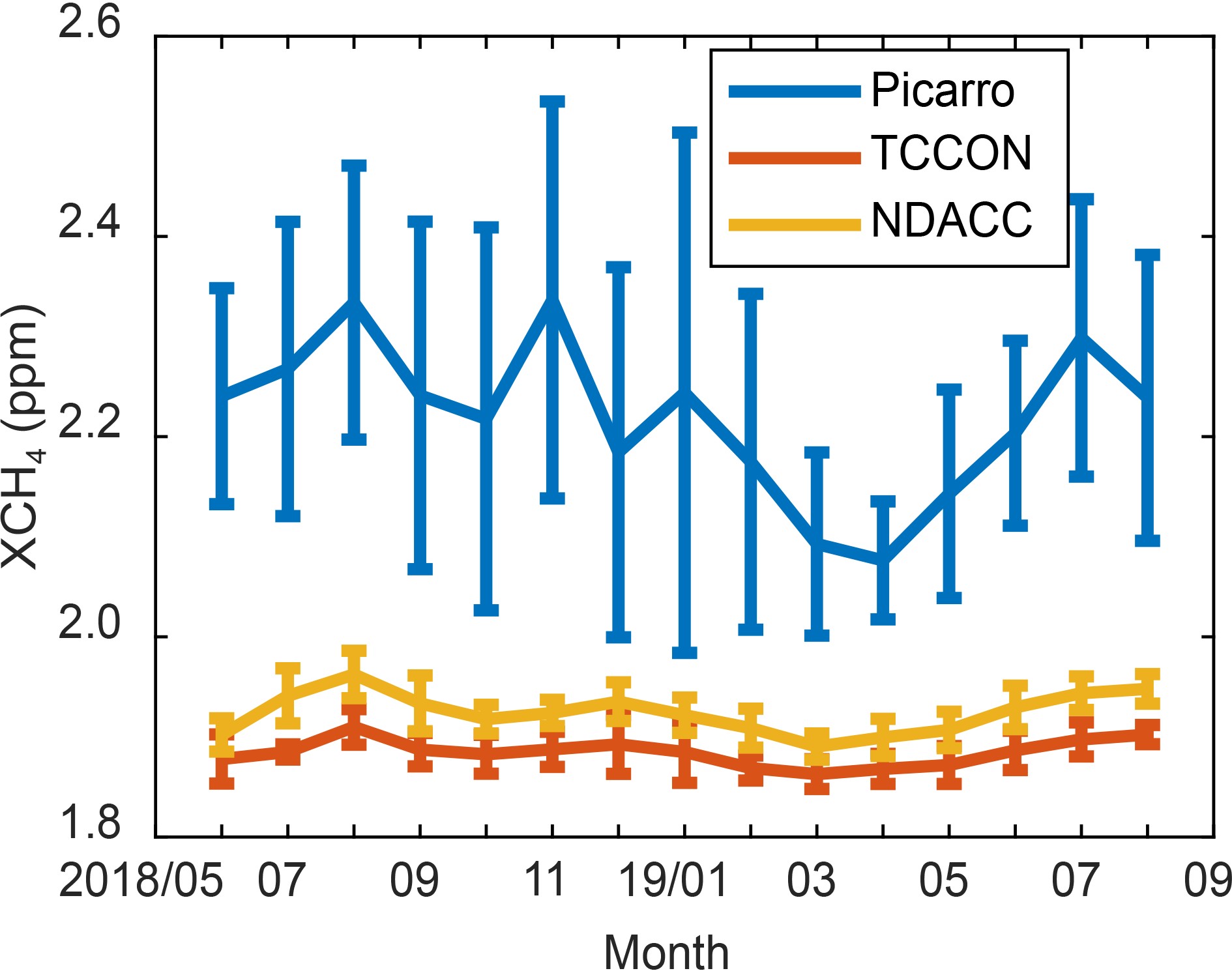 Figure5. Seasonal variation of CH4 measured by Picarro and FTIR. The error bar is 1
Zhang and Qun (2011) analyzed the total column amount of CH4 in China using SCIAMACHY(Scanning Imaging Absorption Spectrometer for Atmospheric Chartography) satellite observations. They found that concentrations of CH4 are higher in summer and lower in winter, which was attributed to biological sources in association with soil temperature and land moisture. The warm and wet soil conditions, leading to higher production in summer, provide a suitable environment for microbes to produce CH4 by anaerobic respiration (Freeman et al., 2002, Hao et al., 2005, He et al., 2019). This is one possible reason for the total column amount of CH4 seen in Xianghe during summer. However, the total column of CH4 in Xianghe in winter was higher than that in spring. These findings indicate that the seasonal variation in total column amounts of CH4 in Xianghe is not fully attributable to biological sources.
2
4.2. Seasonal cycle of CH4 in the troposphere and stratosphere
CH4 varies with altitude, as shown in Fig. 6. In the troposphere, the average CH4 concentration was 2.0599 ± 0.0224 ppm, with two maxima in August and December (2.0977 ± 0.0259 and 2.0608 ± 0.0228 ppm, respectively), and two minima in October and March (2.0387 ± 0.0177 and 2.0196 ± 0.0134 ppm, respectively). Compared with the in-situ measurements at the surface, CH4 is much more well-mixed in the troposphere than near the surface. The variation in the tropospheric column of CH4 is close to that in the in-situ measurements near the ground.In the stratosphere, the annual average CH4 concentration was 1.6498 ± 0.0496 ppm, and was higher in the summer (1.7374 ± 0.0267 ppm) and lower in the winter (1.5700 ± 0.0625 ppm).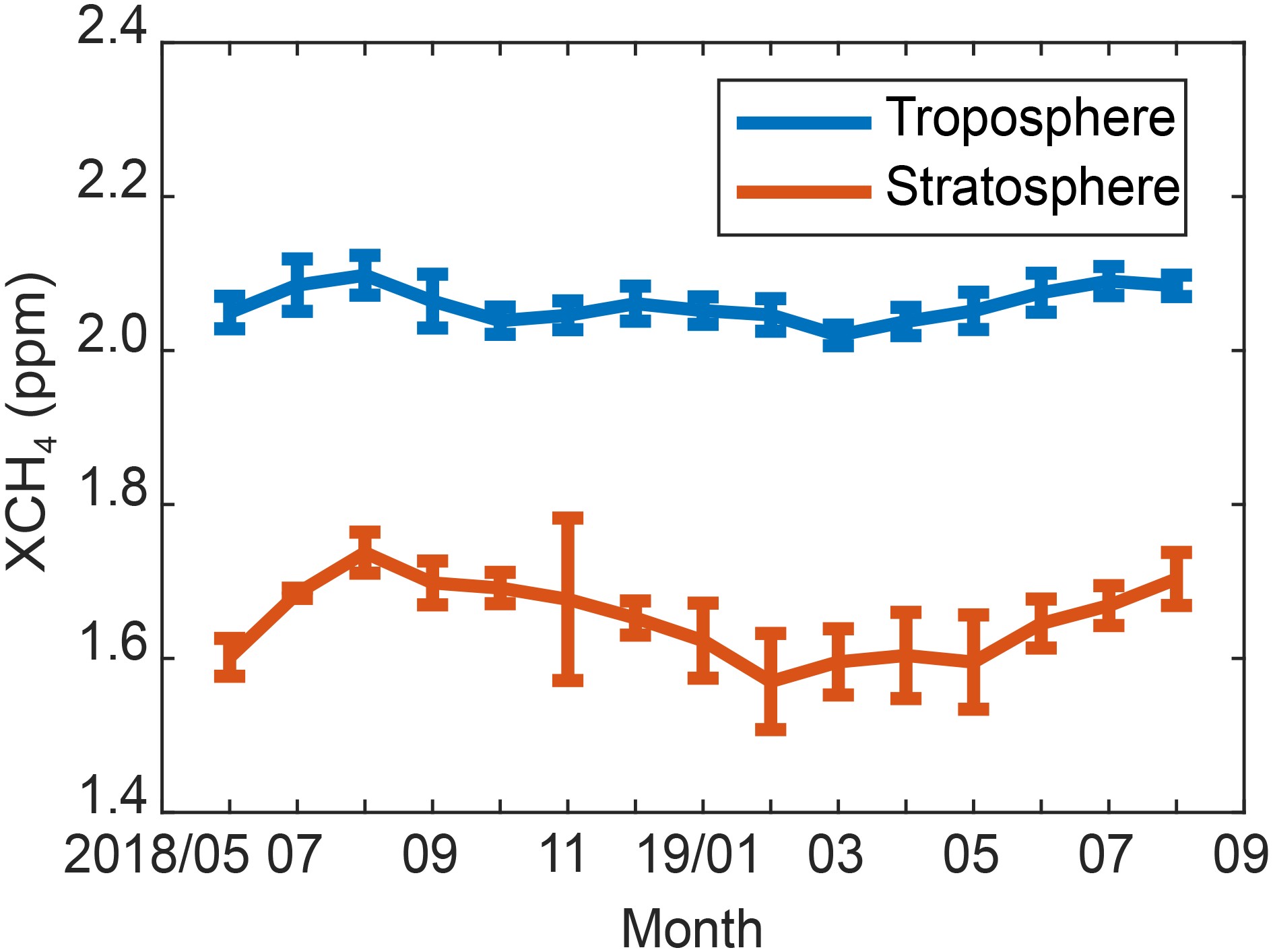 Figure6. Seasonal variations in two different layers: the free troposphere (blue line) and stratosphere (red line). The error bar is 1
Several studies show that the distribution of atmospheric trace gases is related to the Brewer–Dobson circulation (BDC); in midlatitudes, the stratosphere–troposphere exchange (STE) caused by tropopause folding can influence the vertical distribution of long-lived gases, such as CH4, N2O, and O3 (Yang and Lü, 2004; Simmonds et al., 2013; Fan et al., 2014). Simmonds et al. (2013) reported that the BDC is driven by vertically propagating Rossby and gravity waves. When these waves break in the stratosphere, the speed of westerly airflow decreases, which results in high-latitude convergence and the descent of stratospheric air into the troposphere (Lu and Ding, 2013). For detailed characterization of BDC, residual circulation is often used to analyze air mass transport. Many studies have proven that such STE in midlatitudes is dominated by transportation from the stratosphere to the troposphere, which is strong in winter and spring, and weak in summer and autumn (Yang et al., 2003; Simmonds et al., 2013; Fan et al., 2014). Fan et al. (2014) showed that the center of the upwelling residual circulation at 150 hPa tends to shift northwards between April and August, and southwards between September and February of the following year. More specifically, this upwelling center can be situated at 40°N in the summer, which is very close to the study region of Xianghe. Therefore, the CH4 measurements in Xianghe could provide information about CH4 transport between the stratosphere and troposphere.
Figure 7 shows the annual-averaged


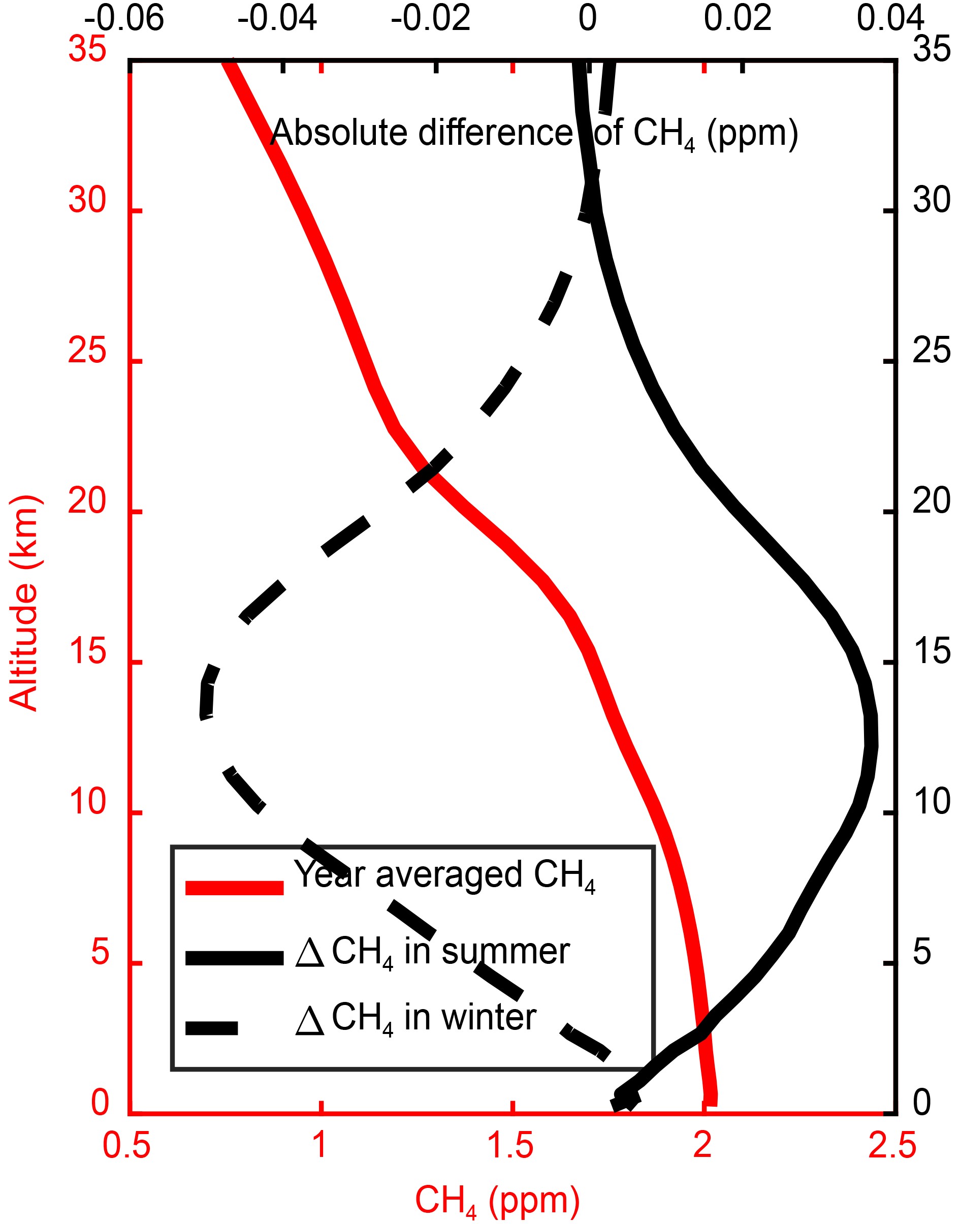 Figure7. The yearly averaged profile of CH4 in Xianghe (red line), and the profile of the difference between the mean CH4 profile in summer with the yearly averaged one (black solid line), and the profile of the difference between the mean CH4 profile in winter with the yearly averaged one (black dashed line).
In summary, we found that CH4 in the troposphere was relatively well-mixed, with little variation. There were two peaks: one in the summer, caused by local sources of CH4, and one in winter, resulting from fewer hydroxyl radicals. In the stratosphere, the mixing ratio of CH4 could be influenced by the STE, which reaches a maximum in summer and a minimum in winter.
2
4.3. Diurnal variation of CH4 near the ground
We mainly attribute the diurnal changes in the CH4 mole fraction to three factors: local source emissions, diurnal variation of the boundary layer (which could impact the dilution of CH4), and the rate of oxidation by OH free-radicals (Fang et al., 2012). At most background stations, the CH4 mole fraction is lower during the daytime than at night, since transport and photochemical sinks are more influential during the day (Fang et al., 2012). However, in some source areas, such as rice paddies, CH4 emission flux increases with temperature during the daytime, reaching a maximum value at 1500LT. Thereafter, the CH4 flux decreases with temperature (Lu et al., 2015).It is obvious that, in source areas, the diurnal variation of CH4 is mostly influenced by local emissions. Xianghe is a typical source area; diurnal variation of CH4 from in-situ measurements at this site are shown in Fig. 8. In spring, summer, and autumn, the CH4 mole fraction was higher at night (1800–0600 LT) than during the daytime (0600–1800 LT); it grows slowly but continuously, peaking at 2300 LT, before decreasing rapidly until 0600 LT the next day. However, in winter, there was no apparent difference in the CH4 mole fraction between daytime and nighttime; it increased between 0600 and 1500 LT and was stable between 1500 and 2400 LT, after which it decreased as in all other seasons.
 Figure8. Diurnal variation of CH4 at the surface from spring to winter. The time units are in local time (+8 h UTC). The error bar is 1
Recall that there are three factors that may affect the diurnal variation of CH4 at the surface. First, OH free-radical oxidation is a relatively slow process during the day, having a rate of 360 × 1012–530 × 1012 gyr?1 (about 0.179 ppm yr?1); this cannot explain the observed dramatic change in CH4 (Wang, 1991). Aside from during the winter, the inflexion points of the CH4 signal occurred in the morning (~0600 LT) and afternoon (~1600–1700 LT). Assuming strong CH4 emissions at the surface, concentrations are diluted in the deeper daytime boundary layer, whereas at nighttime CH4 accumulates in the shallower boundary layer. This results in the CH4 mole fraction during the daytime being lower than at night, thus showing the influence of the boundary layer on the diurnal variations of CH4.
Some studies show that the diurnal variation of emissions from landfill waste is greater at night than during the daytime (B?rjesson and Svensson, 1997; Chen et al., 2008). In winter, the inflexion point was in the afternoon (~1500 LT), which is relatively different than for the other seasons. This difference may be a result of strong anthropogenic emissions at the surface close to Xianghe.
The Beijing–Tianjin–Hebei region is dominated by domestic landfill waste and wastewater treatment (Le et al., 2012; Huang et al., 2019). Huang et al. (2019) found that CH4 emissions from domestic landfill waste and wastewater treatment accounts for more than 30% of total CH4 emissions in Beijing and Tianjin. However, the proportion of arable land in the Beijing–Tianjin–Hebei region gradually decreased between 1990 and 2015, by about 50% (Gong et al., 2019). Therefore, CH4 emission sources may have changed as arable land availability decreased, and as wastewater and domestic garbage treatment increased. Also, in 2018, a new domestic waste site was created about 8 km away from the Xianghe site. We deduce that CH4 emissions in Xianghe are most likely related to domestic landfill waste and wastewater treatment. Further investigation is needed to understand the diurnal variation of emissions, which in turn could help us to better understand the diurnal variation of CH4 in particular.
2
4.4. CarbonTracker-CH4 model simulations
We used CarbonTracker model simulations to analyze emission contributions from different sources in Xianghe. Figure 9a shows the seasonal variation of the CH4 mole fraction in 2010 from six different sources: fossil fuels; insects/wild animals; rice cultivation and waste; wetlands and soil; oceans; and wildfires. Fossil fuels, wildfires, and oceans are not as important as the other sources, only accounting for about 15% of total emissions in Xianghe. The most important sources are animals, rice cultivation, and waste, which accounted for about 32.6% of the total emissions.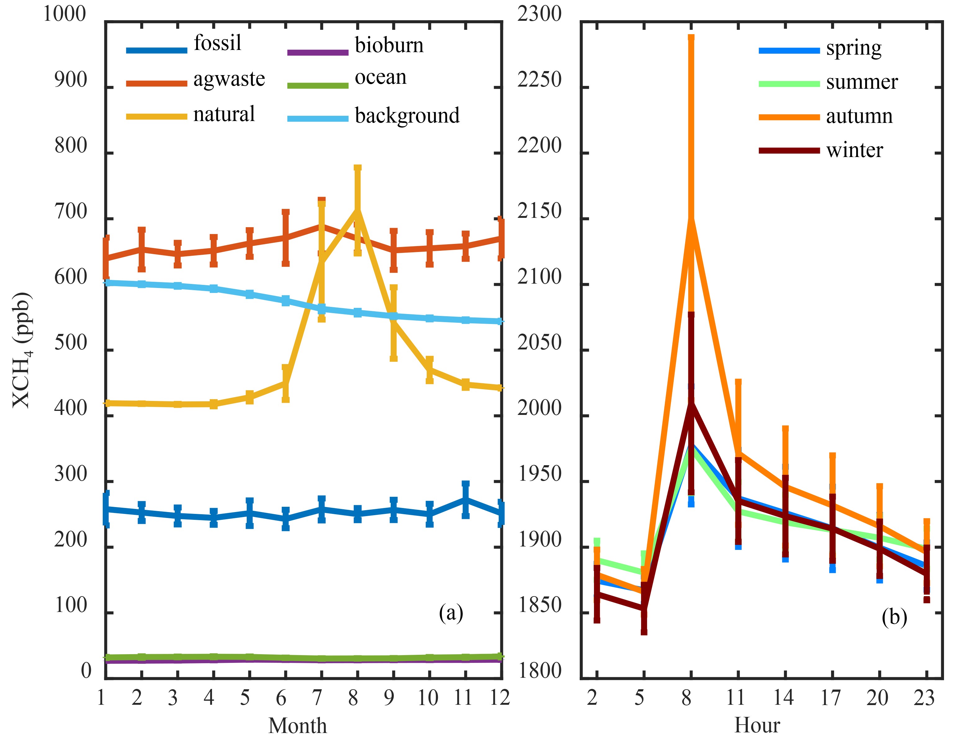 Figure9. Model results of (a) seasonal variation of the mean and standard deviation of CH4 mole fraction near the surface due to different sources, wherein the dark blue line represents emissions from fossil fuels, the red line represents emissions from animals, rice cultivation and waste, the yellow line represents natural emissions from wetlands, soil, oceans and insects/wild animals, the purple line represents emissions from the oceans, and the light blue line represents emissions from fires. The error bar is 1

The largest seasonal variation in emissions was found for wetlands, soil, oceans, and insects/wild animals; emissions were higher in the summer (~700 ppb in August) and lower in other seasons (~420 ppb). This helps explain the relatively high values measured in-situ, especially in August. A small peak in December for agriculture waste was simulated, which may explain the measured peak of the CH4 mole fraction near the surface at this time.
According to the modeled diurnal variation of the CH4 mole fraction (Fig. 9b), maximum values occurred every day at 0800 LT from spring to winter; this was not shown by the in-situ measurements. Since the model simulation was for 2010 (about nine years ago at the time of writing), sources of CH4 may have changed greatly, especially with regard to domestic landfill waste and wastewater treatment, which has recently played a more important role.
The mean (standard deviation) of the CH4 mole fraction near the ground measured by the Picarro instrument was 2.2049 ppm (0.0945 ppm). The mean (standard deviation)


The CH4 mole fraction near the ground reached its maximum value near midnight (~2200–2300 LT), with its minimum value occurring at 0600–0700 LT. The daily maximum values in summer were relatively higher than in other seasons, at nearly 2.4 ppm.
Comparing CarbonTracker-CH4 model simulations with our observations near the ground in Xianghe, we found that the model can reproduce the peak value of the CH4 mole fraction in summer, but underestimates the peak value in winter. The modeled and measured daily variation of the CH4 mole fraction differed.
In summary, we analyzed the temporal and vertical distributions of CH4 in source emission areas using Picarro and FTIR measurements. The vertical distributions could be very useful for understanding the source emissions at such a polluted site.
Acknowledgements. This research was funded by the National Key R&D Program of China (Grant Nos. 2017YFB0504000 and 2017YFC150 1701) and the National Natural Science Foundation of China (Grant No. 41975035). We want to thank the TCCON community for sharing the GGG2014 retrieval code, the NDACC community for sharing the SFIT4 retrieval code, and NOAA for providing the CarbonTracker-CH4 Data Assimilation Product. We also want to thank Weidong NAN, Qing YAO, and Qun CHEN (Xianghe site) for the maintenance of the in-situ and FTIR measurements at Xianghe.
