HTML
--> --> -->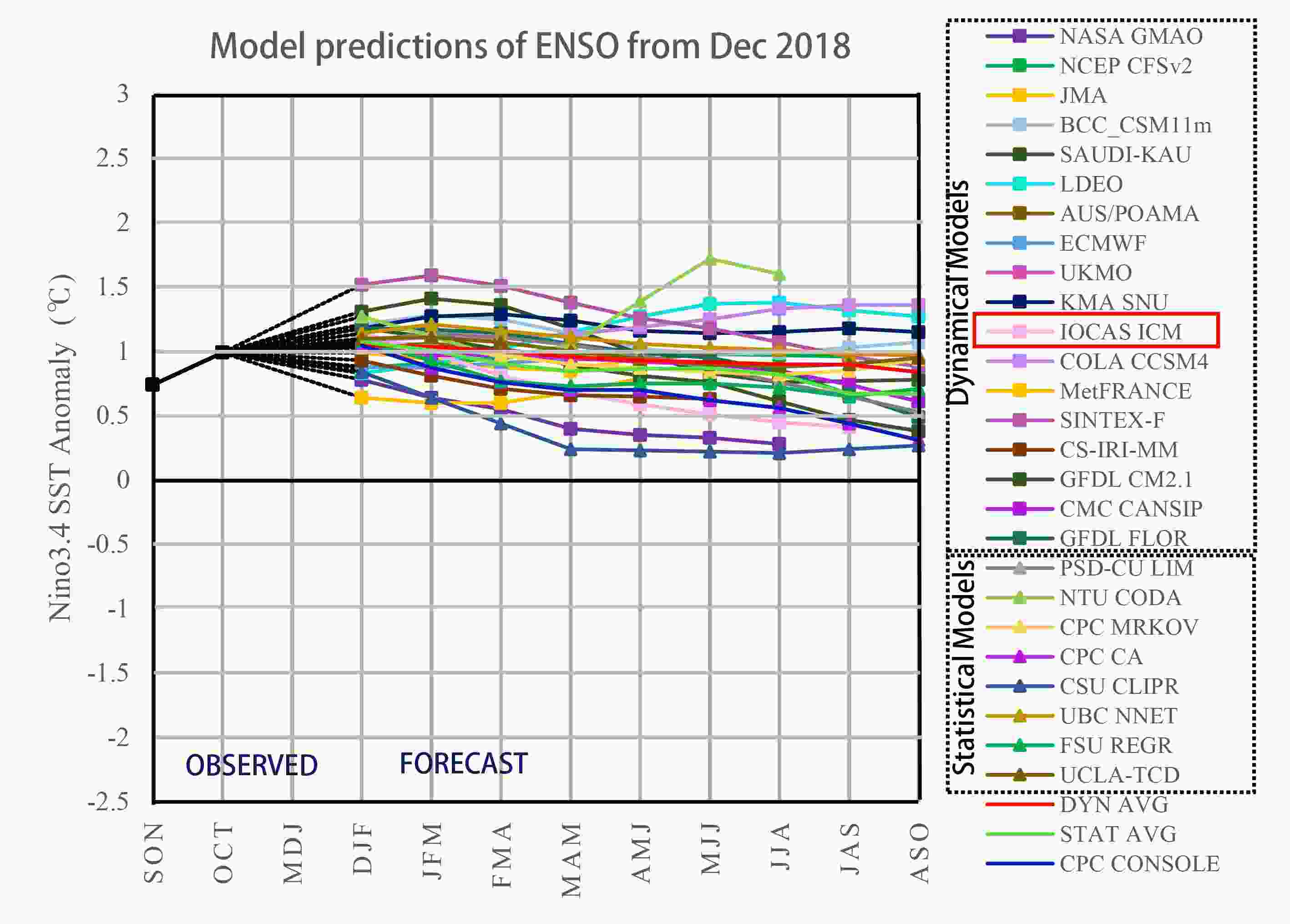 Figure1. Dynamic and statistical models for real-time ENSO prediction from the IRI website, including IOCAS ICM (red rectangle).
Actually, significant uncertainties exist in ENSO forecasts; these uncertainties are mainly from defective initial conditions and imperfect representations of the model dynamics process. In particular, studies have shown that initial conditions can influence ENSO forecasts (Rosati et al., 1997; Fan et al., 2000; Lee et al., 2018). Recently, many researchers have focused on improving the initial conditions of ENSO prediction. Gao et al. (2016) optimized the initial conditions of an improved intermediate coupled model (ICM) using a four-dimensional variational data assimilation (4D-VAR) method to improve ENSO prediction. Tao et al. (2017) examined the initial-error-induced optimal perturbation of ENSO predictions in an ICM. Zhang et al. (2018) improved the simulations of the 2015 El Ni?o event by applying error correction to the initial conditions and model parameters in the ICM. Tao et al. (2018) showed that ENSO prediction errors can be reduced by 25% when the initial-condition errors are removed in the central equatorial Pacific. Gao et al. (2018) optimized the model parameters and initial conditions together through the 4D-VAR method for ENSO studies in an ICM. In fact, the initial perturbation, which can develop into a weather or climate event, can act as the optimal precursor (OPR) for the weather or climate event. Therefore, the OPR of ENSO can be represented by the initial perturbation that most likely evolves into an ENSO event. Obtaining the OPR of ENSO can help to find the early signal that will evolve into an ENSO event and indicate the evolutionary process of the ENSO event (Mu et al., 2014).
Some studies on the OPR of ENSO have already been conducted. Duan et al. (2004) investigated OPRs for ENSO events with a theoretical coupled oceanЈCatmosphere model, and discussed the physical mechanism of the OPRs for ENSO. Duan et al. (2013) explored the manner in which nonlinearities modulate El Ni?o events by investigating the optimal precursory disturbance for El Ni?o events in the Zebiak?Cane (ZC) model. Mu et al. (2014) revealed the great similarity between the OPR and the optimally growing initial errors in terms of localization and spatial structure using the ZC model. Capotondi and Sardeshmukh (2015) investigated the OPRs of different ENSO events based on a linear inverse modeling framework using observational SSTs and thermocline depth data and concluded that the predictability of different types of ENSO events depends mainly on the initial subsurface conditions. Hu and Duan (2016) found that the optimal precursory disturbance for La Ni?a is almost opposite to that of El Ni?o, using the Community Earth System Model (CESM).
However, whether the OPRs in different models show the same spatial structure is still worthy of study. In addition, how to obtain the OPRs is a mathematical problem. Currently, many methods, including methods with linear assumptions and nonlinear methods, have been proposed and can be used to obtain the OPR, a special initial perturbation. Those methods with linear assumptions are limited when the nonlinear effect is nonignorable because the evolution of the ENSO event is largely a significant nonlinear one. Hence, it is more reasonable to adopt a nonlinear method, and the conditional nonlinear optimal perturbation (CNOP) method is an effective nonlinear method for studying the predictability of the ENSO phenomenon.
The CNOP method, which was proposed by Mu and Duan (2003) to study the predictability of ENSO, is an extension of the singular vector in a nonlinear regime and can represent the initial perturbation (or the OPR) that will trigger the ENSO event. Various methods have been proposed to solve the CNOP, including the adjoint method, intelligent algorithms (Mu et al., 2015; Ren et al., 2016), ensemble projection algorithms (Wang and Tan, 2010; Chen et al., 2015) and the gradient-definition-based method (GD method) (Mu et al., 2017, 2019). The adjoint method is strongly dependent on the adjoint models, which are developed using adjoint technology and take large amounts of time and energy to develop and verify (Gao et al., 2016), but some models or modules still have no corresponding adjoint models or modules (Mu et al., 2019). Intelligent algorithms solve the CNOP by searching the solution space randomly, so a certain randomness is unavoidable (Mu et al., 2015; Ren et al., 2016). Ensemble projection algorithms introduce the experience value, which is not always reliable. The GD method, which was first proposed to solve the CNOP by Mu et al. (2017), can avoid using adjoint models. This method has been applied to solve the CNOP in the ZC (Mu et al., 2017) and MM5 (Mu et al., 2019) models and has been proven to be an effective method to solve the CNOP. However, whether the GD method works for all models deserves further study.
In this paper, the GD method is adopted to seek the CNOP to depict the optimal SST precursors (SST-OPRs) of ENSO events in the IOCAS (Institute of Oceanology, Chinese Academy of Sciences) ICM. Non-El Ni?o events simulated by the ICM are chosen as the basic events to represent the OPR of ENSO, and the SST-OPRs for different initial months of those events are calculated using the GD method. Experimental results show that the GD method is an effective way to obtain the SST-OPRs of ENSO events, and the obtained SST-OPRs indicate positive SSTA signals in the western-central equatorial Pacific. However, the patterns along the equator are completely different and show a certain seasonal dependence. Further experiments illustrate that the non-El Ni?o events can eventually evolve into El Ni?o events when the seasonal SST-OPRs are superimposed on the corresponding seasons, and the peaks of the Ni?o3.4 index for those events occur at the end of the years, which is consistent with the evolution of the real El Ni?o events.
The rest of this paper is organized as follows. Section 2 describes the IOCAS ICM model, the CNOP and the GD method. Section 3 shows the experimental setup and parameter determination in detail. The experimental results and related analysis are shown in section 4. Finally, concluding remarks and discussion are given in section 5.
2.1. IOCAS ICM
The IOCAS ICM was developed by Zhang et al. (2003) to simulate and predict SST variability in the tropical Pacific. The ICM has already been successfully used for ENSO simulations and predictions (Zhang and Gao, 2016b; Gao and Zhang, 2017). Moreover, it has also been used to perform routine real-time ENSO forecasts whose results are posted at the IRI website for Climate and Society.IOCAS ICM consists of a dynamic ocean model and an empirical atmospheric model, as shown in Fig. 2. The dynamic ocean model is based on an intermediate ocean model (IOM) developed by Keenlyside and Kleeman (2002), an SSTA model and an empirical representation of water temperature entrained into the mixed layer, Te (Te model). The empirical atmospheric model is a statistical model (Іг model), which takes the empirical feedback response of the wind stress (Іг) to SSTAs into account. Figure 2 also illustrates the coupling relationship between the IOM, SSTA model, Te model and Іг model. Specifically, at each time step, the IOM produces the oceanic horizontal and vertical advections and the oceanic pressure field (including sea surface pressure anomalies). The Te anomalies are then estimated based on the oceanic pressure field by the Te model (Zhang and Gao, 2016a). The horizontal and vertical advections produced in the IOM, the Te anomalies produced by the Te model, the prescribed climatology of the mean currents and so forth are passed to the SST model to calculate the SSTAs. Then, the calculated SSTAs are passed to the Іг model to calculate the wind stress anomalies, which are used to force the IOM. In addition, the ICM is initialized with the imposed westerly wind anomaly for eight months. The evolution of anomalous conditions thereafter is then determined solely by the coupled ocean?atmosphere interactions in the ICM described above. More details of the IOM can be found in Keenlyside (2001) and Keenlyside and Kleeman (2002), and details of the Te model, SSTA model and Іг model can be found in Zhang and Gao (2016b).
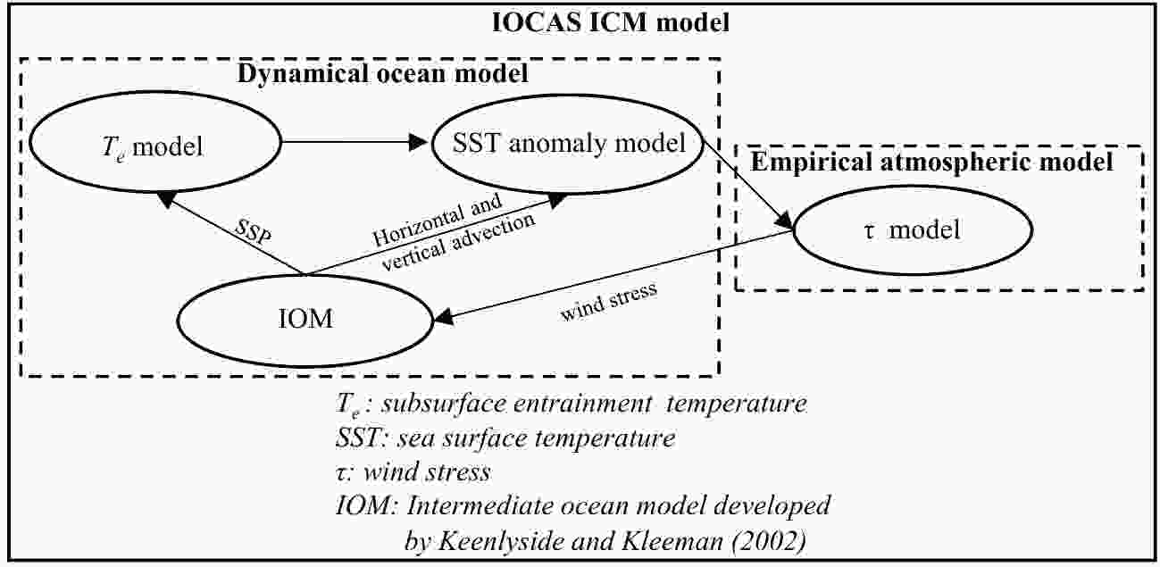 Figure2. Components involved in IOCAS ICM and the coupling relationship between them.
2
2.2. CNOP method
In this paper, the CNOP method proposed by Mu and Duan (2003) is chosen to study the OPRs of ENSO events in the ICM. The CNOP can represent the initial perturbation, which can lead to the largest nonlinear evolution at the prediction time. The OPR of ENSO can be regarded as a kind of CNOP that will evolve into an ENSO event at the prediction time. To solve the SST-OPRs, suppose we have the following ICM:where Micm is the integral operator of the ICM, S0 is the state at the initial integration time and Sf is the state at the end of the integration time. Both S0 and Sf are n-dimensional state vectors.
It is known that the CNOP is a kind of initial error added to the initial state. Suppose p is the initial error added to the initial state S0; then, the development of the initial error p can be described as follows:
where p is the so-called initial perturbation and Sp is the state at the end of the integration time when the initial error p is added. According to the definition, the CNOP can be solved by the following maximum optimization problem:
where

Therefore, the CNOP can be obtained by solving the optimization problem in Eq. (4). The objective function of this problem can be described by


2
2.3. GD method
As mentioned above, the GD method was first proposed to solve the CNOP by Mu et al. (2017). It has been applied to solve the CNOP in the MM5 and ZC models and has been proven to be an effective method to solve the CNOP (Mu et al., 2017, 2019). According to the optimization problem in Eq. (4), the adaptive function for solving the CNOP has the following form:The main idea of the GD method is to calculate the gradient by the gradient definition in mathematics and then to solve the optimization problem using the SPG2 algorithm. In fact,

where F Ёф(p) and f Ёф(p) are the partial derivatives of F(p) and f(p), respectively. Suppose that the initial perturbation

where


where Іи is a positive real number that approaches 0 but never equals 0; pІи represents the initial error


2
2.4. Dimension-reduction-based singular value decomposition
As mentioned in section 2.1, the resolution of SSTAs is 134 ЁС 61 (= 8174), so the original solving space is 8174-dimensional for the optimization problem in Eq. (4). It is a high dimension for solving the CNOP using the GD method. To improve the time efficiency, dimension reduction is carried out, and the singular value decomposition (SVD) method is adopted to reduce the dimension of the solution space. Two steps are performed to conduct the dimension reduction: the first is to generate samples, and the second is to perform the eigen-decomposition using the SVD method.It is known that the ICM is an anomaly model in which the SSTA is directly produced by the ICM. To obtain the samples, the ICM is integrated for 200 years, and the monthly SSTAs are collected as the samples, totaling 200 ЁС 12 = 2400. However, the first 80 years are the adjustment stage for the ICM, so samples for the first 80 years are abandoned to obtain reliable samples; 120 ЁС 12 = 1440 samples are collected as the final matrix. After the sample matrix is determined, the SVD method is applied to perform the eigen-decomposition for the sample matrix using the following function provided by Matlab 2010:
where As represents the sample matrix, in which every column is a sample and the number of the samples (1440) is the number of rows of the matrix. Therefore, As is an 8174 ЁС 1440 matrix. U is a 8174 ЁС 8174 matrix composed of the eigenvector of the matrix As AsT, S is a 8174 ЁС 1440 eigenvalue matrix, and V is a 1440 ЁС 1440 matrix composed of the eigenvector of the matrix AsTAs, in which the matrix AsT is the transposed matrix of As. The matrix U can represent the feature space in which the samples lie. The eigenvectors are sorted in descending order of the corresponding eigenvalues, so the matrix UЁф composed of the first m (m?8174) eigenvectors can produce a new low-dimensional space representing the original solving space. Thus, the dimension of the original space can be reduced.
Although the solving space can be reduced using the SVD method, it is not possible to run IOCAS ICM in the feature space, because every variable has its own physical meaning. So, the variables need to be converted from the feature space to the original space when running IOCAS ICM. This is done using the eigenvector matrix.
3.1. Experimental setup
In this paper, IOCAS ICM is chosen to study the SST-OPR of ENSO. The spatial domain of the IOM extends from 31ЁуS to 31ЁуN and from 124ЁуE to 30ЁуE, which covers the tropical Pacific and Atlantic basins. For convenience, only the SSTAs in the region from 31ЁуS to 31ЁуN and from 124ЁуE to 70ЁуW are shown in the following experiments. The region for SSTAs is divided into 134 ЁС 61 grid points for the sea surface. In addition, the CNOP and OPR are solved using the GD method in the ICM and coded using Fortran on the Linux platform.To seek the SST-OPR of ENSO in the ICM, the non-ENSO years simulated by the ICM are selected as the basic years. Figure 3 shows the temporal evolution of the Ni?o3.4 index for the three chosen continuous basic years simulated by the ICM. For convenience, the first year is denoted by year(1), the second year by year(2), and so on. The CNOPs for the initial months from July(1) of year(1) to June(3) of year(3) are calculated; these months are shown between the two dashed lines in Fig. 3. Therefore, a total of 24 CNOPs can be obtained with a lead time of 12 months (one year).
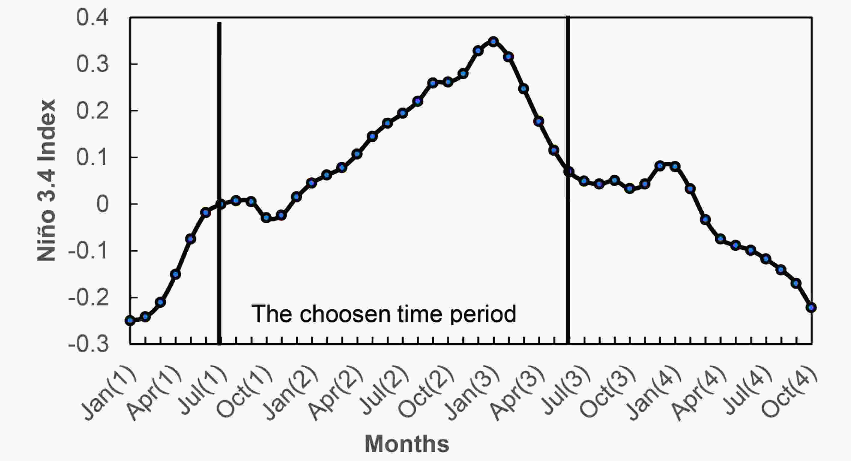 Figure3. Temporal evolution of the Ni?o3.4 index for the chosen basic years. The months between the black lines are the chosen time period to study the OPRs of ENSO.
Considering the seasonal dependence of the CNOPs in the later experiments, the calendar year is divided into four seasons, from January to March (JFM), April to June (AMJ), and then JAS and OND. In addition, to improve the time efficiency, the MPI parallel strategy is adopted to accelerate the way the CNOPs are solved. All experiments are run on a Tinahe-2 supercomputer system at the National Supercomputer Center in Guangzhou, China, in which each node has two Intel(R) Xeon(R) CPU E5-2692v2 @ 2.20 GHz physical CPUs; each CPU has 12 logical cores, for a total of 24 processors for each node.
2
3.2. Parameter determinations
When solving the OPR of ENSO, many parameters are involved. The three crucial parameters are the dimension of the feature space (DoF), the constraint for the initial perturbation ІФ in Eq. (3) and the value of Іи in Eq. (8), which are discussed in this section.The DoF is determined by the number of features that are decided after performing the SVD analysis. Figure 4 illustrates the change of the eigenvalue and the cumulative eigenvalue ratio with an increasing number of eigenvectors. From Fig. 4, the accumulated eigenvalue ratio increases with increasing eigenvectors, and the ratio reaches more than 95% when the eigenvectors are more than 48. After that, the curve of the ratio tends to become gentler; that is, the ratio changes very slowly. Considering that more features will require more time, it has been found that the adaptive function value and the CNOP pattern obtained do not change much when more features are included. Therefore, the DoF is set to 48 for the subsequent experiments.
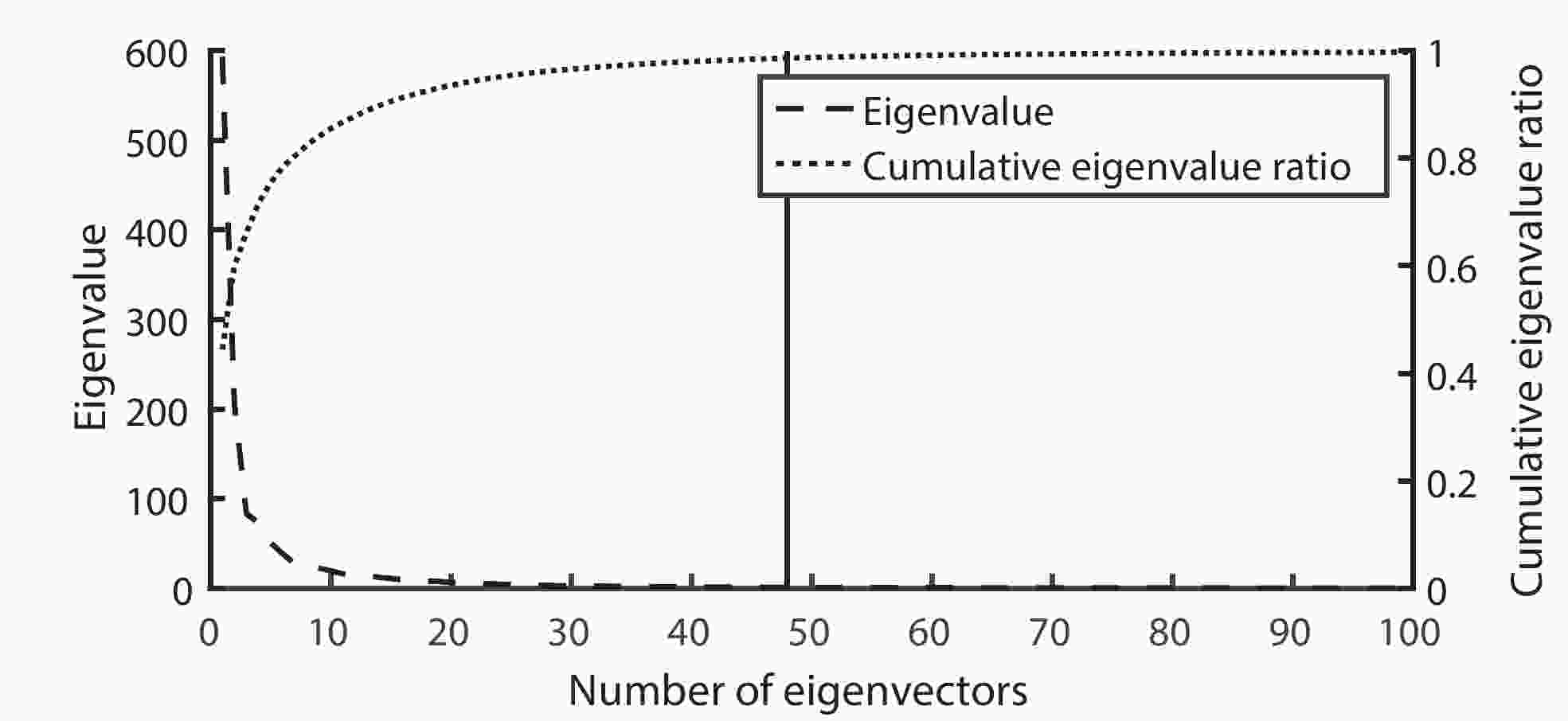 Figure4. Corresponding eigenvalue and cumulative eigenvalue ratio for the first 100 eigenvectors.
The constraint for the initial perturbation ІФ in Eq. (3) is also a crucial parameter in this study. It is obvious that the larger the ІФ is, the larger the objective function value. (A larger objective function value means that the SSTA added to the initial state is larger.) However, the SSTA in a real scenario cannot be infinite. Therefore, it is necessary to determine a suitable constraint for the initial perturbation. Here, we adopt the objective function value mentioned in section 2.2 and the average SSTA in the Ni?o3.4 areas to show the size of the CNOP for different ІФ values when the initial month is January and the lead time is nine months. Figure 5 shows the change in the objective function value and the SSTA in the Ni?o3.4 areas (5ЁуS?5ЁуN, 170ЁуE?120ЁуW) as ІФ changes. From Fig. 5, the objective function value and the SSTA in the Ni?o3.4 areas increase with increasing ІФ, and the increasing trend for the SSTA in the Ni?o3.4 areas decreases when the ІФ is larger than 10. According to the definition of the National Oceanic and Atmospheric Administration (NOAA) in 2003, an El Ni?o event can be confirmed to occur if the SSTAs of a three-month running mean in the Ni?o3.4 index are above 0.5ЁуC for more than three months. Therefore, the initial SST perturbation should be chosen as no more than 0.5ЁуC, and less than 10% of 0.5ЁуC (0.05ЁуC) can be the constraint of the initial SSTA based on experience. From Fig. 5, the average SSTA in the Ni?o3.4 areas is 0.042 (< 0.05ЁуC) when the ІФ is set to 10. Therefore, the constraint ІФ is set to 10 in this study.
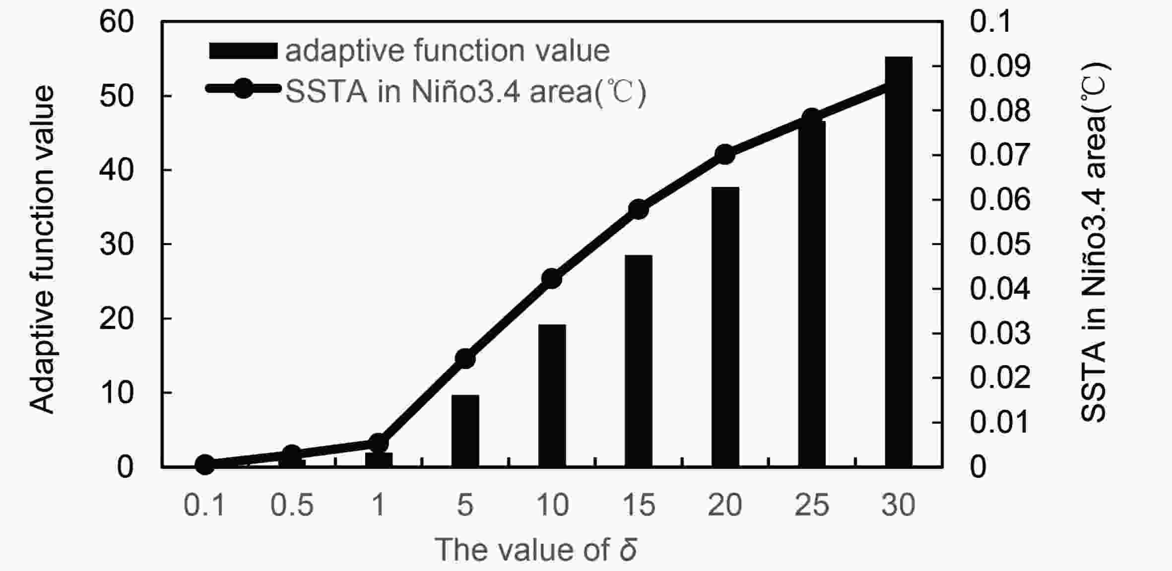 Figure5. Objective function value and SSTA in Ni?o3.4 areas for different ІФ.
In Eq. (8), Іи is another crucial parameter when calculating the gradient using the limit in mathematics. In this situation, Іи should be a positive real number that should approach 0 but never equal 0. Considering that the evolution


The parameters used in the experiments are listed in Table 1. Additionally, other parameters that can be determined according to usersЁЏ own requirements are also shown in Table 1, such as the maximum iterations in the SPG2 algorithm and the lead time when solving the CNOP for the ICM.
| Parameters | Value | Meaning |
| DoF | 48 | Dimension of the feature space |
| ІФ | 10 | Constraint of the initial perturbation |
| maxit | 50 | Maximum iterations in the SPG2 algorithm |
| Lt(months) | 9 | Lead time when solving the CNOP for the ICM |
| Іи | $0.01\sqrt {\dfrac{{{\delta ^2}}}{{{\rm{DoF}}}}} $ | A parameter in Eq. (10) |
Table1. Parameters involved in this study.
4.1. The CNOP magnitude
To investigate the magnitude of the CNOPs, the CNOPs for the initial months from July in year(1) to June in year(3) are obtained by solving the optimization problem described in Eq. (4) with a lead time of 12 months. Then, the ЁАbasic runЁБ and the ЁАCNOP runЁБ are carried out to calculate the corresponding objective function value to investigate the magnitude of the CNOPs. The basic run or ЁАnature runЁБ involves running the ICM starting from the initial basic state to the end time of prediction, while the CNOP run involves running the ICM by superimposing CNOP-type errors on the corresponding initial basic states from the basic run. This process is demonstrated in Fig. 6. Then, the objective function value can be calculated using the equation of the objective function described in section 2.2.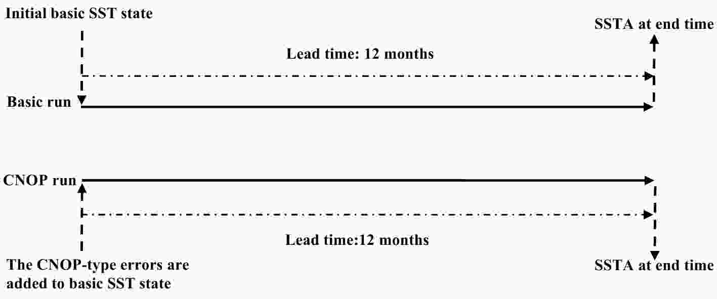 Figure6. Schematic diagram for evaluating the magnitude of the CNOPs.
Figure 7 shows the objective function values of CNOPs for different months from July in year(1) to June in year(3). From Fig. 7, the objective function values of CNOPs for different seasons are quite different, with seasonal changes. The largest objective function values can always be reached when the initial months are in the JFM season, which can be explained by the fact that ENSO events always tend to have a peak in winter (JFM). The smallest values are observed when the initial months are in the JAS season. Therefore, it can be implied that the objective function values of the CNOPs for different initial months exhibit particular uncertainty and are sensitive to the seasons.
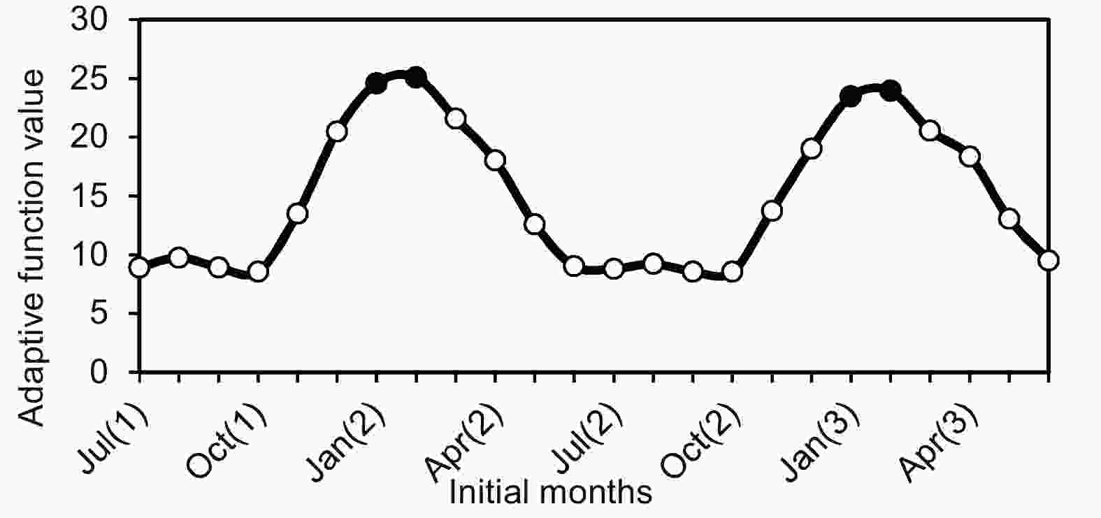 Figure7. Objective function value of the CNOPs for different months from July in year(1) to June in year(3).
2
4.2. The CNOP pattern
As mentioned in section 4.1, 24 CNOPs can be obtained for different initial months from July in year(1) to June in year(3). By investigating their spatial structures, it is found that the patterns for those CNOPs show a certain seasonal dependence; that is, the patterns of CNOPs with the same start season are quite similar. Figure 8 shows the spatial structures of CNOPs for different seasons. It can be seen that all the CNOPs present positive SSTA signals in the western-central equatorial Pacific, but the patterns for different seasonal CNOPs exhibit obvious differences along the western-central equatorial Pacific. The details are presented as follows.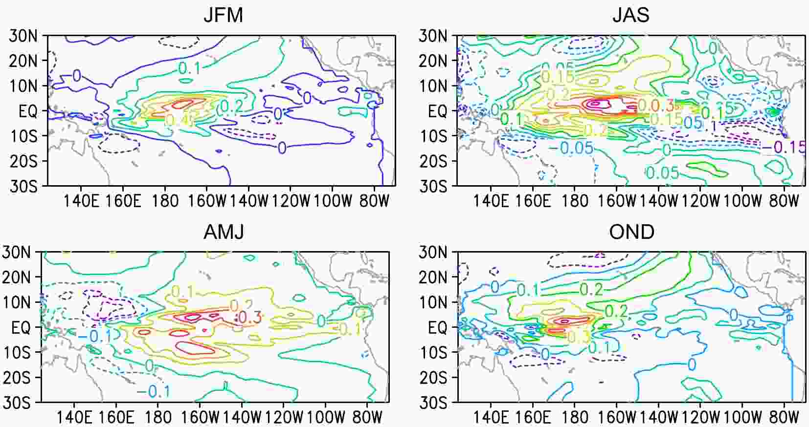 Figure8. Spatial structures of optimal SST precursors for different seasons. Only the SST precursors for March, June, September and December are shown here because the CNOP patterns for the same start season are quite similar.
Overall, the four seasonal CNOPs clearly show positive anomaly signals near the dateline in the equatorial Pacific, but their patterns off the equator are completely different. For the JFM (winter) season, the pattern of the CNOPs presents a dipole structure along the equator, while the positive anomaly area lies in the central-western Pacific and the negative anomaly area lies in the southern equatorial central Pacific. For the JAS (summer) season, the spatial pattern also shows a dipole structure similar to that of the JFM season, but the area with a positive anomaly shows a larger-scale distribution in the central equatorial Pacific, which almost covers the Ni?o3 and Ni?o4 areas. In contrast, the negative anomaly area lies in the southeastern equatorial Pacific, an area with a larger value than that of the JFM season and smaller value than the positive anomaly. For the AMJ (spring) and OND (autumn) seasons, their main patterns both show positive anomaly areas along the equator. Specifically, the positive anomaly area is around the dateline in the central equatorial Pacific for the AMJ season, while for the OND season the positive anomaly area lies west of the dateline in the equatorial Pacific.
In addition, similar results were reported by Tao et al. (2017), in which the seasonal CNOPs were also obtained. The basic events were ENSO events in their work, while the basic events in this paper are non-ENSO events; therefore, the CNOP patterns are not the same. Nonetheless, both show that the CNOP shows certain seasonal dependence.
2
4.3. Temporal evolution of the Ni?o3.4 index
The magnitude and spatial structure of the CNOPs have been investigated in sections 4.1 and 4.2. However, whether the CNOPs can represent the SST-OPRs of the ENSO events has still not been discussed, and the way to identify the SST-OPRs is to investigate the Ni?o3.4 index according to the definition of an El Ni?o event by the NOAA in 2003. Therefore, the 24 CNOPs mentioned in section 4.2 are superimposed on the corresponding 24 basic initial months to gain the temporal evolution of the Ni?o3.4 index, and the results are shown in Fig. 9. Figure9. Temporal evolution of Ni?o3.4 index when the SST-OPRs are added to the responding initial months. The black curve is the initial Ni?o3.4 index. The evolutions of the Ni?o3.4 index starting from the initial months of the OPRs are added, e.g., July(1) means the Ni?o3.4 index starts from July in year(1). The red and green dotted lines represent January(3) and January(4) respectively; that is, the peaks of the Ni?o3.4 index. The black dashed lines represent 0.5Ёц and ?0.5Ёц.
From Fig. 9, the basic non-El Ni?o events can eventually evolve into El Ni?o events when the CNOPs are superimposed on the basic state of the corresponding initial months; that is, the three-month running mean of the Ni?o3.4 index in Fig. 9 is above 0.5ЁуC for more than three months, which is consistent with the definition of an El Ni?o event. Furthermore, the peaks of the Ni?o3.4 index for most events are reached at the end of the year, which is consistent with the evolution of the real El Ni?o events. Specifically, the peaks for the Ni?o3.4 index are reached around December of year(2) for initial months from July(1) to December(2), and the peaks are reached around December of year(3) for initial months from January(3) to June(3). These results also imply that the ICM can simulate the evolution of ENSO events. Therefore, the CNOPs obtained can represent the SST-OPRs of the chosen non-El Ni?o events.
2
4.4. Evolution of SST-OPRs
It has been verified in section 4.3 that the seasonal CNOPs can represent the SST-OPRs of the ENSO events. To further investigate the evolution of the SST-OPRs in the ICM, the temporal evolutions of the seasonal SST-OPRs are shown in this section. The seasonal SST-OPRs mentioned in section 4.3 are superimposed on the corresponding initial months, and their spatial structures of SSTA evolution for different lead times (3, 6, 9 and 12 months) are shown in Fig. 10.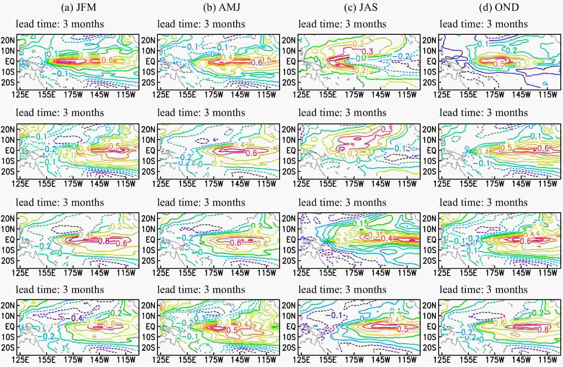 Figure10. SSTA evolution for different lead times (3, 6, 9 and 12 months), when the SSTA-OPRs are superimposed on the corresponding initial months of different seasons: (a) for March in JFM; (b) for June in AMJ; (c) for September in JAS; (d) for December in OND.
From Fig. 10, it is evident that all the SST-OPRs can evolve into El Ni?o events when superimposed on the corresponding initial seasons, and the SSTA matures in the eastern Pacific. Specifically, when adding AMJ (spring) SST-OPRs, the SSTA signal moves quickly to the central-eastern Pacific after six months and matures in the eastern Pacific via wave dynamics. When adding JFM (winter) SST-OPRs, the SSTA signal also propagates to the central-eastern Pacific and matures in the eastern Pacific. However, its variability shows a certain unstable evolution during spring, which can be caused by the spring predictability barrier (SPB) phenomenon. When adding JAS (summer) SST-OPRs, the SSTA signal fails to show growth from summer to autumn (Fig. 10c), which may be caused by the fact that the ocean tends to have a stable state during early autumn. Later, the SSTA signal is transferred to the eastern Pacific by Kelvin waves and matures in the eastern Pacific. When adding the OND (autumn) SST-OPRs, Kelvin waves are induced quickly when the ocean state is disturbed at the start time; three months later, SSTA signals propagate into the central and eastern Pacific via Kelvin waves and mature in the eastern Pacific.
In summary, four seasonal SST-OPRs can lead to the occurrence of an El Ni?o event. Although the SST-OPRs show obvious seasonal dependence, their evolution can be explained by Bjerknes-like positive feedback and thermocline feedback; that is, the wind anomaly, SSTA and thermocline anomaly over the equatorial Pacific may establish a Bjerknes-like positive feedback and thermocline feedback, which will make the evolution of the OPRs sensitive to the initial months.
First, the CNOPs for different initial months of the chosen basic years are obtained using the GD method, and the magnitudes and spatial structures of those CNOPs are investigated. The objective function values of CNOPs for different initial months exhibit particular uncertainties and are sensitive to the seasons. The largest objective function values can always be reached when the initial months are in the JFM season, whose corresponding prediction end time is at the end of the year, which can be explained by the fact that the ENSO events tend to peak at this time. The smallest values are reached when the initial months are in the JAS season, whose prediction end time is in the AMJ season (spring season). It can be implied that the objective function values of CNOPs for different initial months exhibit particular uncertainty and are sensitive to the seasons, which is associated with the SPB phenomenon. By investigating the spatial structures of those CNOPs, a positive SSTA signal is seen largely in the western-central equatorial Pacific Ocean. However, there are obvious differences in the patterns between different seasonal SST-OPRs along the equatorial western-central Pacific, showing seasonal dependence to some extent.
Then, the CNOPs are superimposed on the corresponding initial months to obtain the temporal evolution of the Ni?o3.4 index and to examine whether those CNOPs can represent the SST-OPRs of the ENSO events. The results show that basic non-El Ni?o events can eventually evolve into El Ni?o events when the CNOPs are superimposed on the basic state of the corresponding initial months; that is, the three-month running mean of the Ni?o3.4 index is above 0.5ЁуC for more than three months, which is consistent with the definition of an El Ni?o event.
Finally, the temporal evolutions of the seasonal SST-OPRs are examined to investigate the evolution of the SST-OPRs in the ICM. By superimposing the seasonal SST-OPRs on the corresponding seasons, all the SST-OPRs can evolve into El Ni?o events and the SSTA matures in the eastern Pacific. Thus, the OPRs for ENSO events in the ICM can be identified and depicted using the GD method.
In addition, the OPRs for El Ni?o show certain season dependency and positive anomalies in IOCAS ICM, while Hu and Duan (2016) found that there are two types (positive and negative) of composite patterns associated with the precursory disturbances for El Ni?o in CESM: one possesses a wide range of positive SSTAs over the equatorial Pacific, while the other consists of an SSTA component with negative anomalies in the central-eastern equatorial Pacific. It can be seen that the specific SSTA OPR patterns in the two models are not the same. But, both studies show that the peak values of Ni?o index appear at the end of the year. Therefore, it can be inferred that the OPRs for ENSO are dependent on the numerical model. It would be interesting to study the OPRs of ENSO in other kinds of models.
Note that only the initial error in the initial SST is considered in this paper. Because the SST can be affected by many other factors, such as sea level, subsurface entrainment temperature, etc., it is therefore necessary to study the OPRs for those related physical factors regardless of whether initial errors are present. In addition, not only initial-condition errors but also model-parameter errors can cause uncertainty in ENSO prediction. Therefore, it is worth studying the influence of model-parameter errors on ENSO prediction and whether these errors, as with initial-condition errors, also show certain seasonal dependence. In addition, the influence of the combination of model-parameter and initial-condition errors on ENSO prediction is another aspect worthy of study.
Acknowledgments. This work is supported by the Fundamental Research Funds for the Central Universities (Grant No. 22120190207), the Strategic Priority Research Program of the Chinese Academy of Sciences (Grant No. XDA19060102), the National Key Research and Development Program of China (Grant No. 2017YFC1404102(2017YFC1404100)), the National Programme on Global Change and Air?Sea Interaction (Grant No. GASI-IPOVAI-06), National Natural Science Foundation of China (Grant Nos. 41690122(41690120), 41490644(41490640), 41421005), and the Taishan Scholarship. Thanks to the Institute of Oceanology, Chinese Academy of Sciences, for providing technical support for IOCAS ICM. The authors also acknowledge the National Supercomputer Center in Tianjin for providing the computer resources. No conflicts of interest exist in relation to this manuscript.
