Control Research for a Small Fixed-Wing UAV During Ground Taxiing

Jiuzhou Gao^1,2, Hongguang Jia¹

(1.Changchun Institute of Optics, Fine Mechanics and Physics,Chinese Academy of Sciences, Changchun 130033, China;2.University of Chinese Academy of Sciences, Beijing 100039, China)



Abstract:

Ground taxiing is the key process of take-off and landing for a tricycle-undercarriage unmanned aerial vehicle (UAV). Nonlinear model of a sample UAV is established based on stiffness and damping model of landing gears and tires taken into account. Then lateral nonlinear model is linearized and state space equations are deduced by using nose wheel and ruder as inputs and lateral states as outputs. Adaptive internal model control (AIMC) is proposed and applied to lateral control based on decoupled and linearized dynamic model during ground taxiing process. Different control strategies are analyzed and compared by simulations, and then a combined control strategy of nose wheel steering with holding and rudder control is given. Hardware in loop simulations (HILS) proves the validity of the controller designed.

Key words:  ground taxiing  landing gears and tires model  AIMC  control strategy  HILS

DOI：10.11916/j.issn.1005-9113.15249

Clc Number:V19

Fund:


Jiuzhou Gao, Hongguang Jia. Control Research for a Small Fixed-Wing UAV During Ground Taxiing[J]. Journal of Harbin Institute of Technology, 2017, 24(2): 51-57. DOI: 10.11916/j.issn.1005-9113.15249.
Fund Sponsored by the Knowledge Innovation Project of Chinese Academy of Sciences (Grant No.YYJ-1122) Corresponding author Jiuzhou Gao, Email: gaojiuzhou@126.com Article history Received: 2015-09-01



Contents            Abstract            Full text            Figures/Tables            PDF


Control Research for a Small Fixed-Wing UAV During Ground Taxiing
Jiuzhou Gao^1,2, Hongguang Jia¹    
1. Changchun Institute of Optics, Fine Mechanics and Physics, Chinese Academy of Sciences, Changchun 130033, China;
2. University of Chinese Academy of Sciences, Beijing 100039, China

Received: 2015-09-01
Fund: Sponsored by the Knowledge Innovation Project of Chinese Academy of Sciences (Grant No.YYJ-1122)
Corresponding author: Jiuzhou Gao, Email: gaojiuzhou@126.com


Abstract: Ground taxiing is the key process of take-off and landing for a tricycle-undercarriage unmanned aerial vehicle (UAV). Nonlinear model of a sample UAV is established based on stiffness and damping model of landing gears and tires taken into account. Then lateral nonlinear model is linearized and state space equations are deduced by using nose wheel and ruder as inputs and lateral states as outputs. Adaptive internal model control (AIMC) is proposed and applied to lateral control based on decoupled and linearized dynamic model during ground taxiing process. Different control strategies are analyzed and compared by simulations, and then a combined control strategy of nose wheel steering with holding and rudder control is given. Hardware in loop simulations (HILS) proves the validity of the controller designed.
Key words: ground taxiing    landing gears and tires model    AIMC    control strategy    HILS    
1 IntroductionA tricycle-undercarriage UAV will suffer sideslip angle and lateral deviation in the conditions of winds, asymmetric configuration and rough runway, especially moment from propeller piston engineer^[1-3].Refs.[4-5] provided a kind of modeling method through landing gears and tires, but they did not consider the influence of torque from propeller, decentration from thrust and ground angle. Ref.[6] proposed neural network theory to rectify the deviation and Ref.[7] adopted neural network control to rectify the lateral deviation, but the membership function was hardly selected. Refs.[8-10] designed mixed H₂/H_∞ state feedback controllers based on genetic algorithm, which was too complex to apply in the engineering. Fuzzy control was studied by Refs.[11-13], but fuzzy rules were hardly acquired.Ref.[14] presented lateral and longitudinal control law based on gain scheduling, but it was just suitable for low speed taxiing.Refs.[15-16] proposed LQG/LTR theory which enhanced system robustness to apply on taxiing and landing control. A new approach of adaptive internal model control (AIMC) is proposed in this paper, which depends on model estimation and filter parameter adjustment^[17-20].

The sample plane is a small fixed-wing UAV, and V-tail structure is adopted and propeller piston engine is used as thrust device. Some characteristics are given in Table 1.

表 1
Table 1 Characteristics of sample UAV Parameter Value Description

c_A(m) 0.543 4 Mean aerodynamic chord

b(m) 6.051 Wing span

S_w(m²) 3.11 Wing area

m(kg) 200 Mass

V_c(km/h) 120-200 Cruise speed

H_c(m) 4 000 Cruise altitude

T_e(h) 6 Endurance time



Table 1 Characteristics of sample UAV



2 Dynamic ModelingContrast to flight in the air, ground taxiing is affected by ground characteristics except gravity, thrust, aerodynamic force and their moment. Force and moment from ground acting on the UAV are discussed in this paper. Ground characteristics include supporting force, frictional force and their moment.

2.1 Supporting ForceThere are two methods to obtain supporting force:one depends on mechanical properties, which needs amount of the compression of landing gears and tires and their compression rate; the other is to create mathematical equations based on force characteristic, and supporting force is deduced. The mathematical equations can not be always established during landing phase, especially the process of touchdown the ground instantly.The first method is adopted in this paper. Landing gears and tires can be seen as linear discrete system, the stiffness and damping are constant.

Supporting force in the earth-surface inertial reference frame is formulated as follows:

$\mathit{\boldsymbol{P}} = {\mathit{\boldsymbol{P}}_n} + {\mathit{\boldsymbol{P}}_{ml}} + {\mathit{\boldsymbol{P}}_{mr}} = \left[ {\begin{array}{*{20}{c}}0\\0\\{ - {P_n} - {P_{ml}} - {P_{mr}}}\end{array}} \right]$

where P_n denotes the pressure from nose wheel to ground; P_ml denotes the pressure from left main wheel to ground; P_mr denotes the pressure from right main wheel to ground.

The pressures of different landing gears and tiresare presented as:

$\left\{ \begin{array}{l}{P_n} = {K_n}\Delta {z_n} + {C_n}\Delta {{\dot z}_n}\\{P_{ml}} = {K_m}\Delta {z_{mr}} + {C_m}\Delta {{\dot z}_{mr}}\\{P_{mr}} = {K_m}\Delta {z_{ml}} + {C_m}\Delta {{\dot z}_{ml}}\end{array} \right.$

where K_n and C_n denote the stiffness and damping of nose landing gears and tire; Δz_n and $ \Delta {\dot z_n}$ denote the compression amount and compression rate of nose landing gears and tire; K_m and C_m denote the stiffness and damping of main landing gears and tire; Δz_mr and $\Delta {\dot z_{mr}} $ denote the compression amount and compression rate of right landing gears and tire; Δz_ml and $ \Delta {\dot z_{ml}}$ denote the compression amount and compression rate of left landing gears and tire.

The moments caused by supporting forces in body coordinate frame are expressed as:

${\mathit{\boldsymbol{M}}_p} = {\mathit{\boldsymbol{M}}_{np}} + {\mathit{\boldsymbol{M}}_{mlp}} + {\mathit{\boldsymbol{M}}_{mrp}}$

The moments caused by supporting forces of different landing gears and tires are presented as:

$\left\{ \begin{array}{l}{\mathit{\boldsymbol{M}}_{np}} = {\mathit{\boldsymbol{L}}_n} \times \left( {\mathit{\boldsymbol{DC}}{\mathit{\boldsymbol{M}}_{be}}{\mathit{\boldsymbol{P}}_n}} \right)\\{\mathit{\boldsymbol{M}}_{mlp}} = {\mathit{\boldsymbol{L}}_{ml}} \times \left( {\mathit{\boldsymbol{DC}}{\mathit{\boldsymbol{M}}_{be}}{\mathit{\boldsymbol{P}}_{ml}}} \right)\\{\mathit{\boldsymbol{M}}_{mrp}} = {\mathit{\boldsymbol{L}}_{mr}} \times \left( {\mathit{\boldsymbol{DC}}{\mathit{\boldsymbol{M}}_{be}}{\mathit{\boldsymbol{P}}_{mr}}} \right)\end{array} \right.$

where L_n, L_mland L_mr denote the centroid positions of nose wheel, left main wheel and right main wheel in the body coordinate frame respectively; DCM_be denotes the transform matrix from earth-surface inertial reference frame to body coordinate frame, and

$\mathit{\boldsymbol{DC}}{\mathit{\boldsymbol{M}}_{be}} =\\ \left[ {\begin{array}{*{20}{c}}{\cos \bar \theta \cos \phi } & {\cos \bar \theta \sin \phi } & { - \sin \bar \theta }\\{\sin \phi \sin \bar \theta \cos \psi - \cos \phi \sin \psi } & {\sin \phi \sin \bar \theta \sin \psi + \cos \phi \cos \psi } & {\sin \phi \cos \bar \theta }\\{\cos \phi \sin \bar \theta \cos \psi + \sin \phi \sin \psi } & {\cos \phi \sin \bar \theta \sin \psi - \sin \phi \cos \psi } & {\cos \phi \cos \bar \theta }\end{array}} \right]$

2.2 FrictionFriction consists of lateral friction and rolling friction. Lateral friction can be seen as a lateral sliding friction that preventing the wheels fromskidding. When the UAV makes a turn, the tires will produce lateral force that is perpendicular to rotation. There is an angle between velocity of the wheel and axis of the wheel (as shown in Fig. 1), and to define the angle as cornering angle and anticlockwise from axis of the wheel to velocity of the wheel is positive. Their relationship is a kind of nonlinear transcendental function from the elastic tire experiments. When the cornering angle is small enough (≤5°), linear relationship is held to exist as:

$\left\{ \begin{array}{l}{F_n} = {K_{\beta n}}{\beta _n}\\{F_{ml}} = {K_\beta }{\beta _{ml}}\\{F_{mr}} = {K_\beta }{\beta _{mr}}\end{array} \right.$

Figure 1
Figure 1 Ground taxiing friction



where β_n, β_ml, β_mr denote the cornering angle of nose, left and right main wheel respectively; K_βn and K_β denote the cornering stiffness of nose and main wheel.

Fig. 1 shows the friction analysis of the UAV during ground taxiing. According to Fig. 1, the cornering angle can be deduced as:

$\left\{ \begin{array}{l}{\beta _{ml}} = \arctan \left( {\frac{{r \cdot {a_m} - v}}{{u + r \cdot {b_w}/2}}} \right)\\{\beta _{mr}} = \arctan \left( {\frac{{r \cdot {a_m} - v}}{{u - r \cdot {b_w}/2}}} \right)\\{\theta _n} = \arctan \left( {\frac{{v + r \cdot {a_n}}}{u}} \right)\\{\beta _n} = {\theta _l} - {\theta _n}\end{array} \right.$

where θ_l is input angle to control nose wheel steering and anticlockwise from axis of the wheel to axis of the frame is positive; θ_n is the angle between velocity of the nose wheel and axis of the wheel and anticlockwise from axis of the wheel to velocity of the wheel is positive.

The rolling friction can be obtained as:

$\left\{ \begin{array}{l}{Q_n} = \mu {P_n}\\{Q_{ml}} = \mu {P_{ml}}\\{Q_{mr}} = \mu {P_{mr}}\end{array} \right.$

where μ is the rolling friction coefficient between tires and ground.

The friction in body coordinate frame can be summarized as:

$\begin{array}{l}\mathit{\boldsymbol{f}} = {\mathit{\boldsymbol{f}}_n} + {\mathit{\boldsymbol{f}}_{mr}} + {\mathit{\boldsymbol{f}}_{ml}} = \\\;\;\;\;\;\mathit{\boldsymbol{DC}}{\mathit{\boldsymbol{M}}_{b{w_n}}}\left[ {\begin{array}{*{20}{c}}{ - {Q_n}}\\{{F_n}}\\0\end{array}} \right] + \mathit{\boldsymbol{DC}}{\mathit{\boldsymbol{M}}_{b{w_{mr}}}}\left[ {\begin{array}{*{20}{c}}{ - {Q_{mr}}}\\{{F_{mr}}}\\0\end{array}} \right] + \\\;\;\;\;\;\mathit{\boldsymbol{DC}}{\mathit{\boldsymbol{M}}_{b{w_{ml}}}}\left[ {\begin{array}{*{20}{c}}{ - {Q_{ml}}}\\{{F_{ml}}}\\0\end{array}} \right]\end{array}$

where DCM_bwn,^DCM_bwmland DCM_bwmr denote transform matrix from nose wheel, left main wheel and right main wheel to body coordinate frame, and

$\begin{array}{*{20}{c}}{\mathit{\boldsymbol{DC}}{\mathit{\boldsymbol{M}}_{b{w_n}}} = \\\left[ {\begin{array}{*{20}{c}}{\cos \bar \theta \cos {\theta _l}} & {\cos \bar \theta \sin {\theta _l}} & { - \sin \bar \theta }\\{\sin \phi \sin \bar \theta \cos {\theta _l} - \cos \phi \sin {\theta _l}} & {\sin \phi \sin \bar \theta \sin {\theta _l} + \cos \phi \cos {\theta _l}} & {\sin \phi \cos \bar \theta }\\{\cos \phi \sin \bar \theta \cos {\theta _l} + \sin \phi \sin {\theta _l}} & {\cos \phi \sin \bar \theta \sin {\theta _l} - \sin \phi \cos {\theta _l}} & {\cos \phi \cos \bar \theta }\end{array}} \right]}\\{\mathit{\boldsymbol{DC}}{\mathit{\boldsymbol{M}}_{b{w_{ml}}}} = \mathit{\boldsymbol{DC}}{\mathit{\boldsymbol{M}}_{b{w_{ml}}}} = \left[ {\begin{array}{*{20}{c}}{\cos \bar \theta } & 0 & { - \sin \bar \theta }\\{\sin \phi \sin \bar \theta } & {\cos \phi } & {\sin \phi \cos \bar \theta }\\{\cos \phi \sin \bar \theta } & { - \sin \phi } & {\cos \phi \cos \bar \theta }\end{array}} \right]}\end{array}$

The moments caused by frictions in the body coordinate frame can be expressed by:

${\mathit{\boldsymbol{M}}_f} = {\mathit{\boldsymbol{M}}_{fn}} + {\mathit{\boldsymbol{M}}_{fml}} + {\mathit{\boldsymbol{M}}_{fmr}}$

The moments of different landing gears and tiresare presented as:

$\left\{ \begin{array}{l}{\mathit{\boldsymbol{M}}_{fn}} = {\mathit{\boldsymbol{L}}_n} \times {\mathit{\boldsymbol{f}}_n}\\{\mathit{\boldsymbol{M}}_{fml}} = {\mathit{\boldsymbol{L}}_{ml}} \times {\mathit{\boldsymbol{f}}_{ml}}\\{\mathit{\boldsymbol{M}}_{fmr}} = {\mathit{\boldsymbol{L}}_{mr}} \times {\mathit{\boldsymbol{f}}_{mr}}\end{array} \right.$

Finally, the forces and moments during ground taxiing in the body coordinate frame can be summarized as:

$\left\{ \begin{array}{l}\mathit{\boldsymbol{F}} = {\mathit{\boldsymbol{M}}_{bg}}\mathit{\boldsymbol{G}} + {\mathit{\boldsymbol{M}}_{ba}}\mathit{\boldsymbol{R}} + \mathit{\boldsymbol{T}} + {\mathit{\boldsymbol{M}}_{bg}}\mathit{\boldsymbol{P}} + \mathit{\boldsymbol{f}}\\\mathit{\boldsymbol{M}} = {\mathit{\boldsymbol{M}}_\mathit{\boldsymbol{R}}} + {\mathit{\boldsymbol{M}}_\mathit{\boldsymbol{T}}} + {\mathit{\boldsymbol{M}}_\mathit{\boldsymbol{P}}} + {\mathit{\boldsymbol{M}}_\mathit{\boldsymbol{f}}}\end{array} \right.$

where G is gravity; R is aerodynamic force; T is thrust from piston propeller engine; M_R is aerodynamic moment; M_T is thrust moment; M_bg is transform matrix from ground to body coordinate frame; M_ba is transform matrix from aerodynamic to body coordinate frame; M_bs is transform matrix from stability to body coordinate frame.

2.3 Linearized ModelingSmall perturbation theory is used to make the nonlinear mathematical model linearized. Making the following assumption that criterion movement is along the runway centerline, states of longitudinal movement are invariable to keep a constant.

The decoupled lateral nonlinear mathematical model is calculated by:

$\left\{ \begin{array}{l}\dot \beta = - r\cos \bar \theta + \frac{Y}{{mV}} + \frac{{{f_y}}}{{mV}}\cos \beta - \frac{{T\cos \left( {{\alpha _T} + \bar \theta } \right)}}{{mV}}\sin \beta - \\\;\;\;\;\;\;\frac{{{f_x}}}{{mV}}\sin \beta \\\dot r = {c_9}\left[ {\bar N + {T_{or}}\sin {\alpha _T} - \left( {{F_{ml}} + {F_{mr}}} \right){a_m}\cos \bar \theta + } \right.\\\;\;\;\;\;\left( {{F_n}\cos {\theta _l} - {Q_n}\sin {\theta _l}} \right){a_n}\cos \bar \theta + \\\;\;\;\;\;\left. {\left( {\mu - \tan \bar \theta } \right)\left( {{T_{or}}\cos {\alpha _T} + \bar L + {M_{fx}}} \right)} \right]\end{array} \right.$

The lateral linearized model are expressed in the state space equations as:

$\mathit{\boldsymbol{\dot x}} = \mathit{\boldsymbol{Ax}} + \mathit{\boldsymbol{Bu}}$

where state vector x=[β r]^T, input vector u=[θ_l δ_r]^T, input matrix:

$\mathit{\boldsymbol{B}} = \left[ {\begin{array}{*{20}{c}}{ - \frac{{{f_y}^{\left( {{\theta _l}} \right)}}}{{mV}}} & {\frac{{{Y^{\left( {{\delta _r}} \right)}}}}{{mV}}}\\{{c_9}\left[ {\left( {F_n^{\left( {{\theta _l}} \right)} - \mu {P_n}} \right){a_n}\cos \bar \theta + \left( {\mu - \tan \bar \theta } \right)M_{fx}^{\left( {{\theta _l}} \right)}} \right]} & {{c_9}{{\bar N}^{\left( {{\delta _r}} \right)}}}\end{array}} \right]$

State matrix:

$\mathit{\boldsymbol{A}} = \left[ {\begin{array}{*{20}{c}}{\frac{{{Y^{\left( \beta \right)}}}}{{mV}} + \frac{{{f_y}^{\left( \beta \right)}}}{{mV}} - \frac{{T\cos \left( {{\alpha _T} + \bar \theta } \right)}}{{mV}}{\rm{ - }}\frac{{{f_x}}}{{mV}}} & { - \cos \bar \theta + \frac{{{f_y}^{\left( r \right)}}}{{mV}} + \frac{{{Y^{\left( r \right)}}}}{{mV}}}\\{{c_9}\left[ {{{\bar N}^{\left( \beta \right)}} - {M^{\left( \beta \right)}} + \left( {\mu - \tan \bar \theta } \right)M_{fx}^{\left( \beta \right)}} \right]} & {\;{c_9}\left[ {{{\bar N}^{\left( r \right)}} - {M^{\left( r \right)}} + \left( {\mu - \tan \bar \theta } \right)M_{fx}^{\left( r \right)}} \right]}\end{array}} \right]$

Where ${M^{\left( \beta \right)}} = \left( {F_{ml}^{^{\left( \beta \right)}} + F_{mr}^{^{\left( \beta \right)}}} \right){a_m}\cos \bar \theta + F_n^{^{\left( \beta \right)}}{a_n}\cos \bar \theta ,{M^{\left( r \right)}} = \left( {F_{ml}^{^{\left( r \right)}} + F_{mr}^{^{\left( r \right)}}} \right){a_m}\cos \bar \theta + F_n^{^{\left( r \right)}}{a_n}\cos \bar \theta $.

3 Controller DesignInternal model control usually consists of controlled process, process model and controller with filter, which is a model-based design approach, the structure of conventional IMC is shown in Fig. 2.

Figure 2
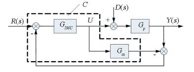Figure 2 Conventional internal model control



The design procedure of IMC usually has two steps, decomposing the process model as Eq.(1) and controller design with filter as Eqs.(2) and (3).

${G_m}\left( s \right) = {G_{m + }}\left( s \right) \cdot {G_{m - }}\left( s \right)$ (1)

${G_{IMC}} = G_{m - }^{ - 1}\left( s \right)F\left( s \right)$ (2)

$F\left( s \right) = \frac{1}{{{{\left( {\varepsilon s + 1} \right)}^\gamma }}}$ (3)

where G_m+(s) and G_m-(s) are the portions of the model not inverted and inverted respectively; G_m+(s) contains all the dead time and right half plane zeros of G_p(s), while G_m-(s) is stable and has the minimum phase; ε denotes time constant and γ denotes relative order of the filter.

There is only one degree of freedom for conventional IMC structure, filter parameter is only a trade-off between dynamic performance and system robustness.To achieve a good dynamic performance and strong system robustness, parameter adjustment and model estimation are proposed. The AIMC structure is shown in Fig. 3.

Figure 3
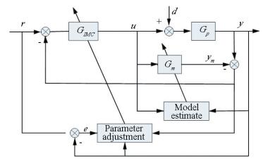Figure 3 Adjustment internal model control



Filter parameter should be a small value when initial selected, which will be better for the dynamic response, when the mode error becomes bigger and threatens the system stability, the filter parameter should be adaptive amplification to ensure system stability. Adaptive law of filter parameter is:

$\varepsilon = {\varepsilon _0}\left( {1 + \int_{{t_r}}^{{t_s}} {\left| e \right|\left| {\frac{{y - {y_m}}}{{{y_m}}}} \right|{\rm{d}}t} } \right)$

where ε₀ denotes initial filter parameter; e denotes system error; y denotes system output; y_m denotes output of process model; t_r denotes the first time of achieving system setting point and t_s denotes system regulation time.

Least squares method is used for process model estimation, considering the following system model:

$\begin{array}{l}\mathit{\boldsymbol{y}}\left( n \right) = - {a_1}\mathit{\boldsymbol{y}}\left( {n - 1} \right) - {a_2}\mathit{\boldsymbol{y}}\left( {n - 2} \right) - \cdots + \\\;\;\;\;\;\;{{\rm{b}}_0}\mathit{\boldsymbol{u}}\left( {n - k} \right) + {b_1}\mathit{\boldsymbol{u}}\left( {n - k - 1} \right) + \\\;\;\;\;\;\; \cdots + \mathit{\boldsymbol{\omega }}\left( n \right) = {\mathit{\pmb{\phi}} ^{\rm{T}}}\mathit{\boldsymbol{\theta }} + \mathit{\boldsymbol{\omega }}\left( n \right)\end{array}$

where φ denotes observation vector of input and output; θ denotes unknown parameter vector; ω denotes white noise.

$\begin{array}{*{20}{c}}{{\mathit{\pmb{\phi}} ^{\rm{T}}} = \left[ { - y\left( {n - 1} \right),y\left( {n - 2} \right), \cdots ,y\left( {n - k} \right),u\left( {n - m} \right),u\left( {n - m - 1} \right), \cdots ,u\left( {n - m - k} \right)} \right]}\\{\mathit{\boldsymbol{\theta = }}\left[ {{a_1},{a_2}, \cdots ,{a_k},{b_0},{b_1}, \cdots ,{b_k}} \right]}\end{array}$

Recursive algorithm of the unknown parameter vector of least squares method is present as:

$\left\{ \begin{array}{l}\mathit{\boldsymbol{\hat \theta }}\left( {n + 1} \right) = \mathit{\boldsymbol{\hat \theta }}\left( n \right) + K\left( {n + 1} \right)\left[ {y\left( {n + 1} \right) - } \right.\\\;\;\;\;\;\;\;\;\;\;\;\;\;\;\;\left. {{\mathit{\pmb{\phi}} ^{\rm{T}}}\left( {n + 1} \right)\mathit{\boldsymbol{\hat \theta }}\left( n \right)} \right]\\\mathit{\boldsymbol{K}}\left( {n + 1} \right) = \frac{{P\left( n \right)\mathit{\pmb{\phi}} \left( {n + 1} \right)}}{{1 + {\mathit{\pmb{\phi}} ^{\rm{T}}}\left( {n + 1} \right)P\left( n \right)\mathit{\pmb{\phi}} \left( {n + 1} \right)}}\\\mathit{\boldsymbol{P}}\left( {n + 1} \right) = \left[ {1 - \mathit{\boldsymbol{K}}\left( {n + 1} \right){\mathit{\pmb{\phi}} ^{\rm{T}}}\left( {n + 1} \right)} \right]\mathit{\boldsymbol{P}}\left( n \right)\end{array} \right.$

4 Control StrategyElevator produces some pressure-head moment to ensure the efficiency of nose wheel steering during three-wheel taxiing. When the airspeed achieves 120 km/h, elevator gives out -10°, and the rise-head moment would make three-wheel taxiing transfer to two-wheel taxiing, and the pith angle should be limited to prevent the tail of frame touching the ground.

Taking the takeoff process as example, yaw angle and lateral deviation do not adopt control firstly, and states are analyzed throughout simulation. Initial airspeed is 0.1 m/s, and initial position is (0, 0, 0), and ground angle is 0.8°. The simulation is stopped as soon as all the wheels leaving the ground.

Fig. 4 shows longitudinal state histories including pith angle, altitude, airspeed and elevator. Pith angle is always keeping ground angle until taking off instantaneously and the setting of initial altitude would cause little vibration of pith angle at the beginning. As airspeed and lift increase, the amount of compression of land gears and tires would decrease, altitude rises with taxiing. As soon as air speed achieves 120 km/s, the elevator instruct transfers from positive to negative, altitude falls down little instantaneously as the increase of the amount of compression of main wheels, then lift increases quickly and takes off.

Figure 4
Figure 4 Longitudinal state histories



Fig. 5 shows lateral state histories including yaw angle, lateral deviation, nose wheel steering angle and output of rudder. The frame will taxi to the right direction as the reason of symmetric configuration and the moment from propeller piston engineer. The yaw angle reaches 7°and lateral deviation attains 30 m when leaving ground.

Figure 5
Figure 5 Lateral state histories without control



To eliminate the errors of yaw angle and lateral deviation, nose wheel steering control is adopted. As it is dangerous to change the steering angle at high airspeed, Fig. 6(a) illustrates the state histories using the nose wheel steering at low airspeed, control switch point is 20 m/s of airspeed, yaw angle and lateral deviation is very little during lateral control phase, when the airspeed achieves 20 m/s, nose wheel angle returns to zero, the remaining taxiing does not adopt lateral control, the final yaw angle is 4°and lateral deviation 8.5 m when leaving ground. Contrast to Fig. 6(a), Fig. 6(b) shows state histories using nose wheel steering with holding nose angle after node airspeed, and the result is better than the former, and the final yaw angle is 0.5°and lateral deviation 0.9 m when leaving ground.

Figure 6
Figure 6 Lateral state histories with nose wheel control



As nose steering control is not suitable for high airspeed, rudder control is utilized for lateral control after 20 m/s of airspeed. Fig. 7(a)gives out the state histories of combined control but without holding nose angle. When the airspeed achieves switch point of airspeed, nose wheel angle returns to zero and rudder control becomes effective, yaw angle and lateral deviation come to zero as the use of rudder. Contrast to Fig. 7(a), Fig. 7(b) shows the state histories of combined control with holding nose angle. When the airspeed achieves 20 m/s, nose wheel angle holding current angle and rudder control becomes effective at the same time, the yaw angle and lateral deviation vary smaller and the output of rudder is less than the former.

Figure 7
Figure 7 Lateral state histories with combined control



To verify the robustness of control system, initial offset and crosswind are added in simulations respectively. Fig. 8 illustrates state histories with initial yaw angle 10°and lateral deviation 2 m, to eliminate the errors of yaw angle and lateral deviation, the nose wheel steering angle attains saturation, the errors come to zero with taxiing.

Figure 8
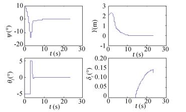Figure 8 Lateral state with initial offset



Crosswind of 8 m/s is brought in the simulation, the results are shown in Fig. 9. The action point of crosswind is V tail mainly, hence negative yaw angle comes to emergence, but positive lateral deviation generates because of positive flight-path angle. To eliminate the error of yaw angle, the nose wheel steering gives positive steering angle and rudder negative instruct, and lateral deviation is small enough at the same time.

Figure 9
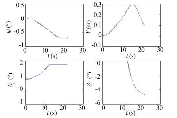Figure 9 Lateral state with initial offset



5 Hardware in Loop SimulationTo prove the validity of controller designed, hardware in loop simulations is made. Hardware in loop platform usually consists of ground station, model simulator, airborne computer, three-axis simulation platform, load simulator, servos and various sensors.

The results are shown in Figs. 10 and 11. Compared with Fig. 4 and Fig. 7(b) respectively, the longitudinal states are the same basically. There is some difference between lateral states. Negative initial lateral deviation exists in HILS, and the nose wheel steering angle is positive at the beginning, after switch point airspeed, the rudder gives out positive instruct to eliminate the yaw angle and lateral deviation.

Figure 10
Figure 10 Longitudinal state of HILS



Figure 11
Figure 11 Lateral state of HILS



6 ConclusionsThis paper elaborates a systematic process to modeling, controller and strategy design, and simulations during ground taxiing phase. Ground characteristics are taken into account. Parameters of landing gears and tires are key point for modeling. Different control strategies are analyzed by AIMC throughout simulations, combined strategy of nose wheel steering with holding and rudder control is better than others. Hardware in loop simulations proves the validity of the system.


References
[1] Dension N A. Design of Automated Carrier Landing of an Unmanned Combat Aerial Vehicle Using Dynamic Inversion. Islamabad: Air University, 2007. (0)

[2] Volkan K. Design of Automatic Carrier Landing of an Unmanned Aerial Vehicle Using Dynamic Inversion. Ankara: Middle East Technical University, 2007. (0)

[3] Singh S, Padhi R. Automatic path planning and control design for autonomous landing of UAVs using dynamic inversion. Proceedings of 2009 American Control Conference. Piscataway: IEEE, 2009. 2409-2414. DOI: 10.1109/ACC.2009.5160444. (0)

[4]Chen Chen, Zhou Zhou. Process and mathematic model study of a UAV during taxiing and takeoff.Science Technology and Engineering, 2007, 7(13): 3198-3201.(0)

[5]Duan Songyun, Zhu Jihong, Sun Zengqi. Model study of a UAV during landing with three wheels in ground motion.Journal of System Simulation, 2004, 16(6): 1296-1299.DOI:10.16182/j.cnki.joss.2004.06.050(0)

[6]Akesson B M, Toivonen H T. A neural network model predictive controller.Journal of Control, 2006, 16(9): 937-946.DOI:10.1016/j.jprocont.2006.06.01(0)

[7]Wang Yong, Wang Yingxun. Lateral deviation correction control for UAV taxiing.ACTA Aeronautica ET Astronautica Sinica, 2008, 29(Sup.): 142-149.(0)

[8]Pan Wei, Wang Xueyong, Jing Yuanwei. Mixed H₂/H_∞state feedback controllers based on genetic algorithm.Control and Decision, 2005, 20(2): 132-136.(0)

[9]Santoso F, Liu M. H₂/H_∞robust autopilot synthesis for longitudinal flight of a special unmanned aerial vehicle:A comparative study.Control Theory & Applications, 2008(7): 583-594.DOI:10.1049/iet-cta:20070415(0)

[10] Wang Ren. Flying-wing UAV landing control and simulation based on mixed H₂/H_∞. Proceedings of the International Conference on Mechatronics and Automation. Piscataway: IEEE, 2007. 1523-1528. DOI: 10.1109/ICMA.2007.4303775. (0)

[11]Yuan Chaohui, Wang Yi, Yang Fang. Application of new fuzzy control in air planes'integrated ground directional control.Journal of System simulation, 2011, 28(2): 76-79.(0)

[12] Li B, Jiao Z, Wang S. Research on modeling and simulation of aircraft taxiing rectification. Proceedings of the IEEE Conference on Robotics, Automation and Mechatronics. Piscataway: IEEE, 2006. 1-5. DOI: 10.1109/RAMECH.2006.252621. (0)

[13] Zhang Fan, Wang Yong. Automatic landing of unmanned aerial vehicle using fuzzy control. Proceeding of the IEEE International Conference on Information and Automation. Piscataway: IEEE, 2013. 472-477. (0)

[14]Duan Zhen, Gao Jiuzhou. Linearized modeling and gain scheduling control for UAV taxiing.Optics and Precision Engineering, 2014, 22(6): 1507-1516.DOI:10.3788/OPE.(0)

[15] Garcia L, Lopez M J, Jamshidi M. LQG/LTR and fault detection filter design for a flight control system application. Proceedings of the World Automation Congress. Piscataway: IEEE, 2004. No. 04EX832C. (0)

[16] Gargouri L, Zaafouri A. LQG / LTR control of a direct current motor. Proceedings of the IEEE International Conference on Systems, Man and Cybernetics, 2002. Piscataway: IEEE, 2002. DOI: 10.1109/ICSMC.2002.1176354. (0)

[17]Rupp D, Guzzella L. Iterative tuning of internal model controllers application to air/fuel ratio control.IEEE Transactions on Control Systems Technology, 2010, 18(1): 177-184.DOI:10.1109/TCST.2008.2010458(0)

[18]Alcantara S, Pedret C, Vilanova R, et al. Generalized internal model control for balancing input/output disturbance response.Industry Engineering Chemistry Research, 2011, 50(19): 70-80.DOI:10.1021/ie200717z(0)

[19] Astrom K J, Wittenmark B. Adaptive Control. Boston, MA: Addison-Wesley Longman Publishing, Inc. , 2008. (0)

[20]Ferrari S, Stengel R F. Online adaptive critic flight control.AIAA Journal of Guidance, Control and Dynamics, 2004, 27(5): 777-786.DOI:10.2514/1.12597(0)