Jing Zhang, Dehua Wen^,, Yuxi LiSchool of Physics and Optoelectronics, South China University of Technology, Guangzhou 510641, China

Received:2021-03-5Revised:2021-07-21Accepted:2021-07-21Online:2021-09-17


Abstract
Due to improvements in the sensitivity of gravitational wave (GW) detectors, the detection of GWs originating from the fundamental quasi-normal mode (f-mode) of neutron stars has become possible. The future detection of GWs originating from the f-mode of neutron stars will provide a potential way to improve our understanding of the nature of nuclear matter inside neutron stars. In this work, we investigate the constraint imposed by the f-mode oscillation of neutron stars on the symmetry energy of nuclear matter using Bayesian analysis and parametric EOS. It is shown that if the frequency of the f-mode of a neutron star of known mass is observed precisely, the symmetry energy at twice the saturation density (E_sym(2ρ₀)) of nuclear matter can be constrained within a relatively narrow range. For example, when all the following parameters are within the given intervals: 220 ≤ K₀ ≤ 260 MeV, 28 ≤ E_sym(ρ₀) ≤ 36 MeV, 30 ≤ L ≤ 90 MeV, −800 ≤ J₀ ≤ 400 MeV, − 400 ≤ K_sym ≤ 100 MeV, −200 ≤ J_sym ≤ 800 MeV, E_sym(2ρ₀) will be constrained to within ${48.8}_{-5.5}^{+6.6}$ MeV if the f-mode frequency of a canonical neutron star (1.4 M_⊙) is observed to be 1.720 kHz with a 1% relative error. Furthermore, if only f-mode frequency detection is available, i.e. there is no stellar mass measurement, a precisely detected f-mode frequency can also impose an accurate constraint on the symmetry energy. For example, given the same parameter space and the same assumed observed f-mode frequency mentioned above, and assuming that the stellar mass is in the range of 1.2–2.0 M_⊙, E_sym(2ρ₀) will be constrained to within ${49.5}_{-6.8}^{+8.1}\,\mathrm{MeV}$. In addition, it is shown that a higher slope of 69 ≤ L ≤ 143 MeV will give a higher posterior distribution of E_sym(2ρ₀), ${53.8}_{-6.4}^{+7.0}\,\mathrm{MeV}$.
Keywords： f-mode;Bayesian analysis;nuclear symmetry energy;neutron star


PDF (1259KB)MetadataMetricsRelated articlesExportEndNote|Ris|BibtexFavorite
Cite this article
Jing Zhang, Dehua Wen, Yuxi Li. Constraint on nuclear symmetry energy imposed by f-mode oscillation of neutron stars. Communications in Theoretical Physics, 2021, 73(11): 115302- doi:10.1088/1572-9494/ac1669

1. Introduction

Neutron stars may oscillate nonradially and emit gravitational waves (GWs) when they are disturbed by external or internal events [1, 2]. These GWs are generally expected to provide useful information about the stellar structure and the equation of state (EOS) of the dense nuclear matter of neutron stars [3–5]. It is hoped that the features of GWs from the quasi-normal modes will be verified by advanced GW detectors such as the Einstein Telescope in the near future [6, 7]. Among the multitudinous oscillation modes, the f-mode has received particular attention [3, 5, 8, 9]. Normally, researchers start from the EOS and the differential equation of f-mode oscillation to calculate and analyze its characteristic parameters, such as its frequency and damping time [10–13]. During the last twenty years or so, a number of works have focused on the inverse problem, that is, to extract information about the EOS of neutron star matter from the future measurement of gravitational waves related to f-mode oscillations [3–5, 10, 14–17]. The basic approach of these works is to find the universal relations between the f-mode parameters and the global properties of neutron stars, then constrain the global properties (in particular, the mass and the radius) of neutron stars through the universal relations and the assumed observed parameters of the oscillation modes, and finally, according to the constrained global properties, impose a qualitative constraint on the EOS of the dense nuclear matter [3–5, 10, 14–16]. In this work, we will use a totally different approach to solve the inverse problem, namely, Bayesian analysis. This method makes it convenient to combine the various latest astronomical observations and the most recent developments in nuclear physics to obtain a relatively strict and reliable constraint on the neutron star properties and the equation of state [18].

The fundamental mode (f-mode) is regarded as one of the most important modes, as its lower frequency (1 ∼ 3 kHz) makes it relatively easier to observe than the other modes using existing observation apparatus [19]. For example, for a neutron star located 10kpc from us, it is estimated that the f-mode energy required for detection with a signal-to-noise ratio of ten by the advanced LIGO detector is 8.7 × 10⁻⁷ M_⊙, which is far smaller than those of the p-mode and the w-mode [5]. Recently, W C G Ho et al found that the GW bursts from f-mode oscillations, thought to be excited by known pulsar glitches, are observable by current GW detectors (Advanced LIGO/Virgo/Kagra) [20]. They further pointed out that a significant number of events will be observed by the next-generation detectors. For this reason, we only focus here on the f-modes when we investigate the constraint on the symmetry energy of nuclear matter imposed by the oscillation modes.

As we know, it is the EOS (basically seen as the density–pressure relation) that determines the macroscopic properties of neutron stars, such as the stellar mass, radius, moment of inertia, tidal deformability, and so on. However, until today, the EOS of extremely dense nuclear matter has remained the largest mystery in nuclear physics, as it is hard to reproduce extremely dense nuclear matter, similar to the core of a neutron star, in a terrestrial laboratory. One of the main sources of uncertainty in the EOS is the lack of knowledge of the density dependence of the nuclear symmetry energy at super-high densities, E_sym(ρ) [21, 22].

Fortunately, astronomical observations related to pulsars provide an effective way to understand the EOS of nuclear matter [23–29]. The detection of gravitational waves from a binary neutron star merger (GW170817) has sparked a great deal of research into constraining the EOS of extremely dense nuclear matter, as the tidal effect (characterized by tidal deformability) strongly depends on the EOS [30–34]. Considering that the f-mode is likely to be observed in the near future, it would thus be very interesting to investigate the constraint on the features of nuclear matter imposed by the f-mode oscillations of neutron stars.

In fact, we have done some exploratory work in this area [17], in which the symmetry energy at twice the saturation density (E_sym(2ρ₀)) was directly constrained by an assumed observed frequency with a fixed stellar mass and each of the parametric EOSs produced had equal weights; in other words, the previous constraint on E_sym(2ρ₀) was an a priori constraint. In addition, there are only three varying parameters (J₀, K_sym, and J_sym) in the EOS model. According to [17], it has been shown that E_sym(2ρ₀) could be prior constrained within 54.5 ± 6.5 MeV if the f-mode frequency of a canonical neutron star were to take a value of 1.64 kHz with a 1% relative error. In order to obtain a more rational constraint, we reinvestigate this problem in this work by employing Bayesian inference in a larger parameter space, that is, six parameters (E_sym(ρ₀), L, K₀, J₀, K_sym, and J_sym) of the EOS model are used as varying parameters. Moreover, as it is not easy to precisely detect both the parameters of the f-mode oscillation and the stellar mass, the constraints on the symmetry energy based on the f-mode frequency observation alone are also investigated.

This paper is organized as follows. In section 2, the isospin-dependent parametric EOS of dense neutron-rich nucleonic matter and the basic formulas for f-mode oscillation in neutron stars are briefly reviewed. In section 3, the constraints imposed on the symmetry energy by Bayesian analysis using the assumed observed frequency of the f-mode are presented and discussed. A summary of the main points is given at the end.

2. Brief introduction to parametric EOS and the basic formulas of the f-mode

2.1. The isospin-dependent parametric EOS

Here, we give a brief review of the isospin-dependent parametric EOS, in which dense nuclear matter is supposed to be composed of neutrons, protons, electrons, and muons at β-equilibrium under the charge-neutrality condition [23, 26]. The energy density of dense nuclear matter with an isospin asymmetry of δ = (ρ_n − ρ_p)/ρ at a density ρ can be expressed as(2.1)$\begin{eqnarray}\epsilon (\rho ,\delta )=\rho \left[E(\rho ,\delta )+{M}_{{\rm{N}}}\right]+{\epsilon }_{{\rm{l}}}(\rho ,\delta ),\end{eqnarray}$where M_N (= 939 MeV) is the average nucleon mass, ε_l(ρ, δ) is the lepton energy density, and E(ρ, δ) is the nucleon-specific energy. Given the energy density, the pressure of dense nuclear matter can be calculated through(2.2)$\begin{eqnarray}p(\rho ,\delta )={\rho }^{2}\displaystyle \frac{{\rm{d}}(\epsilon (\rho ,\delta )/\rho )}{{\rm{d}}\rho }.\end{eqnarray}$For the energy density of neutron-rich nuclear matter, the specific energy of the nucleon E(ρ, δ) is the most important but also the most difficult factor to determine. It can be closely approximated by the empirical parabolic law, as follows [21, 35]:(2.3)$\begin{eqnarray}E(\rho ,\delta )={E}_{0}(\rho )+{E}_{\mathrm{sym}}(\rho )\cdot {\delta }^{2}+O({\delta }^{4}),\end{eqnarray}$where E₀(ρ) is the specific energy of symmetric nuclear matter and E_sym(ρ) is the symmetry energy of asymmetric nuclear matter. They can be parameterized by the following equations [23]:(2.4)$\begin{eqnarray}\begin{array}{rcl}{E}_{0}(\rho ) & = & {E}_{0}({\rho }_{0})+\displaystyle \frac{{K}_{0}}{2}{\left(\displaystyle \frac{\rho -{\rho }_{0}}{3{\rho }_{0}}\right)}^{2}\\ & & +\displaystyle \frac{{J}_{0}}{6}{\left(\displaystyle \frac{\rho -{\rho }_{0}}{3{\rho }_{0}}\right)}^{3},\end{array}\end{eqnarray}$and(2.5)$\begin{eqnarray}\begin{array}{rcl}{E}_{\mathrm{sym}}(\rho ) & = & {E}_{\mathrm{sym}}({\rho }_{0})+L\left(\displaystyle \frac{\rho -{\rho }_{0}}{3{\rho }_{0}}\right)\\ & & +\displaystyle \frac{{K}_{\mathrm{sym}}}{2}{\left(\displaystyle \frac{\rho -{\rho }_{0}}{3{\rho }_{0}}\right)}^{2}+\displaystyle \frac{{J}_{\mathrm{sym}}}{6}{\left(\displaystyle \frac{\rho -{\rho }_{0}}{3{\rho }_{0}}\right)}^{3}.\end{array}\end{eqnarray}$where ρ₀ is the nuclear saturation density (ρ₀ = 0.16 fm⁻³) and E₀(ρ₀) = −15.9 MeV [21]. Based on nuclear laboratory experiments and theoretical predictions [36–41], the currently known ranges of the asymptotic values of the EOS parameters near the saturation density can be summarized as follows: 220 ≤ K₀ ≤ 260 MeV, 28 ≤ E_sym(ρ₀) ≤ 36 MeV, 30 ≤ L ≤ 90 MeV, −800 ≤ J₀ ≤ 400 MeV, −400 ≤ K_sym ≤ 100 MeV, and −200 ≤ J_sym ≤ 800 MeV. For more details of the parametric EOS model, please refer to [23]. It is worth noting that when the density approaches ρ₀, equations (2.4) and (2.5) become Taylor expansions. However, in the description of super-high-density nuclear matter, the coefficients become free parameters to be determined by the observations of neutron stars and high-energy heavy-ion reaction experiments [23].

In this work, the core of the neutron star is described by the parametric EOS. The inner and outer crusts of the neutron star are connected by the Negele-Vautherin (NV) EOS [42] and the Baym-Pethick-Sutherland (BPS) EOS [43], respectively. The crust–core transition point is estimated by a thermodynamical approach. The thermodynamical stability conditions require positive compressibility $-{\left(\tfrac{\partial P}{\partial \nu }\right)}_{q}\gt 0$ and stability of the charge fluctuations ${\left(\tfrac{\partial \mu }{\partial q}\right)}_{P}\gt 0$ [44, 45]. By employing beta-equilibrium baryon number conservation and charge conservation, the crust–core transition density in parametrized EOS can be obtained by the following equation [22, 23]:(2.6)$\begin{eqnarray}\begin{array}{l}{\rho }^{2}\displaystyle \frac{{{\rm{d}}}^{2}{E}_{0}}{{\rm{d}}{\rho }^{2}}+2\rho \displaystyle \frac{{\rm{d}}{E}_{0}}{{\rm{d}}\rho }+{\delta }^{2}\left[{\rho }^{2}\displaystyle \frac{{{\rm{d}}}^{2}{E}_{\mathrm{sym}}}{{\rm{d}}{\rho }^{2}}+2\rho \displaystyle \frac{{\rm{d}}{E}_{\mathrm{sym}}}{{\rm{d}}\rho }\right.\\ \,-\ \left.2{E}_{\mathrm{sym}}^{-1}{\left(\rho \displaystyle \frac{{\rm{d}}{E}_{\mathrm{sym}}}{{\rm{d}}\rho }\right)}^{2}\right]=0.\end{array}\end{eqnarray}$For details of the method used to estimate the crust–core transition point, please refer to [23].

By varying the parameters E_sym(ρ₀), L, K₀, J₀, K_sym, and J_sym within their allowed ranges, we can generate a sufficiently large number of EOSs to perform the Bayesian analysis. Compared with the multisegment polytropic EOS, the parametric EOS model provides a more convenient way to extract the symmetry energy of the asymmetric nuclear matter from the astronomical observations. It is worth pointing out that before we perform the Bayesian analysis, the EOSs are first screened against broadly accepted constraints, such as the causality condition [46–50], agreement with massive neutron star observations [51], and support of the observational constraints on tidal deformability obtained from the detection of GW170817 [23, 52].

2.2. Basic formulas for f-mode oscillation in neutron stars

Based on the notation of Lindblom and Detweiler, the perturbed metric of a non-radial oscillating neutron star in the Regge-Wheeler gauge can be written as follows [11, 12]:(2.7)$\begin{eqnarray}\begin{array}{rcl}{{\rm{d}}{s}}^{2} & = & -{{\rm{e}}}^{\nu }\left(1+{r}^{l}{H}_{0}(r){{\rm{Y}}}_{m}^{l}{{\rm{e}}}^{{\rm{i}}\omega t}\right){\rm{d}}{t}^{2}\\ & & -2{\rm{i}}\omega {r}^{l+1}{H}_{1}(r){{\rm{Y}}}_{m}^{l}{{\rm{e}}}^{{\rm{i}}\omega t}{\rm{d}}t{\rm{d}}r\\ & & +{{\rm{e}}}^{\lambda }\left(1-{r}^{l}{H}_{0}(r){{\rm{Y}}}_{m}^{l}{{\rm{e}}}^{{\rm{i}}\omega t}\right){\rm{d}}{r}^{2}\\ & & +{r}^{2}\left(1-{r}^{l}K(r){{\rm{Y}}}_{m}^{l}{{\rm{e}}}^{{\rm{i}}\omega t}\right)\left({\rm{d}}{\theta }^{2}+{\sin }^{2}\theta {\rm{d}}{\phi }^{2}\right),\end{array}\end{eqnarray}$where ν and λ are the unperturbed metric functions, only the functions r, H₀(r), H₁(r), and K(r) describe the perturbations of spacetime, and Y_m^l is the spherical harmonic function.

The components of the Lagrangian displacement of the fluid elements can be expressed as follows [11, 12]:(2.8)$\begin{eqnarray}{\xi }^{r}={r}^{l-1}{{\rm{e}}}^{-\lambda /2}W(r){{\rm{Y}}}_{m}^{l}{{\rm{e}}}^{{\rm{i}}\omega t},\end{eqnarray}$(2.9)$\begin{eqnarray}{\xi }^{\theta }=-{r}^{l-2}V(r){\partial }_{\theta }{{\rm{Y}}}_{m}^{l}{{\rm{e}}}^{{\rm{i}}\omega t},\end{eqnarray}$(2.10)$\begin{eqnarray}{\xi }^{\phi }=-{r}^{l}{\left(r\sin \theta \right)}^{-2}V(r){\partial }_{\phi }{{\rm{Y}}}_{m}^{l}{{\rm{e}}}^{{\rm{i}}\omega t},\end{eqnarray}$where W(r) and V(r) are the only functions of r.

As a consequence of Einstein's equation, the perturbation functions above are not all independent. For example, the perturbed metric function H₀(r) can be represented by the other two perturbed functions, H₁(r) and K (r), as given in [11, 12]:(2.11)$\begin{eqnarray}\begin{array}{rcl}{H}_{0}(r) & = & {\left[3M+\displaystyle \frac{1}{2}(l+2)(l-1)r+4\pi {r}^{3}p\right]}^{-1}\\ & & \times \left\{8\pi {r}^{3}{{\rm{e}}}^{-\nu /2}-\left[\displaystyle \frac{1}{2}l(l+1)\left(M+4\pi {r}^{3}p\right)\right.\right.\\ & & \left.-{\omega }^{2}{r}^{3}{{\rm{e}}}^{-(\lambda +\nu )}\right]{H}_{1}(r)\\ & & +\left[\displaystyle \frac{1}{2}(l+2)(l-1)r-{\omega }^{2}{r}^{3}{{\rm{e}}}^{-\nu }\right.\\ & & \left.\left.-\left(M+4\pi {r}^{3}p\right)\left(3M-r+4\pi {r}^{3}p\right)K(r)\right]\right\}.\end{array}\end{eqnarray}$It is convenient to define the following function X(r), rather than using the function V(r) to solve the perturbed Einstein equations [12]:(2.12)$\begin{eqnarray}\begin{array}{rcl}X(r) & = & {\omega }^{2}(\rho +p){{\rm{e}}}^{-\nu /2}V(r)\\ & & -{p}^{\,^{\prime} }{r}^{-1}{{\rm{e}}}^{(\nu -\lambda )/2}W(r)+\displaystyle \frac{1}{2}(\rho +p){{\rm{e}}}^{\nu /2}{H}_{0}(r).\end{array}\end{eqnarray}$

Based on the linearized Einstein equations(2.13)$\begin{eqnarray}\delta {G}_{\mu \nu }=8\pi \delta {T}_{\mu \nu },\end{eqnarray}$and the conservation equation(2.14)$\begin{eqnarray}\delta {{T}^{\mu \nu }}_{;\,\mu }=0,\end{eqnarray}$where ‘;' represents the covariant derivative, a set of equations for H₁(r), K(r), W(r), and X(r) can be obtained, as follows [11, 12, 53]:(2.15)$\begin{eqnarray}\begin{array}{rcl}{H}_{1}^{{\prime} }(r) & = & -{r}^{-1}\left[l+1+2{{Mr}}^{-1}{{\rm{e}}}^{\lambda }+4\pi {r}^{2}{{\rm{e}}}^{\lambda }(p-\rho )\right]{H}_{1}(r)\\ & & +{r}^{-1}{{\rm{e}}}^{\lambda }\left[{H}_{0}(r)+K(r)-16\pi \left(p+\rho \right)V(r)\right],\end{array}\end{eqnarray}$(2.16)$\begin{eqnarray}\begin{array}{rcl}{K}^{{\prime} }(r) & = & {r}^{-1}{H}_{0}(r)+\displaystyle \frac{1}{2}l(l+1){r}^{-1}{H}_{1}(r)\\ & & -\left[(l+1){r}^{-1}-\displaystyle \frac{1}{2}{\nu }^{{\prime} }\right]K(r)\\ & & -8\pi \left(p+\rho \right){{\rm{e}}}^{\lambda /2}{r}^{-1}W(r),\end{array}\end{eqnarray}$(2.17)$\begin{eqnarray}\begin{array}{rcl}{W}^{{\prime} }(r) & = & -(l+1){r}^{-1}W(r)+r{{\rm{e}}}^{\lambda /2}\left[{\gamma }^{-1}{p}^{-1}{{\rm{e}}}^{-\nu /2}X(r)\right.\\ & & \left.-(l+1){r}^{-2}V(r)+\displaystyle \frac{1}{2}{H}_{0}(r)+K(r)\right],\end{array}\end{eqnarray}$(2.18)$\begin{eqnarray}\begin{array}{rcl}{X}^{{\prime} }(r) & = & -{{lr}}^{-1}X(r)+\left(p+\rho \right){{\rm{e}}}^{\nu /2}\left\{\displaystyle \frac{1}{2}\left({r}^{-1}-\displaystyle \frac{1}{2}{\nu }^{{\prime} }\right){H}_{0}(r)\right.\\ & & +\displaystyle \frac{1}{2}\left[r{\omega }^{2}{{\rm{e}}}^{-\nu }+\displaystyle \frac{1}{2}l(l+1){r}^{-1}\right]{H}_{1}(r)\\ & & +\displaystyle \frac{1}{2}\left(\displaystyle \frac{3}{2}{\nu }^{{\prime} }-{r}^{-1}\right)K(r)-\displaystyle \frac{1}{2}l(l+1){\nu }^{{\prime} }{r}^{-2}V(r)\\ & & -{r}^{-1}\left[4\pi \left(p+\rho \right){{\rm{e}}}^{\lambda /2}+{\omega }^{2}{{\rm{e}}}^{\lambda /2-\nu }\right.\\ & & \left.\left.-\displaystyle \frac{1}{2}{r}^{2}{\left({r}^{-2}{{\rm{e}}}^{-\lambda /2}{\nu }^{{\prime} }\right)}^{{\prime} }\right]W(r)\right\},\end{array}\end{eqnarray}$where ‘′’ represents the first derivative of the radius, such as ${X}^{{\prime} }=\tfrac{{\rm{d}}X}{{\rm{d}}r}$, and the quantity $\gamma =\tfrac{\rho +p}{p}\tfrac{{\rm{d}}p}{{\rm{d}}\rho }$ is the adiabatic index.

The boundary conditions for H₁(r) and X(r) can be obtained using the regularity requirement at the center; the pressure, which approaches zero at the surface, provides another boundary condition for X(r), as it is directly related to the Lagrangian perturbation of pressure. These three conditions are sufficient to solve the perturbed equations inside the star. The eigenfrequencies of the purely outgoing modes can be obtained by matching the interior solution to the Zerilli function of the exterior solution [8]. For the detailed numerical method, please refer to [8, 11, 12].

3. Constraints on the symmetry energy of dense nuclear matter imposed by the parameters of f-mode oscillation under Bayesian analysis

As we saw in the last section, due to the complexity of the f-mode formulas, it is hard to reversely solve the EOS based only on the formulas and the assumed observed parameters of the f-mode. Fortunately, Bayesian analysis provides an effective method with which to solve this reverse problem. Furthermore, Bayesian analysis can combine various observational data to constrain the EOS.

The posterior probability of Bayesian analysis is given by(3.1)$\begin{eqnarray}P({ \mathcal M }| D)=\displaystyle \frac{P\left(D| { \mathcal M }\right)P({ \mathcal M })}{\int P(D| { \mathcal M })P({ \mathcal M }){\rm{d}}{ \mathcal M }},\end{eqnarray}$where $P({ \mathcal M }| D)$ is the posterior probability of model ${ \mathcal M }$ for the given datum D, and $P(D| { \mathcal M })$ is the likelihood function. In this work, the model ${ \mathcal M }$ will represent the set of parameters (J₀, K_sym, J_sym) of the parametric EOS, and the datum D is the assumed observed frequency of the f-mode. We define the likelihood function as follows:(3.2)$\begin{eqnarray}P(D| { \mathcal M })=\displaystyle \frac{1}{\sqrt{2\pi }{\sigma }_{{\rm{ob}}}}\exp \left[-\displaystyle \frac{{\left({\nu }_{{\rm{th}}}-{\nu }_{{\rm{ob}}}\right)}^{2}}{2{\sigma }_{{\rm{ob}}}^{2}}\right],\end{eqnarray}$where ν_th is the theoretical calculated frequency of f-mode, ν_ob is the assumed observed frequency and σ_ob is its error. Combining equations (3.1) and (3.2), we can calculate the probability distribution function (PDF) of the EOS parameters and further analyze the symmetry energy of the dense nuclear matter through the Bayesian inference approach. In this work, we use the Markov chain Monte Carlo procedure introduced by Zhang et al [54].

We uniformly sample the parameters in each interval: 220 ≤ K₀ ≤ 260 MeV, 28 ≤ E_sym(ρ₀) ≤ 36 MeV, 30 ≤ L ≤ 90 MeV, −800 ≤ J₀ ≤ 400 MeV, −400 ≤ K_sym ≤ 100 MeV, and −200 ≤ J_sym ≤ 800 MeV to generate the corresponding EOSs for each set of parameters. We then screen the EOSs using the causality, the maximum observed mass, and the tidal deformability parameters. If the EOS satisfies these conditions, we further calculate the f-mode frequency. The calculated frequency is used as the theoretical frequency v_th in the likelihood function equation (3.2). Since the f-mode gravitational wave signal has not been detected so far, the assumed observed frequency v_ob in equation (3.2) is just a hypothetical observed value. In this work, the most probable frequency in the prior distribution (as shown in figure 1) is used as the assumed observed frequency v_ob.

Figure 1.

New window|Download| PPT slide
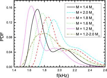
Figure 1.The prior distribution of f-mode frequencies of a neutron stars with known stellar masses and unknown stellar masses (assumed to be within 1.2–2.0 M_⊙) under the simplified (set E_sym(ρ₀) = 31.7 MeV, L = 58.7 MeV, K₀ = 240 MeV) parametric EOSs, which are already screened by the causality condition, the masses of observed massive neutron stars, and the tidal deformability of GW170817.


In order to select a relatively rational f-mode frequency as the assumed observed value, we use the posterior distribution of the isospin-dependent EOS parameters [52] to regenerate about two hundred thousand EOSs. Using these EOSs, we calculated the distribution of the f-mode frequencies of neutron stars with fixed stellar masses (1.2, 1.4, 1.6, 1.8, and 2.0 M_⊙) and with variable stellar masses (assumed to be within 1.2–2.0 M_⊙, which cover most of the observed masses of neutron stars [55]). We take this distribution as the prior distribution in this work, as shown in figure 1. It is worth noting that the EOSs used to calculate the distribution are simplified by fixing three parameters as constants: K₀ = 240 MeV [37], E_sym (ρ₀) = 31.7 MeV [40], and L = 58.7 MeV [23, 38]. It is shown that a more massive star corresponds to a higher most probable frequency. For a canonical neutron star (M = 1.4 M_⊙), the most probable frequency is about 1.720 kHz. For an unknown-mass neutron star, the most probable f-mode frequency is about 1.830 kHz if we assume its mass is in the range of 1.2–2.0 M_⊙.

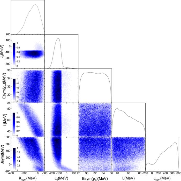
If the f-mode frequency of a canonical neutron star is observed in the near future, it will provide a valuable way to reversely constrain the EOS of the dense nuclear matter. We adopt three assumed observed f-mode frequencies of canonical neutron stars, including the most probable frequency, 1.720 kHz, to reversely constrain the parameters E_sym(ρ₀), L, K₀, J₀, K_sym and J_sym, and further constrain the symmetry energy by employing Bayesian analysis. Figure 2 shows the posterior distributions of the EOS parameters (K_sym, J₀, E_sym(ρ₀), L, J_sym) and their correlations. It can be seen that the parameters J₀ and K_sym are relatively well constrained, while J_sym prefers larger values and L prefers smaller values. Our calculations show that the parameters K₀ (not shown in this figure) and E_sym(ρ₀) are not affected by the observed f-mode frequencies of canonical neutron stars. These constraints are consistent with results constrained by the radii of canonical neutron stars [26]. As for the correlations, it is obvious that there are stronger anti-correlations between K_sym and L and between K_sym and J_sym. We can understand this point using the explanation given in [26], which is that two adjacent parameters can compensate for each other to rebuild the same results under the same conditions.

Figure 2.

New window|Download| PPT slide
Figure 2.The posterior distributions and correlations of K_sym, J₀, E_sym(ρ₀), L, and J_sym constrained by an assumed observed frequency of 1.720 kHz with a one percent relative error for a canonical neutron star (M = 1.4 M_⊙).


As we know, in many references, researchers have adopted the symmetry energy at twice the saturation density (E_sym(2ρ₀)) as a representative point to show the constraints imposed on the symmetric energy of high-density nuclear matter by astronomical observations [17, 24, 26, 27]. For example, through simultaneously analyzing the data from terrestrial nuclear experiments and astrophysical observations (including electromagnetic and gravitational measurements), Zhou et al [24] concluded that E_sym(2ρ₀) should be in the range of $[{39.4}_{-6.4}^{+7.5}$, ${54.5}_{-3.2}^{+3.1}]$ MeV. According to three sets of observational radii data and three sets of imaginary radii data for a canonical neutron star, Xie and Li [26] constrained the symmetry energy to twice the saturation density at E_sym(2ρ₀) = ${39.2}_{-8.2}^{+12.1}$ MeV at a 68% credible level using the Bayesian analysis method and a parametric EOS model. By comprehensively combining the observational results for the radius, maximum mass, and tidal deformability of neutron stars, Zhang and Li [27] gave the constraint as E_sym(2ρ₀) = 46.9 ± 10.1 MeV. By supposing that the frequency of a canonical neutron star's f-mode takes a value of f = ${1.640}_{-0.016}^{+0.016}$ kHz and that each of the parametric EOSs has equal weight, Wen et al [17] obtained a prior constraint on E_sym(2ρ₀) in the range of ${54.5}_{-6.5}^{+6.5}\,\mathrm{MeV}$, where only the parameters J₀, K_sym, and J_sym were mutable in the parametric EOS. It is worth pointing out that the last constraint on the symmetry energy is derived from hypothetical data, rather than being based on real observations.

Based on the posterior distributions obtained for E_sym(ρ₀), L, K_sym, and J_sym using the parametric EOS, we can further constrain the symmetry energy of high-density nuclear matter according to equation (2.5). For the convenience of comparison with other references [17, 24, 26, 27], here, we also mainly probe the symmetry energy at twice the saturation density (E_sym(2ρ₀)). The posterior distribution of E_sym(2ρ₀) is presented in figure 3. It is shown that at a 90% posterior credibility level and taking a 1% relative error for the assumed observed f-mode frequency of a canonical neutron star, E_sym(2ρ₀) is constrained to lie within ${55.3}_{-5.5}^{+6.0}$ MeV for 1.640 kHz, ${48.8}_{-5.5}^{+6.6}$ MeV for 1.720 kHz, and ${43.8}_{+6.0}^{-6.0}$ MeV for 1.800 kHz, respectively.

Figure 3.

New window|Download| PPT slide
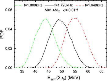
Figure 3.The posterior distribution of E_sym(2ρ₀) constrained by assumed observed frequencies of 1.640 kHz, 1.720 kHz, and 1.800 kHz with a one percent relative error for a canonical neutron star (M = 1.4 M_⊙).


In [56–58], it is shown that the crust–core transition point has significant impact on the crust thickness and the moment of inertia of the crust, and has a weak influence on the stellar radius; a unified EOS model was employed in their investigations. As the EOS of the inner crust has a notable influence on the stellar radius [59], and the frequency of the f-mode is sensitive to the radius of the neutron star [4], it is interesting to probe the effect of the inner-crust EOS on the constraint on E_sym(2ρ₀) obtained from the assumed observed f-mode frequency. To probe the impact of the crust's EOS, we replace the EOS of the inner crust by a polytropic form p = a + bρ^λ [60], where λ = 4/3, 6/3, and 8/3, corresponding to different softnesses. As the influence of the outer crust's EOS on the stellar radius is very weak, we still connected the outer crust using the BPS EOS. Using the constructed EOS for the inner crust, we calculated the effect of the EOS of the inner crust. Our calculations show that the difference in the inner-crust EOS model has a slight influence on the constraint on E_sym(2ρ₀).

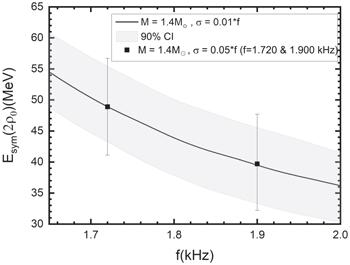
As shown in figure 3, it is easy to see that for the canonical neutron star, a smaller f-mode frequency gives a relatively higher E_sym(2ρ₀). In order to express more clearly and quantitatively how E_sym(2ρ₀) changes along with the f-mode frequency, figure 4 contains a plot showing the most probable value of E_sym(2ρ₀) as a function of the f-mode frequency (at a 1% relative error) of a canonical neutron star. It is shown that for a canonical neutron star, a lower f-mode frequency such as f ∼ 1.60 kHz, needs E_sym(2ρ₀) to be around 57 MeV, while a higher frequency such as f ∼ 2.0 kHz will give a relatively lower value, ∼36 MeV for E_sym(2ρ₀). We can understand this result using the universal relation [61]. As shown in Figure 3 in [61], there is a linear universal relation between the scaled frequency Mω of the f-mode and the compactness M/R of a neutron star. For neutron stars with a fixed stellar mass (e.g. 1.4 M_⊙), a higher scaled frequency corresponds to greater compactness, that is, to a smaller stellar radius. In general, for a neutron star with a fixed stellar mass, the smaller the radius, the softer the corresponding symmetry energy of the EOS. To investigate the effect of measurement accuracy on the constraints, we add the posterior distributions of two points (f = 1.720 & 1.900 kHz) at a 5% relative error in figure 4. It is shown that with a decrease in the observation accuracy, the center value of E_sym(2ρ₀) stays about the same, but the error range increases.

Figure 4.

New window|Download| PPT slide
Figure 4.The most probable E_sym(2ρ₀) as a function of the f-mode frequency (with a 1% relative error) of a canonical neutron star, where the gray area denotes the uncertainty band at a 90% credibility level. For comparison, the posterior distributions of two points (f = 1.720 & 1.900 kHz) with a 5% relative error are also presented.


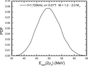
As we know, it is not easy to accurately measure both the stellar mass and the f-mode frequency of a neutron star using the known GW detectors. If we only detect the f-mode frequency accurately, can we also impose a meaningful constraint on the symmetry energy? The answer is yes! In order to select an appropriate value for the assumed observation value, we first calculate the most probable value of the f-mode frequency under the prior distribution by assuming that the stellar mass is limited to the range 1.2–2.0 M_⊙. We also choose 1.720 kHz as the assumed observed frequency of the f-mode for a mass-unknown neutron star. The posterior constraints on E_sym(2ρ₀) based only on the assumed frequency of the f-mode are plotted in figure 5, in which the assumed observed frequency is 1.720 kHz with one percent of relative error, and the stellar mass is limited to the range 1.2 − 2.0 M_⊙. The results show that even though we cannot detect the stellar mass, the observed f-mode frequency can also impose a relatively good constraint on the symmetry energy. For example, if we observe a 1.720 kHz f-mode frequency for a neutron star, we can constrain E_sym(2ρ₀) to ${49.5}_{-6.8}^{+8.1}\,\mathrm{MeV}$.

Figure 5.

New window|Download| PPT slide
Figure 5.The posterior distribution of E_sym(2ρ₀) constrained by an assumed observed frequency of 1.720 kHz with a one percent relative error, where the stellar masses are limited to the range 1.2–2.0 M_⊙.


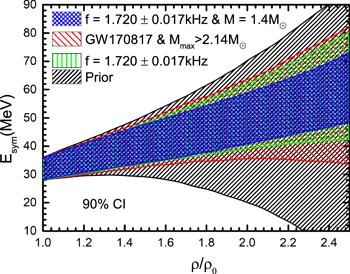
In order to more intuitively show the degrees of constraint on the symmetry energy under different conditions, we plot four different constraints in figure 6, in which the black area represents the prior constraint without any screening conditions imposed on the parametric EOSs, the red area represents the prior constraint in which the EOSs are screened using the three abovementioned conditions, the green area represents the 90% credibility-level posterior constraint based only on an assumed observed frequency of 1.720 kHz with 1% of relative error, and the blue area represents a posterior constraint similar to (c) but for a canonical neutron star with a 1.720 kHz f-mode frequency. Clearly, if we can precisely detect both the f-mode frequency and the stellar mass for the same neutron star, we can impose a stricter constraint on the symmetry energy of nuclear matter.

Figure 6.

New window|Download| PPT slide
Figure 6.Different constraints on the symmetry energy E_sym(ρ). (a) The black area represents the prior constraint for which no screening conditions are imposed on the EOSs. (b) The red area represents the prior constraint for which the EOSs are screened by the abovementioned three conditions. (c) The green area represents the posterior constraint (with a 90% credibility interval) for an assumed observed frequency if 1.720 kHz (with 1% of relative error). (d) The blue area represents a posterior constraint similar to (c) but for a canonical neutron star with a 1.720 kHz f-mode frequency.


Recently, through exploiting the strong correlation between the neutron skin thickness of ²⁰⁸Pb and the density dependence of the symmetry energy L, the PREX Collaboration (where PREX is short for the ²⁰⁸Pb Radius Experiment) derived a relatively higher slope L, namely, 69 ≤ L ≤ 143 MeV [62, 63]. How does the higher slope L affect the symmetry energy at 2ρ₀? In figure 7, we plot the posterior distributions of the symmetry energy at 2ρ₀ for the two cases of 30 ≤ L ≤ 90 MeV and 69 ≤ L ≤ 143 MeV. As expected, compared with the ${E}_{\mathrm{sym}}(2{\rho }_{0})={48.8}_{-5.5}^{+6.6}$ MeV of 30 ≤ L ≤ 90 MeV, the higher slope (69 ≤ L ≤ 143 MeV) gives a higher symmetry energy (${E}_{\mathrm{sym}}(2{\rho }_{0})={53.8}_{-6.4}^{+7.0}$ MeV).

Figure 7.

New window|Download| PPT slide
Figure 7.The posterior distribution of the symmetry energy, E_sym(2ρ₀), for 30 ≤ L ≤ 90 MeV and 69 ≤ L ≤ 143 MeV.


Incidentally, if we want to investigate the constraint on the symmetry energy imposed by the f-mode frequency of a massive neutron star, a relatively higher assumed frequency should be selected, as hinted in figure 1. We expect that the change in the posterior distribution along with the changes of the assumed observation frequency and the observation accuracy will be similar to those of the canonical neutron star.

4. Summary

By employing Bayesian analysis, it is shown that precise measurement of the f-mode frequency and the stellar mass of a neutron star will improve our understanding of neutron-rich high-density nuclear matter. In this work, we investigate the constraints imposed on the symmetry energy of extremely dense nuclear matter by the parameter of the f-mode oscillation of a neutron star. The main results can be summed up as follows. (1) If the frequency of the f-mode of a neutron star of known mass is observed precisely, E_sym(2ρ₀) can be constrained to a relatively narrow range. For example, a canonical neutron star with a 1.720 kHz f-mode frequency with a 1% relative error constrains the E_sym(2ρ₀) to lie within the range of ${48.8}_{-5.5}^{+6.6}$ MeV when all the parameters are within their corresponding intervals (220 ≤ K₀ ≤ 260 MeV, 28 ≤ E_sym(ρ₀) ≤ 36 MeV, 30 ≤ L ≤ 90 MeV, −800 ≤ J₀ ≤ 400 MeV, −400 ≤ K_sym ≤ 100 MeV, −200 ≤ J_sym ≤ 800 MeV). (2) If only f-mode frequency detection is available, i.e. there is no stellar mass measurement, a precisely detected f-mode frequency can also impose an accurate constraint on the symmetry energy. For example, in the same parameter space and with the same assumed observed f-mode frequency mentioned above and assuming that the stellar mass is in the range of 1.2–2.0 M_⊙, E_sym(2ρ₀) will be constrained to lie within the range of ${49.5}_{-6.8}^{+8.1}$ MeV. (3) Our results further confirm that higher frequencies of the f-mode prefer a relatively lower E_sym(2ρ₀). (4) The recent measurement of a neutron skin in ²⁰⁸Pb prefers a relatively higher slope of the symmetry energy, 69 ≤ L ≤ 143 MeV. It is shown that a higher slope (69 ≤ L ≤ 143 MeV) gives a higher posterior distribution of E_sym(2ρ₀) (${53.8}_{-6.4}^{+7.0}$ MeV). In the future, if we can simultaneously measure the stellar mass, the f-mode frequency, and the damping time of a neutron star, we can obtain more precise constraints on the EOS of the neutron star matter. Moreover, if we can further obtain other observations of the global properties of neutron stars, such as the stellar radius and the moment of inertia, we can hopefully extract more useful information about the EOS of extremely dense nuclear matter by using Bayesian analysis.

Acknowledgments

We thank Mr. Houyuan Chen for helpful discussions. This work is supported by the NSFC (Grants No. 11 975 101 and No. 11 722 546), the Guangdong Natural Science Foundation (Grant No.2020A1515010820), and the talent program of South China University of Technology (Grant No. K5180470). This project has made use of NASA's Astrophysics Data System.

Reference View Option By original order
By published year
By cited within times
By Impact factor

[1]Kokkotas K D Schmidt B G 1999 Liv. Rev. Relat. 2 2
DOI:10.12942/lrr-1999-2 [Cited within: 1]

[2]Andersson N et al. 2011 Gen. Rel. Grav. 43 409
DOI:10.1007/s10714-010-1059-4 [Cited within: 1]

[3]Andersson N Kokkotas K D 1996 Phys. Rev. Lett. 77 4134
DOI:10.1103/PhysRevLett.77.4134 [Cited within: 4]

[4]Andersson N Kokkotas K D 1998 Mon. Not. R. Astron. Soc. 299 1059
DOI:10.1046/j.1365-8711.1998.01840.x [Cited within: 1]

[5]Kokkotas K D Apostolatos T A Andersson N 2001 Mon. Not. R. Astron. Soc. 320 307
DOI:10.1046/j.1365-8711.2001.03945.x [Cited within: 5]

[6]Pitkin M Reid S Rowan S Hough J 2011 Living Rev. Relativ. 14 5
DOI:10.12942/lrr-2011-5 [Cited within: 1]

[7]http://et-gw.eu/index.php/etsensitivities
[Cited within: 1]

[8]Lioutas G Stergioulas N 2018 Gen. Relativ. Gravit. 50 12
DOI:10.1007/s10714-017-2331-7 [Cited within: 3]

[9]Pratten G Schmidt P Hinderer T 2020 Nat. Commun. 11 2553
DOI:10.1038/s41467-020-15984-5 [Cited within: 1]

[10]Benhar O Ferrari V Gualtieri L 2004 Phys. Rev. D 70 124015
DOI:10.1103/PhysRevD.70.124015 [Cited within: 3]

[11]Detweiler S L Lindblom L 1985 Astrophys. J. 292 12
DOI:10.1086/163127 [Cited within: 5]

[12]Lindblom L Detweiler S L 1983 Astrophys. J. S. 53 73
DOI:10.1086/190884 [Cited within: 6]

[13]Chandrasekhar S Ferrari V 1991 Proc. R. Soc. A 434 449
[Cited within: 1]

[14]Ferrari V Miniutti G Pons J A 2003 Mon. Not. R. Astron. Soc. 342 629
DOI:10.1046/j.1365-8711.2003.06580.x [Cited within: 2]

[15]Ferrari V Gualtieri L 2008 Gen. Relativ. Gravit. 40 945
DOI:10.1007/s10714-007-0585-1

[16]Lin W K Li B A Chen L W 2014 J. Phys. G 41 075203
DOI:10.1088/0954-3899/41/7/075203 [Cited within: 1]

[17]Wen D H Li B A Chen H Y Zhang N B 2019 Phys. Rev. C 99 045806
DOI:10.1103/PhysRevC.99.045806 [Cited within: 6]

[18]Abbott B P et al. (The LIGO Scientific Collaboration and the Virgo Collaboration) 2019 Phys. Rev. Lett. 123 011102
DOI:10.1103/PhysRevLett.123.011102 [Cited within: 1]

[19]Lau H K Leung P T Lin L M 2010 Astrophys. J. 714 1234
DOI:10.1088/0004-637X/714/2/1234 [Cited within: 1]

[20]Ho W C G Jones D I Andersson N Espinoza C M 2020 Phys. Rev. D 101 103009
DOI:10.1103/PhysRevD.101.103009 [Cited within: 1]

[21]Li B A Chen L W Ko C M 2008 Phys. Rep. 464 113
DOI:10.1016/j.physrep.2008.04.005 [Cited within: 3]

[22]Lattimer J M Prakash M 2007 Phys. Rep. 442 109
DOI:10.1016/j.physrep.2007.02.003 [Cited within: 2]

[23]Zhang N B Li B A Xu J 2018 Astrophys. J. 859 90
DOI:10.3847/1538-4357/aac027 [Cited within: 9]

[24]Zhou Y Chen L W Zhang Z 2019 Phys. Rev. D 99 121301(R)
DOI:10.1103/PhysRevD.99.121301 [Cited within: 3]

[25]Zhou Y Chen L W 2019 Astrophys. J. 886 52
DOI:10.3847/1538-4357/ab4adf

[26]Xie W J Li B A 2019 Astrophys. J. 883 174
DOI:10.3847/1538-4357/ab3f37 [Cited within: 6]

[27]Zhang N B Li B A 2019 Eur. Phys. J. A 55 39
DOI:10.1140/epja/i2019-12700-0 [Cited within: 3]

[28]Zhang N B Li B A 2020 Astrophys. J. 879 99
DOI:10.3847/1538-4357/ab24cb

[29]Zhang N B Li B A 2020 Astrophys. J. 893 61
DOI:10.3847/1538-4357/ab7dbc [Cited within: 1]

[30]Paschalidis V Yagi K Alvarez-Castillo D Blaschke D B Sedrakian A 2018 Phys. Rev. D 97 084038
DOI:10.1103/PhysRevD.97.084038 [Cited within: 1]

[31]Burgio G F Drago A Pagliara G Schulze H J Wei J B 2018 Astrophys. J. 860 139
DOI:10.3847/1538-4357/aac6ee

[32]Malik T Alam N Fortin M Providencia C Agrawal B K Jha T K Kumar B Patra S K 2018 Phys. Rev. C 98 035804
DOI:10.1103/PhysRevC.98.035804

[33]Carson Z Steiner A W Yagi K 2019 Phys. Rev. D 99 043010
DOI:10.1103/PhysRevD.99.043010

[34]Abbott B P et al. (The LIGO Scientific Collaboration and the Virgo Collaboration) 2018 Phys. Rev. Lett. 121 161101
DOI:10.1103/PhysRevLett.121.161101 [Cited within: 1]

[35]Bombaci I Lombardo U 1991 Phys. Rev. C 44 1892
DOI:10.1103/PhysRevC.44.1892 [Cited within: 1]

[36]Shlomo S Kolomietz V M Colo G 2006 Eur. Phys. J. A 30 23
DOI:10.1140/epja/i2006-10100-3 [Cited within: 1]

[37]Piekarewicz J 2010 J. Phys. G 37 064038
DOI:10.1088/0954-3899/37/6/064038 [Cited within: 1]

[38]Li B A Han X 2013 Phys. Lett. B 727 276
DOI:10.1016/j.physletb.2013.10.006 [Cited within: 1]

[39]Zhang N B Cai B J Li B A Newton W G Xu J 2017 Nucl. Sci. Tech. 28 181
DOI:10.1007/s41365-017-0336-2

[40]Oertel M Hempel M Klahn T Typel S 2017 Rev. Mod. Phys. 89 015007
DOI:10.1103/RevModPhys.89.015007 [Cited within: 1]

[41]Li B A 2017 Nuclear Physics News 27 7
DOI:10.1080/10619127.2017.1388681 [Cited within: 1]

[42]Negele J W Vautherin D 1973 Nucl. Phys. A 207 298
DOI:10.1016/0375-9474(73)90349-7 [Cited within: 1]

[43]Baym G Pethick C J Sutherland P 1971 Astrophys. J. 170 299
DOI:10.1086/151216 [Cited within: 1]

[44]Kubis S 2004 Phys. Rev. C 70 065804
DOI:10.1103/PhysRevC.70.065804 [Cited within: 1]

[45]Kubis S 2007 Phys. Rev. C 76 025801
DOI:10.1103/PhysRevC.76.025801 [Cited within: 1]

[46]Keister B D Polyzou W N 1996 Phys. Rev. C 54 2023
DOI:10.1103/PhysRevC.54.2023 [Cited within: 1]

[47]Alsing J Silva H O Berti E 2018 Mon. Not. R. Astron. Soc. 478 1377
DOI:10.1093/mnras/sty1065

[48]Tews I Carlson J Gandolfi S Reddy S 2018 Astrophys. J. 860 149
DOI:10.3847/1538-4357/aac267

[49]Zhang N Wen D H Chen H Y 2019 Phys. Rev. C 99 035803
DOI:10.1103/PhysRevC.99.035803

[50]Rhoades C E Ruffini R 1974 Phys. Rev. Lett. 32 324
DOI:10.1103/PhysRevLett.32.324 [Cited within: 1]

[51]Cromartie H T et al. 2020 Nat Astron 4 72
DOI:10.1038/s41550-019-0880-2 [Cited within: 1]

[52]Li Y X Chen H Y Wen D H Zhang J 2021 Eur. Phys. J. A 57 31
DOI:10.1140/epja/s10050-021-00342-w [Cited within: 2]

[53]Thorne K S Campolattaro A 1967 Astrophys. J. 149 591
DOI:10.1086/149288 [Cited within: 1]

[54]Zhang L A et al. 2018 Comput. Chem. Eng. 110 1
DOI:10.1016/j.compchemeng.2017.11.011 [Cited within: 1]

[55]https://stellarcollapse.org/nsmasses.html
[Cited within: 1]

[56]Fortin M et al. 2016 Phys. Rev. C 94 035804
DOI:10.1103/PhysRevC.94.035804 [Cited within: 1]

[57]Carreau T Gulminelli F Margueron J 2019 Phys. Rev. C 100 055803
DOI:10.1103/PhysRevC.100.055803

[58]Piekarewicz J Fattoyev F J Horowitz C J 2014 Phys. Rev. C 90 015803
DOI:10.1103/PhysRevC.90.015803 [Cited within: 1]

[59]Huang Q Z Wen D H 2011 Commun. Theor. Phys. 55 729
DOI:10.1088/0253-6102/55/4/40 [Cited within: 1]

[60]Carriere J Horowitz C J Piekarewicz J 2003 Astrophys. J. 593 463
DOI:10.1086/376515 [Cited within: 1]

[61]Tsui L K Leung P T 2005 Mon. Not. R. Astron. Soc. 357 1029
DOI:10.1111/j.1365-2966.2005.08710.x [Cited within: 2]

[62]Adhikari D et al. (PREX Collaboration) 2021 Phys. Rev. Lett. 126 172502
DOI:10.1103/PhysRevLett.126.172502 [Cited within: 1]

[63]Reed B T et al. 2021 Phys. Rev. Lett. 126 172503
DOI:10.1103/PhysRevLett.126.172503 [Cited within: 1]