SIS Model of Rumor Spreading in Social Network with Time Delay and Nonlinear Functions
本站小编 Free考研考试/2022-01-02
Linhe Zhu,1, Xiaoyuan HuangFaculty of Science, Jiangsu University, Zhenjiang, 212013, China
First author contact:1Author to whom any correspondence should be addressed. Received:2019-07-28Revised:2019-09-5Accepted:2019-10-16Online:2019-12-30
Fund supported:
*National Natural Science Foundation of China.11571170 Natural Science Research of the Jiangsu Higher Education Institutions of China.19KJB110001 National Natural Science Foundation of China of Jiangsu Province, China.SBK20190836
Abstract With the advent of the information age of networks, the study about rumor propagation in social networks has become increasingly significant. In this paper, a rumor propagation model with nonlinear functions and time delay in social networks is proposed. First, according to the next-generation matrix method, we work out the basic reproduction number. Second, we discuss the existence of the rumor-prevailing equilibrium points. Third, we demonstrate the stabilities of equilibrium points and analyze the sufficient conditions for Hopf bifurcation. Finally, the correctness of the theory is verified and several vital conclusions are obtained by numerical simulations. Keywords:social networks;rumor spreading;delay;stability;bifurcation
PDF (946KB)MetadataMetricsRelated articlesExportEndNote|Ris|BibtexFavorite Cite this article Linhe Zhu, Xiaoyuan Huang. SIS Model of Rumor Spreading in Social Network with Time Delay and Nonlinear Functions*. Communications in Theoretical Physics, 2020, 72(1): 015002- doi:10.1088/1572-9494/ab4ef6
1. Introduction
With the rapid popularity and development of the Internet, people’s lives are greatly facilitated. The diversified network provides an important platform for people to obtain and exchange information. However, such a network inevitably also has negative effects. For example, as a social phenomenon, today’s rumors are spread through social networks, which rapidly increases their propagation speed, propagation scope and influence. When harmful rumors spread on social networks, they often have a negative impact on people’s lives and even lead to social panic and instability. Therefore, increasing importance has been attached to explore the propagation rules of rumors to find effective strategies to suppress them on social networks.
Rumor spread began to be studied around the 1960s. In recent years, complex networks had been applied to study the rumor propagation process, which provided a new thought for the study of the spread of rumors [1–3]. The WS small world network model proposed by Watts and the BA scale-free model proposed by Barabasi made the complex network theory more widely used in the study of rumor dissemination [4, 5]. Zanette took the lead in establishing the rumor spread model on the small-world network [6]. In [7] the authors modified the SIR (susceptible-infected-recovery) model to describe rumor propagation on networks, and applied two major immunization strategies to the rumor model on a small-world network. The authors discovered that when the average degree of the network was small, both strategies were available but when the average degree was large, neither strategy was efficient in avoiding rumor propagation. In the latter case, the authors put forward a new strategy by decreasing the credibility of the rumor because the rumor spread process on social networks is extremely similar to the spread of infectious diseases in the biological world. Therefore, the model used to study the spread of infectious diseases has also been widely used to study the spread of rumors on social networks. Among them, the SIR and SIS (susceptible-infected-susceptible) models are the most in-depth and extensive [8–27]. For instance, Liu proposed an SEIR (susceptible-lurker-infected-recovery) rumor propagation model on a network that was based on traditional epidemic models in [11]. On account of the standard SIR model, [15] analysed a fractional SIR model with birth and death on networks. A new infectious disease model based on the standard SIR model was proposed in [16], and the effects of infection delay and propagation vector on the propagation behavior of complex networks were studied. Wang developed a novel rumor transmission model that was based on the epidemic spreading and several specific characteristics in rumor spreading in [22]. Considering the mutual effect of forgetting and remembering mechanisms, [23] extended the SIR rumor spreading model by adding a direct link from ignorants to stiflers and a new kind of people–hibernators. Then the author proposed a new rumor-spreading SIHR (susceptible-infected-hibernators-recovery) model. Especially in [28], the authors considered the global population as the upper limit of the online population. They divided the total number of network users N(t) into two categories: S(t) and I(t), where S(t) represented the number of online social network users who were not affected by some rumors at time t and I(t) was the number of online social network users who were involved in propagating rumors. Based on the rumor propagation model of the infectious disease cabin model, the author combined the spread dynamics and population dynamics. Then the following logistic rumor propagation model was put forward.$ \begin{eqnarray}\displaystyle \frac{{dN}}{{dt}}={bN}(t)-b{\left(N(t\right))}^{2},\end{eqnarray}$where b was the natural growth rate of users. Because N(t)=S(t)+I(t), the equations for S(t) and I(t) could be separately obtained from the above equation, as shown in system (2).$ \begin{eqnarray}\left\{\begin{array}{l}\tfrac{{\rm{d}}S(t)}{{\rm{d}}t}=-{bN}(t)S(t)+{bN}(t),\\ \tfrac{{\rm{d}}I(t)}{{\rm{d}}t}=-{bN}(t)I(t).\end{array}\right.\end{eqnarray}$On account of the rumor-propagating, individuals would transmit the rumor message to the individuals who were not affected by some rumors with a certain probability during the interaction, and the individual who spread the rumors may recover from the rumors within a certain period of time. Therefore, the authors considered the above SIS rumor propagation model had the following spreading law $ \begin{eqnarray*}S+I\mathop{\to }\limits^{\beta }2I,I\mathop{\to }\limits^{\sigma }S,\end{eqnarray*}$ where β was the probability of the healthy individuals being the transmission individuals; Σ was the probability of the transmission individuals being the healthy individuals. Hence, system (2) had been transformed into the following form$ \begin{eqnarray}\left\{\begin{array}{l}\tfrac{{\rm{d}}S}{{\rm{d}}t}={bS}+(b+\sigma )I-{{bS}}^{2}-(\beta +b){SI},\\ \tfrac{{\rm{d}}I}{{\rm{d}}t}=-\sigma I-{{bI}}^{2}+(\beta -b){SI}.\end{array}\right.\end{eqnarray}$The authors calculated the equilibrium points for system (3) and proved the local stability of the equilibrium points. Moreover, an effective rumor suppression strategy was proposed by the authors.
In recent years, many scholars have considered the influence of nonlinear functions on disease transmission, which makes the model of disease transmission more realistic. For example, a saturated incidence rate $\tfrac{\sigma I}{1+\alpha I}$ was introduced into the epidemic model by Capasso and Serio, where ΣI measured the infection force of the disease and $\tfrac{\sigma I}{1+\alpha I}$ measured the inhibition effect that was caused by behavioral changes when the number of susceptible individuals increased [29]. As demonstrated in [30], Li investigated an SIR model with a saturated periodic incidence rate and saturated treatment function. Meanwhile, the author studied the dynamic behavior of the model and established the sufficient conditions for the multiplicity of positive periodic solutions. Thus, the incorporation of saturation therapy into the rumor propagation model can enrich our understanding of rumor propagation dynamics. The use of linear function ΣI in system (3) is to simplify the problem. In fact, the effect of recovery on I(t) is not simply a proportional relationship. On account of the nonlinear function $\tfrac{\sigma I(t)}{1+\alpha I(t)}$ being more realistic than linear functions ΣI, we consider using nonlinear functions in our paper. Furthermore, in the process of rumor propagation, each region has a limited ability to intervene in rumors and each person has different abilities to recover from rumors. Hence, in the process of rumor propagation, the individual who propagates rumors will have a time delay in recovering from rumors. As the time delay plays a significant role in the rumor propagation model, we take the time delay and the nonlinear function into account at the same time [31, 32]. Thus, we consider using the nonlinear function $\tfrac{\sigma I(t-\tau )}{1+\alpha I(t-\tau )}$ to represent the effect of recovery, where α is semi-saturation constant of recovery efficiency, that is, the larger α is, the higher the efficiency, and τ represents the time delay in the process of the rumor propagation.
Inspired by the above article, we will establish a new SIS rumor propagation model with time delay and nonlinear function based on system (3), which is in the following form$ \begin{eqnarray}\left\{\begin{array}{l}\tfrac{{\rm{d}}S(t)}{{\rm{d}}t}={bS}+{bI}-{{bS}}^{2}+\tfrac{\sigma I(t-\tau )}{1+\alpha I(t-\tau )}-(\beta +b){SI},\\ \tfrac{{\rm{d}}I(t)}{{\rm{d}}t}=-{{bI}}^{2}+(\beta -b){SI}-\tfrac{\sigma I(t-\tau )}{1+\alpha I(t-\tau )},\end{array}\right.\end{eqnarray}$where b, β and Σ has the same meaning as the parameters in system (3).
The outline of the article is as follows. In section 2, the basic reproduction number is found by the next-generation matrix method. In section 3, we will prove the existence of equilibrium points in system (4). In section 4, we will discuss the local stability and Hopf bifurcation of the rumor-free equilibrium point E0 and the rumor-prevailing equilibrium point ${E}_{1}^{* }$ [33–36]. In section 5, we confirm the theories presented above through numerical simulations. Finally, a summary brief for the whole paper is provided in section 6.
2. Basic reproduction number
As we all know, the study of the basic regeneration number is an extremely important subject in the dynamics of rumor propagation. The basic regeneration number is used to measure the magnitude of rumor propagation force. In this section, we will calculate the basic reproduction number of system (4) according to the next-generation matrix. Before discussing the basic regeneration number, we should know that system (4) always has a rumor-free equilibrium point E0=(1,0), which means that in certain conditions, there will be no rumor propagation in social networks eventually. Combining the form of the second equation in system (4), we have $ \begin{eqnarray*}F=\beta {SI}\end{eqnarray*}$ and $ \begin{eqnarray*}V={{bI}}^{2}+\displaystyle \frac{\sigma I(t-\tau )}{1+\alpha I(t-\tau )}+{bSI}.\end{eqnarray*}$ According to the method of the next-generation matrix, we can know that $ \begin{eqnarray*}\begin{array}{rcl}Y & = & \displaystyle \frac{{\rm{d}}F}{{\rm{d}}I}{| }_{(\mathrm{1,0})}=\beta ,\\ Z & = & \displaystyle \frac{{\rm{d}}V}{{\rm{d}}I}{| }_{(\mathrm{1,0})}=\sigma +b.\end{array}\end{eqnarray*}$ Therefore the basic regeneration number ${R}_{0}\,=\rho ({{YZ}}^{-1})\,=\tfrac{\beta }{\sigma +b}$.
${R}_{0}=1$ is the threshold for the spread of rumors in online social networks. If ${R}_{0}\gt 1$, rumor-propagating individuals always exist and rumors will continue to spread in the social network; while if ${R}_{0}\lt 1$, the number of the rumor-propagating individuals is declining. That is to say, rumors will eventually be wiped out.
3. The existence of equilibrium points
In this section, we will study the existence of equilibrium points in system (4). Obviously, system (4) will exist with rumor-prevailing equilibrium points when rumor spreads in social networks. Because these equilibrium points are hard to represent, we denote ${E}^{* }=({S}^{* },{I}^{* })$ to prove the existence of these equilibrium points.
Letting the two equations of system (4) equal zero and noting that I(t) is not equal to zero, a direct calculation shows that$ \begin{eqnarray}{m}_{0}{I}^{* 2}+{m}_{1}{I}^{* }+{m}_{2}=0\end{eqnarray}$and $ \begin{eqnarray*}\ {S}^{* }=1-{I}^{* },\end{eqnarray*}$ where $ \begin{eqnarray*}\ {m}_{0}=\beta \alpha ,{m}_{1}=b\alpha +\beta (1-\alpha ),{m}_{2}=\beta \left(\displaystyle \frac{1}{{R}_{0}}-1\right).\end{eqnarray*}$ The coefficients of equation (5) are classified and discussed below.
Case 1 (m2<0). In this case, equation (5) has only one positive root, denoted by ${I}_{1}^{* }$, which means system (4) exists as a unique positive equilibrium point.
Case 2 (m2=0). In this case, equation (5) equals the form$ \begin{eqnarray}{m}_{0}{I}^{* 2}+{m}_{1}{I}^{* }=0.\end{eqnarray}$Obviously, ${I}^{* }=0$ corresponds to the existence of a rumor-free equilibrium point in system (4). When ${I}^{* }\ne 0$ and ${m}_{1}\geqslant 0$, equation (6) has no positive real root, that is to say, there are not any rumor-prevailing equilibrium points in system (4). Conversely, when ${I}^{* }\ne 0$ and m1<0, equation (6) has only one positive real root, denoted by ${I}_{2}^{* }$, which means system (4) exists a unique positive equilibrium point.
case 3 (m2>0). In this case, denote $ \begin{eqnarray*}{\rm{\Delta }}={m}_{1}^{2}-4{m}_{0}{m}_{2}={\left[b\alpha +\beta (1-\alpha )\right]}^{2}-4{\beta }^{2}\alpha \left(\displaystyle \frac{1}{{R}_{0}}-1\right).\end{eqnarray*}$ Next, several possibilities are discussed below.(H1) Δ>0. (i) If m1>0, equation (5) has two negative real roots, which means that there is no rumor-prevailing equilibrium point in system (4). (ii) If m1<0, equation (5) has two positive real roots, which corresponds to the two rumor-prevailing equilibrium points of system (4). (iii) If m1=0, equation (5) has no any real root, which means that there is no any rumor-prevailing equilibrium point in system (4). (H2) Δ=0. (i) If m1≥0, equation (5) has no any positive root, which means that there is no any rumor-prevailing equilibrium point in system (4). (ii) If m1<0, equation (5) has two identical real roots, which means that system (4) has a unique rumor-prevailing equilibrium point. (H3) Δ<0. Under condition (H3), equation (5) has no any real root, which means that there is no any rumor-prevailing equilibrium point in system (4).
From the expression of m2, we can get the following relationships $ \begin{eqnarray*}{m}_{2}\lt 0\iff {R}_{0}\gt 1,{m}_{2}=0\iff {R}_{0}=1,{m}_{2}\gt 0\iff {R}_{0}\lt 1.\end{eqnarray*}$ According to the above discussion, we obtain the following theorem.
For system (4), the following conclusions about the existence of the rumor-prevailing equilibrium points are correct.(i)If ${R}_{0}\gt 1$, there is a unique rumor-prevailing equilibrium point ${E}_{1}^{* }$ in system (4) and $ \begin{eqnarray*}{E}_{1}^{* }=\left(1-\displaystyle \frac{-{m}_{1}+\sqrt{{m}_{1}^{2}-4{m}_{0}{m}_{2}}}{2{m}_{0}},\displaystyle \frac{-{m}_{1}+\sqrt{{m}_{1}^{2}-4{m}_{0}{m}_{2}}}{2{m}_{0}}\right).\end{eqnarray*}$ (ii)If ${R}_{0}=1$ and ${m}_{1}\geqslant 0$, there is no any rumor-prevailing equilibrium point in system (4). Otherwise, if ${R}_{0}=1$ and ${m}_{1}\lt 0$, system (4) has a unique rumor-prevailing equilibrium point ${E}_{2}^{* }=(1+\tfrac{{m}_{1}}{{m}_{0}},-\tfrac{{m}_{1}}{{m}_{0}})$. (iii)If ${R}_{0}\lt 1$ and ${\rm{\Delta }}\gt 0$, there is no any rumor-prevailing equilibrium point when ${m}_{1}\geqslant 0$, and there are two rumor-prevailing equilibrium points ${E}_{3}^{* }$, ${E}_{4}^{* }$ for ${m}_{1}\lt 0$. ${E}_{3}^{* }$, ${E}_{4}^{* }$ have the following form $ \begin{eqnarray*}{E}_{3}^{* }=\left(1-\displaystyle \frac{-{m}_{1}+\sqrt{{m}_{1}^{2}-4{m}_{0}{m}_{2}}}{2{m}_{0}},\displaystyle \frac{-{m}_{1}+\sqrt{{m}_{1}^{2}-4{m}_{0}{m}_{2}}}{2{m}_{0}}\right),\end{eqnarray*}$ $ \begin{eqnarray*}{E}_{4}^{* }=\left(1-\displaystyle \frac{-{m}_{1}-\sqrt{{m}_{1}^{2}-4{m}_{0}{m}_{2}}}{2{m}_{0}},\displaystyle \frac{-{m}_{1}-\sqrt{{m}_{1}^{2}-4{m}_{0}{m}_{2}}}{2{m}_{0}}\right).\end{eqnarray*}$ (iv)If ${R}_{0}\lt 1$ and ${\rm{\Delta }}=0$, there is no any rumor-prevailing equilibrium point when ${m}_{1}\geqslant 0$ , and if ${m}_{1}\lt 0$ , there is a unique rumor-prevailing equilibrium points ${E}_{5}^{* }=(1+\tfrac{{m}_{1}}{2{m}_{0}},-\tfrac{{m}_{1}}{2{m}_{0}})$ in system (4). (v)If ${R}_{0}\lt 1$ and ${\rm{\Delta }}\lt 0$, there is no any rumor-prevailing equilibrium point in system (4).
From the above analysis, we can deduce that under the conditions R0<1, system (4) will have two rumor-prevailing equilibrium points, which means that rumors will not be eliminated and will still spread in online social networks. Thus, in order to control the spread of rumors, we will calculate a smaller threshold when backward bifurcation occurs in the following.
If ${R}_{0}\lt 1,{m}_{1}\lt 0$ and ${\rm{\Delta }}\gt 0$ hold, a backward bifurcation occurs at ${R}_{0}=1$ in system (4).
Under the condition of the third case in theorem 3.1, system (4) will have two rumor-prevailing equilibrium points, that is to say, a backward bifurcation occurs at ${R}_{0}=1$ in system (4) when R0 is in the interval (Rc,1). Because the value of Rc is determined by Δ=0, we let Δ=0 to obtain the new basic reproduction number $ \begin{eqnarray*}{R}_{c}=\displaystyle \frac{4{\beta }^{2}\alpha }{4{\beta }^{2}\alpha +{\left[b\alpha +\beta (1-\alpha )\right]}^{2}}.\end{eqnarray*}$ In addition, we have the following relationships $ \begin{eqnarray*}{\rm{\Delta }}\lt 0\iff {R}_{0}\lt {R}_{c},{\rm{\Delta }}=0\iff {R}_{0}={R}_{c},{\rm{\Delta }}\gt 0\iff {R}_{0}\gt {R}_{c}.\end{eqnarray*}$ Therefore, theorem 3.1 can be rewritten in the following form.
For system (4), with ${R}_{0}$ and ${R}_{c}$ defined as above, we have the following conclusions.(i)If ${R}_{0}\gt 1$ holds, there is a unique rumor-prevailing equilibrium point in system (4), which means that rumor will still spread in the social network. (ii)If ${R}_{0}\lt {R}_{c}\lt 1$ holds, there is no any rumor-prevailing equilibrium point in system (4), which means that rumors will eventually be wiped out. (iii)If ${R}_{c}\lt {R}_{0}\lt 1$ holds, there are two rumor-prevailing equilibrium points in system (4), which means that a backward bifurcation occurs.
4. Stability analysis of the equilibrium points
4.1. The stability analysis of rumor-free equilibrium point E0
In this section, we will study the local asymptotic stability of the equilibrium point E0 for system (4) by analyzing the corresponding characteristic equations. The linear dynamical system (4) at E0 is as follows$ \begin{eqnarray}\left\{\begin{array}{l}\tfrac{{\rm{d}}S}{{\rm{d}}t}=-{bS}(t)-\beta I(t)+\sigma I(t-\tau ),\\ \tfrac{{\rm{d}}I}{{\rm{d}}t}=(\beta -b)I(t)-\sigma I(t-\tau ).\end{array}\right.\end{eqnarray}$The Jacobian matrix of system (7) at the equilibrium point E0 is $ \begin{eqnarray*}J({E}_{0})=\left(\begin{array}{cc}-b & -\beta +\sigma {e}^{-\lambda \tau }\\ 0 & (\beta -b)-\sigma {e}^{-\lambda \tau }\end{array}\right).\end{eqnarray*}$ Thus, the characteristic equation of the linearized system (7) is$ \begin{eqnarray}{\lambda }^{2}+{p}_{11}\lambda +{p}_{12}+({q}_{11}\lambda +{q}_{12}){e}^{-\lambda \tau }=0,\end{eqnarray}$ where $ \begin{eqnarray*}{p}_{11}=2b-\beta ,\ {p}_{12}=b(b-\beta ),\ {q}_{11}=\sigma ,\ {q}_{12}=b\sigma .\end{eqnarray*}$(i)When τ=0, equation (8) is equivalent to$ \begin{eqnarray}(\lambda +b)[\lambda -(\sigma +b)({R}_{0}-1)]=0.\end{eqnarray}$Obviously, if R0<1, all eigenvalues of equation (9) have negative real parts, that is to say, the rumor-free equilibrium point E0 is locally asymptotic stable; if R0>1, equation (9) has a unique positive eigenvalue, which implies that the rumor-free equilibrium point E0 is unstable. (ii)When τ>0 , we assume that λ=iω (ω>0) is a root of equation (8). Substituting λ into equation (8), we have$ \begin{eqnarray}\begin{array}{l}{\left(i\omega \right)}^{2}+{p}_{11}\omega i+{p}_{12}+({q}_{11}\omega i+{q}_{12})\\ \quad \times (\cos \omega \tau -i\sin \omega \tau )=0.\end{array}\end{eqnarray}$Separating real and imaginary parts of equation (10), we get$ \begin{eqnarray}\left\{\begin{array}{l}{\omega }^{2}-{p}_{12}={q}_{11}\omega \sin (\omega \tau )+{q}_{12}\cos (\omega \tau ),\\ {p}_{11}\omega ={q}_{12}\sin (\omega \tau )-{q}_{11}\omega \cos (\omega \tau ).\end{array}\right.\end{eqnarray}$Squaring and adding the two equations of equation (11), we obtain that$ \begin{eqnarray}{\omega }^{4}+({p}_{11}^{2}-2{p}_{12}-{q}_{11}^{2}){\omega }^{2}+{p}_{12}^{2}-{q}_{12}^{2}=0,\end{eqnarray}$where $ \begin{eqnarray*}\begin{array}{l}{p}_{11}^{2}-2{p}_{12}-{q}_{11}^{2}={b}^{2}+{\left(b-\beta \right)}^{2}-{\sigma }^{2},\\ {p}_{12}^{2}-{q}_{12}^{2}={b}^{2}[{\left(b-\beta \right)}^{2}-{\sigma }^{2}].\end{array}\end{eqnarray*}$ Let Z=ω2, then equation (12) becomes$ \begin{eqnarray}{Z}^{2}+{f}_{01}Z+{f}_{02}=0,\end{eqnarray}$where $ \begin{eqnarray*}{f}_{01}={p}_{11}^{2}-2{p}_{12}-{q}_{11}^{2},\ \ {f}_{02}={p}_{12}^{2}-{q}_{12}^{2}.\end{eqnarray*}$ Next, we denote $ \begin{eqnarray*}{F}_{1}(Z)={Z}^{2}+{f}_{01}Z+{f}_{02}.\end{eqnarray*}$
It is easy to get that if f02≥0 , equation (13) has no any real positive root, and if f02<0 equation (13) has a unique real positive root. That is to say, equation (8) has a pair of pure virtual roots, which are defined as $\pm i{\omega }_{00}$. Furthermore, we can also obtain that ${F}_{1}^{{\prime} }({\omega }_{00}^{2})\gt 0$ when f02<0 holds.
By [37–39], we can get that E0 remains stable for $\tau \in [0,{\tau }_{00}^{0})$. In order to show that there exists at least one eigenvalue with positive real part for $\tau \in ({\tau }_{00}^{0},+\infty )$, we will verify that ${\left.\tfrac{d({Re}\lambda )}{d\tau }\right|}_{\tau ={\tau }_{00}^{0}}\gt 0$ as follows.
Assume that $\lambda (\tau )=\nu (\tau )+i\omega (\tau )$ is a root of equation (8), where $\nu ({\tau }_{00}^{j})=0,\omega ({\tau }_{00}^{j})={\omega }_{00}$. By derivation calculus to equation (8) with respect to λ, we obtain $ \begin{eqnarray*}2\lambda +{p}_{11}-\left[({q}_{11}\lambda +{q}_{12})\left(\tau +\lambda \displaystyle \frac{{\rm{d}}\tau }{{\rm{d}}\lambda }\right)-{q}_{11}\right]{e}^{-\lambda \tau }=0.\end{eqnarray*}$ It can be transformed into the form as$ \begin{eqnarray}2\lambda +{p}_{11}=\left[({q}_{11}\lambda +{q}_{12})\left(\tau +\lambda \displaystyle \frac{{\rm{d}}\tau }{{\rm{d}}\lambda }\right)-{q}_{11}\right]{e}^{-\lambda \tau }.\end{eqnarray}$It can be easily obtained by equation (8) that$ \begin{eqnarray}{\lambda }^{2}+{p}_{11}\lambda +{p}_{12}=-({q}_{11}\lambda +{q}_{12}){e}^{-\lambda \tau }.\end{eqnarray}$Thus, it follows that$ \begin{eqnarray}{\left(\displaystyle \frac{{\rm{d}}\lambda }{{\rm{d}}\tau }\right)}^{-1}=\displaystyle \frac{-(2\lambda +{p}_{11})}{\lambda ({\lambda }^{2}+{p}_{11}\lambda +{p}_{12})}+\displaystyle \frac{{q}_{11}}{\lambda ({q}_{11}\lambda +{q}_{12})}-\displaystyle \frac{\tau }{\lambda }.\end{eqnarray}$ Therefore, $ \begin{eqnarray}\begin{array}{l}\mathrm{sign}{\left\{\displaystyle \frac{{\rm{d}}({Re}\lambda )}{{\rm{d}}\tau }\right\}}_{\tau ={\tau }_{00}^{0}}\\ \quad =\,\mathrm{sign}{\left\{{Re}{\left(\displaystyle \frac{{\rm{d}}\lambda }{{\rm{d}}\tau }\right)}^{-1}\right\}}_{\tau ={\tau }_{00}^{0}}=\mathrm{sign}{\left\{{Re}{\left(\displaystyle \frac{{\rm{d}}\lambda }{{\rm{d}}\tau }\right)}^{-1}\right\}}_{\lambda =i{\omega }_{00}}\\ \quad =\,\mathrm{sign}\left\{\displaystyle \frac{2{\omega }_{00}^{2}+{p}_{11}^{2}-2{p}_{12}}{{\left({p}_{12}-{\omega }_{00}^{2}\right)}^{2}+{p}_{11}^{2}{\omega }_{00}^{2}}-\displaystyle \frac{{q}_{11}^{2}}{{q}_{12}^{2}+{q}_{11}^{2}{\omega }_{00}^{2}}\right\}.\end{array}\end{eqnarray}$ Combining with equation (11), ω00 satisfies $ \begin{eqnarray*}{\left({p}_{12}-{\omega }_{00}^{2}\right)}^{2}+{p}_{11}^{2}{\omega }_{00}^{2}={q}_{12}^{2}+{q}_{11}^{2}{\omega }_{00}^{2}.\end{eqnarray*}$ Therefore, $ \begin{eqnarray}\begin{array}{l}\mathrm{sign}{\left\{\displaystyle \frac{{\rm{d}}({Re}\lambda )}{{\rm{d}}\tau }\right\}}_{\lambda =i{\omega }_{00}}=\mathrm{sign}\left\{\displaystyle \frac{2{\omega }_{00}^{2}+{p}_{11}^{2}-2{p}_{12}-{q}_{11}^{2}}{{q}_{12}^{2}+{q}_{11}^{2}{\omega }_{00}^{2}}\right\}\\ \quad =\,\mathrm{sign}\left\{\displaystyle \frac{{F}_{1}^{{\prime} }({\omega }_{00}^{2})}{{q}_{12}^{2}+{q}_{11}^{2}{\omega }_{00}^{2}}\right\}\gt 0.\end{array}\end{eqnarray}$Hence, system (4) has a Hopf bifurcation at E0 when $\tau ={\tau }_{00}^{0}$.
In conclusion, we have the following results.
For system (4), we have the following results.(i)If ${R}_{0}\lt 1$ and ${f}_{02}\geqslant 0$ hold, the rumor-free equilibrium point ${E}_{0}$ is locally asymptotically stable for all $\tau \in [0,+\infty )$. (ii)If ${R}_{0}\lt 1$ and ${f}_{02}\lt 0$ hold, the rumor-free equilibrium point ${E}_{0}$ is locally asymptotically stable for $\tau \in [0,{\tau }_{00}^{0})$ and unstable for $\tau \gt {\tau }_{00}^{0}$, which means system (4) has a Hopf bifurcation at ${E}_{0}$ when $\tau ={\tau }_{00}^{0}$.
4.2.The stability analysis of the rumor-prevailing equilibrium point ${E}_{1}^{* }$
In the following, we will discuss the local stability of the rumor-prevailing equilibrium point ${E}_{1}^{* }$ by analyzing the corresponding characteristic equations.
The linear dynamical system (4) at the equilibrium point ${E}_{1}^{* }$ is as follows$ \begin{eqnarray}\left\{\begin{array}{l}\tfrac{{\rm{d}}S(t)}{{\rm{d}}t}=[b-2{{bS}}^{* }-(\beta +b){I}^{* }]S(t)+[b-(\beta +b){S}^{* }]I(t)+\tfrac{\sigma }{{\left(1+\alpha {I}^{* }\right)}^{2}}I(t-\tau ),\\ \tfrac{{\rm{d}}I(t)}{{\rm{d}}t}=(\beta -b){I}^{* }S(t)+[-2{{bI}}^{* }+(\beta -b){S}^{* }]I(t)-\tfrac{\sigma }{{\left(1+\alpha {I}^{* }\right)}^{2}}I(t-\tau ).\end{array}\right.\end{eqnarray}$ The Jacobian matrix of system (20) at the equilibrium point ${E}_{1}^{* }$is $ \begin{eqnarray*}\begin{array}{l}J({E}_{1}^{* })\\ =\,\left(\begin{array}{cc}b-2{{bS}}^{* }-(\beta +b){I}^{* } & b-(\beta +b){S}^{* }+\tfrac{\sigma {e}^{-\lambda \tau }}{{\left(1+\alpha {I}^{* }\right)}^{2}}\\ (\beta -b){I}^{* } & -2{{bI}}^{* }+(\beta -b){S}^{* }-\tfrac{\sigma {e}^{-\lambda \tau }}{{\left(1+\alpha {I}^{* }\right)}^{2}}\end{array}\right).\end{array}\end{eqnarray*}$ Thus, the characteristic equation of the linearized system (20) is $ \begin{eqnarray}{\lambda }^{2}+{p}_{22}\lambda +{p}_{21}+({q}_{22}\lambda +{q}_{21}){e}^{-\lambda \tau }=0,\end{eqnarray}$ where $ \begin{eqnarray*}\begin{array}{rcl}{p}_{22} & = & (2b-\beta )+2\beta {I}^{* },\qquad {p}_{21}=b\beta ({I}^{* }-{S}^{* })+{b}^{2},\\ {q}_{22} & = & \displaystyle \frac{\sigma }{{\left(1+\alpha {I}^{* }\right)}^{2}},\qquad {q}_{21}=\displaystyle \frac{\sigma b}{{\left(1+\alpha {I}^{* }\right)}^{2}}.\end{array}\end{eqnarray*}$(i)When τ=0, equation (21) is equivalent to$ \begin{eqnarray}{\lambda }^{2}+({p}_{22}+{q}_{22})\lambda +{p}_{21}+{q}_{21}=0.\end{eqnarray}$ Then $ \begin{eqnarray*}\begin{array}{rcl}{{\rm{\Delta }}}_{1} & = & 1\gt 0,\\ {{\rm{\Delta }}}_{2} & = & {p}_{22}+{q}_{22}=(2b-\beta )+2\beta {I}^{* }+\displaystyle \frac{\sigma }{{\left(1+\alpha {I}^{* }\right)}^{2}}.\end{array}\end{eqnarray*}$ If$2b-\beta \gt 0$ holds, ${E}_{1}^{* }$ is locally asymptotically stable according to Hurwitz criterion. (ii)When τ>0, we assume that λ=iω is a root of equation (21). Substituting λ into equation (21), we have$ \begin{eqnarray}\begin{array}{l}{\left(i\omega \right)}^{2}+{p}_{22}\omega i+{p}_{21}+({q}_{22}\omega i+{q}_{21})\\ \quad \times (\cos (\omega \tau )-i\sin (\omega \tau ))=0.\end{array}\end{eqnarray}$Separating real and imaginary parts of equation (23), we get$ \begin{eqnarray}\left\{\begin{array}{l}{\omega }^{2}-{p}_{21}={q}_{22}\omega \sin (\omega \tau )+{q}_{21}\cos (\omega \tau ),\\ {p}_{22}\omega ={q}_{21}\sin (\omega \tau )-{q}_{22}\omega \cos (\omega \tau ).\end{array}\right.\end{eqnarray}$Squaring and adding the two equations of equation (24), we obtain that$ \begin{eqnarray}{\omega }^{4}+({p}_{22}^{2}-2{p}_{21}-{q}_{22}^{2}){\omega }^{2}+{p}_{21}^{2}-{q}_{21}^{2}=0,\end{eqnarray}$ where $ \begin{eqnarray*}\begin{array}{l}{p}_{22}^{2}-2{p}_{21}-{q}_{22}^{2}=4{\beta }^{2}{I}^{* 2}+2\beta (3b-2\beta ){I}^{* }+2b\beta {S}^{* }\\ \quad +\,2{b}^{2}-4b\beta +{\beta }^{2}-\displaystyle \frac{{\sigma }^{2}}{{\left(1+\alpha {I}^{* }\right)}^{4}},\end{array}\end{eqnarray*}$ $ \begin{eqnarray*}{p}_{21}^{2}-{q}_{21}^{2}={\left[b\beta ({I}^{* }-{S}^{* })+{b}^{2}\right]}^{2}-\displaystyle \frac{{\sigma }^{2}{b}^{2}}{{\left(1+\alpha {I}^{* }\right)}^{4}}.\end{eqnarray*}$ Let Z=ω2, then equation (25) becomes$ \begin{eqnarray}{Z}^{2}+{f}_{03}Z+{f}_{04}=0,\end{eqnarray}$ where $ \begin{eqnarray*}{f}_{03}={p}_{22}^{2}-2{p}_{21}-{q}_{22}^{2},{f}_{04}={p}_{21}^{2}-{q}_{21}^{2}.\end{eqnarray*}$ Next, we denote $ \begin{eqnarray*}{F}_{2}(Z)={Z}^{2}+{f}_{03}Z+{f}_{04}.\end{eqnarray*}$ In the following, we will discuss the positive roots of equation (26).
(i)If ${f}_{04}\geqslant 0$ holds, there is not any positive real root in equation (26). (ii)If ${f}_{04}\lt 0$ holds, equation (26) has a unique real positive root, defined by ${Z}_{01}={\omega }_{01}^{2}$, and ${F}_{2}^{{\prime} }({\omega }_{01}^{2})\gt 0.$
By calculating, we can get that$ \begin{eqnarray}\begin{array}{rcl}{f}_{04} & = & {\left[b\beta (2{I}^{* }-1)+{b}^{2}\right]}^{2}-\displaystyle \frac{{b}^{2}{\sigma }^{2}}{{\left(1+\alpha {I}^{* }\right)}^{4}}\\ & = & {b}^{4}+4{b}^{2}{\beta }^{2}{I}^{* 2}+{b}^{2}{\beta }^{2}+4{I}^{* }{b}^{3}\beta \\ & & -4{b}^{2}{\beta }^{2}{I}^{* }-2{b}^{3}\beta -\displaystyle \frac{{b}^{2}{\sigma }^{2}}{{\left(1+\alpha {I}^{* }\right)}^{4}}\\ & = & {b}^{4}+{b}^{2}{\beta }^{2}-2{b}^{3}\beta +4{b}^{2}\beta (\beta {I}^{* 2}+{{bI}}^{* }-\beta {I}^{* })\\ & & -\displaystyle \frac{{b}^{2}{\sigma }^{2}}{{\left(1+\alpha {I}^{* }\right)}^{4}}\\ & = & {b}^{2}\left[\Space{0ex}{1.45em}{0ex}{b}^{2}+{\beta }^{2}+4\beta (\beta {I}^{* 2}+{{bI}}^{* }-\beta {I}^{* })\right.\\ & & \left.-2b\beta -\displaystyle \frac{{\sigma }^{2}}{{\left(1+\alpha {I}^{* }\right)}^{4}}\right].\end{array}\end{eqnarray}$$ \begin{eqnarray}\begin{array}{rcl}{f}_{03} & = & {\left[(2b-\beta )+2\beta {I}^{* }\right]}^{2}-2[b\beta ({I}^{* }-{S}^{* })+{b}^{2}]\\ & & -\displaystyle \frac{{\sigma }^{2}}{{\left(1+\alpha {I}^{* }\right)}^{4}}\\ & = & 2{b}^{2}+{\beta }^{2}+4b\beta {I}^{* }+4{\beta }^{2}{I}^{* 2}-2b\beta -4{\beta }^{2}{I}^{* }\\ & & -\displaystyle \frac{{\sigma }^{2}}{{\left(1+\alpha {I}^{* }\right)}^{4}}\\ & = & 2{b}^{2}+{\beta }^{2}-2b\beta +4\beta ({{bI}}^{* }+\beta {I}^{* 2}-\beta {I}^{* })\\ & & -\displaystyle \frac{{\sigma }^{2}}{{\left(1+\alpha {I}^{* }\right)}^{4}}\\ & = & {b}^{2}+\left[\Space{0ex}{1.45em}{0ex}{b}^{2}+{\beta }^{2}-2b\beta +4\beta ({{bI}}^{* }+\beta {I}^{* 2}-\beta {I}^{* })\right.\\ & & \left.-\displaystyle \frac{{\sigma }^{2}}{{\left(1+\alpha {I}^{* }\right)}^{4}}\right].\end{array}\end{eqnarray}$From the expressions of f03 and f04, it is easy to obtain that when ${f}_{04}\geqslant 0$ holds, then ${f}_{03}\gt 0$. Hence, there are no positive real roots in equation (26). Further, by plotting the quadratic function of ${F}_{2}(Z)$, we can find out that when ${f}_{04}\lt 0$, whatever value f03 takes, equation (26) has a unique positive root and ${F}_{2}^{{\prime} }({\omega }_{01}^{2})\gt 0.$ This proves the lemma.
In the following, denote$ \begin{eqnarray}\begin{array}{rcl}{\tau }_{01}^{k} & = & \displaystyle \frac{1}{{\omega }_{01}}\left(\arccos \displaystyle \frac{{q}_{21}({\omega }_{01}^{2}-{p}_{21})-{p}_{22}{q}_{22}{\omega }_{01}^{2}}{{q}_{21}^{2}+{q}_{22}^{2}{\omega }_{01}^{2}}+2k\pi \right),\\ k & = & 0,1,2,\cdots .\end{array}\end{eqnarray}$Let ${\lambda }_{1}(\tau )={\upsilon }_{1}(\tau )+i{\omega }_{1}(\tau )$ be a root of equation (21) satisfying ${\upsilon }_{1}({\tau }_{01}^{k})=0,$${\omega }_{1}({\tau }_{01}^{k})={\omega }_{01}$. Differentiating the two sides of equation (21) with respect to λ, we can obtain that$ \begin{eqnarray}{\left(\displaystyle \frac{{\rm{d}}\lambda }{{\rm{d}}\tau }\right)}^{-1}=\displaystyle \frac{-(2\lambda +{p}_{22})}{\lambda ({\lambda }^{2}+{p}_{22}\lambda +{p}_{21})}+\displaystyle \frac{{q}_{22}}{\lambda ({q}_{22}\lambda +{q}_{21})}-\displaystyle \frac{\tau }{\lambda }.\end{eqnarray}$Therefore,$ \begin{eqnarray}\begin{array}{l}\mathrm{sign}{\left\{\displaystyle \frac{{\rm{d}}({Re}\lambda )}{{\rm{d}}\tau }\right\}}_{\tau ={\tau }_{01}^{0}}\\ \quad =\,\mathrm{sign}{\left\{{Re}{\left(\displaystyle \frac{{\rm{d}}\lambda }{{\rm{d}}\tau }\right)}^{-1}\right\}}_{\tau ={\tau }_{01}^{0}}=\mathrm{sign}{\left\{{Re}{\left(\displaystyle \frac{{\rm{d}}\lambda }{{\rm{d}}\tau }\right)}^{-1}\right\}}_{\lambda =i{\omega }_{01}}\\ \quad =\,\mathrm{sign}\left\{\displaystyle \frac{2{\omega }_{01}^{2}+{p}_{22}^{2}-2{p}_{21}}{{\left({p}_{21}-{\omega }_{01}^{2}\right)}^{2}+{p}_{22}^{2}{\omega }_{01}^{2}}-\displaystyle \frac{{q}_{22}^{2}}{{q}_{21}^{2}+{q}_{22}^{2}{\omega }_{01}^{2}}\right\}.\end{array}\end{eqnarray}$Combining with equation (24), ${\omega }_{01}$ satisfies $ \begin{eqnarray*}{\left({p}_{21}-{\omega }_{01}^{2}\right)}^{2}+{p}_{22}^{2}{\omega }_{01}^{2}={q}_{21}^{2}+{q}_{22}^{2}{\omega }_{01}^{2}.\end{eqnarray*}$ Therefore, $ \begin{eqnarray}\begin{array}{l}\mathrm{sign}{\left\{\displaystyle \frac{{\rm{d}}({Re}\lambda )}{{\rm{d}}\tau }\right\}}_{\lambda =i{\omega }_{01}}=\mathrm{sign}\left\{\displaystyle \frac{2{\omega }_{01}^{2}+{p}_{22}^{2}-2{p}_{21}-{q}_{22}^{2}}{{q}_{21}^{2}+{q}_{22}^{2}{\omega }_{01}^{2}}\right\}\\ \quad =\,\mathrm{sign}\left\{\displaystyle \frac{{F}_{2}^{{\prime} }({\omega }_{01}^{2})}{{q}_{21}^{2}+{q}_{22}^{2}{\omega }_{01}^{2}}\right\}\gt 0.\end{array}\end{eqnarray}$Hence, system (4) has a Hopf bifurcation at ${E}_{1}^{* }$ when $\tau ={\tau }_{01}^{0}$.
In conclusion, we have the following results.
For system (4), we have the following results.(i)If ${R}_{0}\gt 1$ and $2b-\beta \gt 0$ hold, then the rumor-prevailing equilibrium point ${E}_{1}^{* }$ is locally asymptotically stable for $\tau =0$. (ii)If the conditions of (i) hold and further assume that ${f}_{04}\geqslant $ 0 satisfies, then the rumor-prevailing equilibrium point ${E}_{1}^{* }$ is locally asymptotically stable for all $\tau \geqslant 0$. (iii)If the conditions of (i) hold and further assume that ${f}_{04}\lt $ 0 satisfies, then the rumor-prevailing equilibrium point ${E}_{1}^{* }$ is locally asymptotically stable for $\tau \in [0,{\tau }_{01}^{0})$ and unstable for $\tau \gt {\tau }_{01}^{0}$, which means system (4) has a Hopf bifurcation at ${E}_{1}^{* }$ when $\tau ={\tau }_{01}^{0}$.
5. Numerical simulations
In this part, we use Matlab 2019a to simulate the dynamics of the rumor propagation model. Meanwhile, from the point of view of numerical simulation, the correctness of the previous theoretical analysis of the system (4) is proved by selecting appropriate parameters for simulation.
5.1. The stability of the rumor-free equilibrium point E0
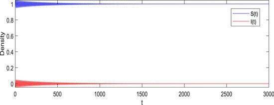
Consider system (4) with the following parameters $b=0.16,\alpha =1.3$, $\sigma =0.8$, $\beta =0.7$ and calculate the basic regeneration number ${R}_{0}=0.729\,2\lt 1$. Therefore, system (4) exists a rumor-free equilibrium point ${E}_{0}=(1,0)$. According to theorem (4.1), system (4) has a Hopf bifurcation at E0 when $\tau ={\tau }_{00}^{0}=1.405\,9$. Hence, as figure 1 shows that the rumor-free equilibrium point E0 is locally asymptotically stable when we choose $\tau =1.40\lt {\tau }_{00}^{0}$. On the other hand, when we take $\tau =1.41\gt {\tau }_{00}^{0},$ the rumor-free equilibrium point E0 is unstable, as shown in figure 2.
Figure 1.
New window|Download| PPT slide Figure 1.The rumor-free equilibrium point E0 is stable when $\tau \lt {\tau }_{00}^{0}$.
Figure 2.
New window|Download| PPT slide Figure 2.The rumor-free equilibrium point E0 is unstable when $\tau \gt {\tau }_{00}^{0}$.
Moreover, as shown in figure 1, as time goes by, the density of transmission users will eventually approach zero and will not fluctuate. This changing trend means that rumors will eventually be wiped out. Furthermore, we can know that system (4) is locally asymptotically stable. Meanwhile, it can be seen from figure 2 that the density of network individuals maintains a fluctuation state. As time goes by, the fluctuation range becomes larger and larger, which means that the density of network individuals is unstable in the process of rumor spreading. This implies that rumors in the system (4) will continue to erupt periodically.
5.2. The stability of the rumor-prevailing equilibrium point ${E}_{1}^{* }$
Take the following parameters $b=0.4,\alpha =1,$$\sigma =0.3,$$\beta =0.78$ in system (4). By calculating, we get the basic regeneration number ${R}_{0}=1.114\,3\gt 1$. Thus, there is a rumor-prevailing equilibrium point ${E}_{1}^{* }=(0.846\,2,0.153\,8)$ in system (4). According to theorem (4.2), system (4) has a Hopf bifurcation at ${E}_{1}^{* }$ when $\tau ={\tau }_{01}^{0}=5.099\,5$. As figures 3(1) and 3(2) show that the rumor-prevailing equilibrium point ${E}_{1}^{* }$ is locally asymptotically stable when we choose $\tau =5.0\lt {\tau }_{01}^{0}$. In addition, when taking $\tau \,=5.1\,\gt {\tau }_{01}^{0}$, the rumor-prevailing equilibrium point ${E}_{1}^{* }$ is unstable, as shown in figures 4(1) and (2).
Figure 3.
New window|Download| PPT slide Figure 3.The rumor-prevailing equilibrium point ${E}_{1}^{* }$ is stable when $\tau \lt {\tau }_{01}^{0}$.
Figure 4.
New window|Download| PPT slide Figure 4.The rumor-prevailing equilibrium point ${E}_{1}^{* }$ is unstable when $\tau \gt {\tau }_{01}^{0}$.
In addition, figure 3 shows that, over time, the density of network individuals converges to a positive number and does not fluctuate again, which implies that rumors will still spread in the social network in a stable state. At the same time, it can be seen from figure 4 that the density of network individuals maintains a fluctuating state, and the range of fluctuations increases with the passage of time, which means that the density of network individuals is unstable and increasing. This suggests that the rumor in system (4) will not be controlled in a certain range and will continue to break out in stages.
5.3. The influence of infectious rate β on rumor propagation
In this section, we analyze the influence of β on rumor propagation by changing the value of β and keeping the other parameters b=0.25, Σ=0.3, α=1, τ=2 unchanged. As is shown in figure 5(1) (β=0.58), figure 6(1) (β=0.63) and figure 7(1) (β=0.67), with the increase of β, the maximum value for the density of rumor transmission users becomes larger. That is to say, the larger the infection rate β, the more widespread the rumor is spreading in social networks. This is consistent with the rumor propagation rules in real social networks.
Furthermore, by comparing the time of reaching stability between system (3) and system (4), we analyze the influence of time delay and nonlinear function on rumor propagation which [28] does not take into account. Without loss of generality, we compare figure 5(1) with figure 5(2), figure 6(1) with figure 6(2), figure 7(1) with figure 7(2), we can find that the time to reach stability of system (4) is shorter than that of system (3). That is to say, when rumors break out, the number of people who spread rumors in system (4) are more likely to be controlled within a certain range than those in system (3). Therefore, the incorporation of nonlinear functions and time delay into the rumor propagation model enriches our understanding of rumor propagation dynamics.
5.4. The influence of cure rate Σ on rumor propagation
In order to study the effect of Σ on rumor propagation, we keep the parameters b=0.25, β=0.58, α=1, τ=2 unchanged and change the value of Σ. It can be seen from figure 8(1) ($\sigma =0.21$), figure 9(1) ($\sigma =0.28$), figure 10(1) ($\sigma =0.31$), with the increase of Σ, the maximum value for the density of rumor transmission users becomes smaller. In other words, the higher the cure rate, the less likely the rumor is to spread in the social network. This is in line with the laws of rumour in the real social network.
The same as in section 5.3, comparing figure 8(1) with figure 8(2), figure 9(1) with figure 9(2), and figure 10(1) with figure 10(2), we can find that the time for system (4) to reach stability is shorter than system (3), which also means that system (4) will be easier to achieve steadiness. In other words, adding time delay and using nonlinear function will make system more quickly to achieve steadiness. This also provides us with ideas to control the rumors more effectively. For example, we can strengthen the intervention on rumor propagation and take certain measures to make the rumor transmission users recover from the rumor more quickly. In this way, rumors in the system can be controlled in a certain range with a shorter time.
6. Conclusion
This paper presents an SIS model of network rumor propagation with nonlinear functions and time delay. Based on the next-generation matrix method, we obtain the basic reproduction number R0. In the following, we give the conditions for judging whether the equilibrium points exist or not. In addition, when ${R}_{0}\lt 1$, there may be multiple rumor-prevailing equilibrium points, which is called the backward bifurcation phenomenon. By analyzing the corresponding characteristic equations of system (4), we obtain the local stability of the equilibrium points. When ${R}_{0}\lt 1$ and f02≥0, the rumor-free equilibrium point E0 is locally asymptotically stable for all $\tau \in [0,+\infty )$. Moreover, if R0>1 and ${f}_{04}\geqslant 0$, the rumor-prevailing equilibrium point ${E}_{1}^{* }$ is locally asymptotically stable for all $\tau \gt 0$. Based on the Hopf bifurcation theory, we obtain the conditions for Hopf bifurcation at E0 and ${E}_{1}^{* }$. If f02<0, system (4) has a Hopf bifurcation at E0 when $\tau ={\tau }_{00}^{0}$. In addition, if R0>1 and f04<0, a Hopf bifurcation occurs at ${E}_{1}^{* }$ when $\tau ={\tau }_{01}^{0}$ in system (4). Last but not least, numerical simulations are carried out to verify the correctness of the above theories. Furthermore, by studying the influence of some parameters on the system, we find that the larger the infection rate β, the more widespread the rumor is spreading in the social network, and the higher the cure rate, the less likely the rumor is to spread in the social network. In addition, we also discover that the addition of time delay and the use of nonlinear function makes the system quicker in achieving steadiness. These studies are still far from enough. In the future, we will continue to consider the influence of other factors, such as more time delay, partial differential equation, media reports and so on, to improve the model, which will make it more realistic.
Acknowledgments
This research is supported by the China Postdoctoral Science Foundation (Grant No.2019M661732), the Natural Science Research of the Jiangsu Higher Education Institutions of China (Grant No.19KJB110001) and the Natural Science Foundation of Jiangsu Province, China (Grant No.BK20190836).
 ,1, Xiaoyuan HuangFaculty of Science,
 New window|Download| PPT slide
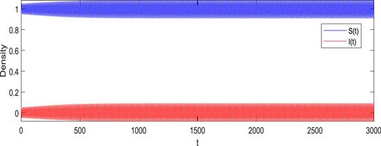 New window|Download| PPT slide
 New window|Download| PPT slide
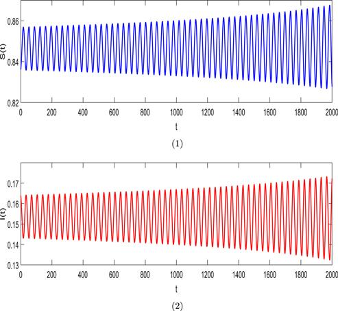 New window|Download| PPT slide
 New window|Download| PPT slide
 New window|Download| PPT slide
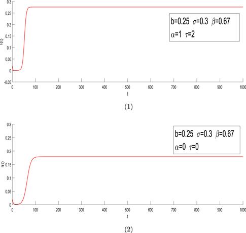 New window|Download| PPT slide
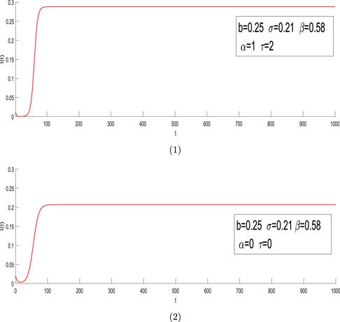 New window|Download| PPT slide
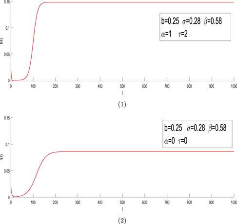 New window|Download| PPT slide
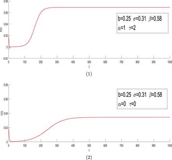 New window|Download| PPT slide