Abstract:Relaxation oscillations are ubiquitous in various fields of natural science and engineering technology. Exploring possible routes to relaxation oscillations is one of the important issues in the study of relaxation oscillations. Recently, the pulse-shaped explosion (PSE), a novel mechanism which can lead to relaxation oscillations, has been reported. The PSE means pulse-shaped sharp quantitative changes related the variation of system parameters in branches of equilibrium points and limit cycles, which leads the system’s trajectory to undertake sharp transitions and further induces relaxation oscillations. Regarding externally and parametrically excited nonlinear systems with different frequency ratios, some work on PSE has been reported. The present paper focuses on the PSE and the related relaxation oscillations in a externally and parametrically excited Mathieu-van der Pol-Duffing system. We show that if there is an initial phase difference between the slow excitations with the same frequency ratio, the fast subsystem may compose of two parts with different expressions, each of which determines a different vector field. As a result, the bistable behaviors are observed in the system. In particular, one of the vector fields exhibits two groups of bifurcation behaviors, which are symmetric with respect to the positive and negative PSE, and each can induce a cluster in the relaxation oscillations. Based on this, we present several routes to compound relaxation oscillations, and obtain new types of relaxation oscillations connected by pulse-shaped explosion, which we call compound “subHopf/fold-cycle” relaxation oscillations and compound “supHopf/supHopf” relaxation oscillations, respectively. Our results show that the two clusters in the resultant relaxation oscillations are connected by the PSE, and the initial phase difference plays an important role in transitions to different attractors and the generation of relaxation oscillations. Although the research in this paper is based on a specific nonlinear system, we would like to point out that the bistable behaviors, the PSE and the resultant compound relaxation oscillations can also be observed in other dynamical systems. The reason is that the fast subsystem composes of two different vector fields induced by the initial phase difference, which dose not rely on a specific system. The results of this paper deepen the research about PSE as well as the complex dynamics of relaxation oscillations. Keywords:relaxation oscillations/ pulse-shaped explosion/ frequency conversion fast-slow analysis/ multi-frequency excitations/ bifurcation mechanism
当系统仅含一个吸引子时, 系统表现出所谓的单稳定性; 而当两个或两个以上吸引子共存时, 便得到了双稳定性或多稳定性[43,44]. 对于本文所考虑的系统来说, 在相位差的作用下, 其快子系统被分解为由方程(2a)和(2b)决定的两个部分. 而每个向量场部分都可能会产生吸引子, 因此相位差的存在可能会诱发快子系统的双稳定性. 为了揭示相位差下的双稳定性, 作出快子系统(2)关于$(w, \alpha )$参数平面的分岔集(见图2), 系统参数的取值与图1相同. 此外, 为了清晰地展示各向量场部分的稳定性和分岔行为, 将分岔集切分为对应于子系统(2a)和(2b)的两个部分, 并分别绘制于图2(a)和图2(b)中. 图 2 (a)子系统(2a)和(b)子系统(2b)在参数平面$(w, \alpha )$上的分岔集. 其中GH为广义Hopf分岔SubH为亚临界Hopf分岔, SupH为超临界Hopf分岔, LPC为极限环的分岔. 系统参数的取值与图1相同 Figure2. Bifurcation sets of the subsystem (2a) (a) and (2b) (b) in the parameter plane $(w, \alpha )$. Here GH represent the generalized Hopf bifurcation, SubH represent the subcritical Hopf bifurcation, SupH represent the supercritical Hopf bifurcation, LPC represent the limit point cycle bifurcation. The values of system parameters are the same as those in Fig. 1.
如图2所示, 参数平面$\left( {w, \alpha } \right)$被直线$\alpha = 0.466$和$\alpha = 0.333$划分为A, B, C三个区域. 首先, 考虑参数$\alpha $属于区域A的情形(即$\alpha > 0.466$). 以$\alpha = 1.5$时的情形为例, 当w从–1开始逐渐增大时(对应图2(a)), 系统仅含唯一的一个吸引子, 即极限环吸引子(见图3(a1)), 且该吸引子无分岔行为的发生. 当w增大到1之后, 便逐渐减小. 此时, 系统从向量场(2a)切换到(2b). 随着w的逐渐减小, w将依次穿越8条分岔曲线, 发生8次分岔(见图3(a2)). 图 3 快子系统(2)在A, B, C各区域中典型的稳定性和分岔行为 (a1), (a2) $\alpha = 1.5$; (b1), (b2) $\alpha = 0.4$; (c1), (c2) $\alpha = 0.2$. 其他参数的取值与图1相同 Figure3. Typical stability and bifurcation behaviors of the fast subsystem (2) in the areas A, B and C: (a1), (a2) $\alpha = 1.5$; (b1), (b2) $\alpha = 0.4$; (c1), (c2) $\alpha = 0.2$. The values of other parameters are the same as those in Fig. 1.
考虑到系统(2b)中, ${\beta _1}$在1附近时存在临界峰值. 为了更加深入地揭示系统的PSE行为, 固定参数$\alpha = 1.5$, 其他系统参数同图1(a). 对转换后的快子系统(2b)作关于$\left( {w, {\beta _1}} \right)$参数平面的分岔集(如图4所示), 的确, 当${\beta _1}$在1附近时系统会产生不同的分岔行为. 为了定性分析快子系统(2b)的分岔行为, 固定其他参数, 仅改变${\beta _1}$, 分别取定${\beta _1}$分别为1.1, 1, 0.99作关于$\left( {w, x} \right)$相平面的分岔图, 如图5(a),图5(b)和图3(a2)所示. 图 4 子系统(2b)在参数平面$\left( {w, {\beta _{\rm{1}}}} \right)$上的分岔集. 其他参数的取值与图1(a)相同 Figure4. Bifurcation sets of the subsystem (2b) in the parameter plane $\left( {w, {\beta _{\rm{1}}}} \right)$. The values of other parameters are the same as those in Fig. 1(a).
图 5 为子系统(2b)的分岔图 (a) ${\beta _1} = 1.1$; (b) ${\beta _1} = 1$. 其他参数的取值与图1(a)相同 Figure5. Bifurcation diagrams of the subsystem (2b): (a) ${\beta _1} = $1.1; (b) ${\beta _1} = 1$. The values of other parameters are the same as those in Fig. 1(a).
由于快子系统被划分为对应于不同动力学行为的三个参数区域, 因此当参数取在不同的区域时可能会产生不同的张弛振荡模式. 本部分探讨复合式subHopf/fold-cycle型张弛振荡, 它与参数$\alpha $取在区域A和B有关. 首先考虑$\alpha $取在区域A的情形, 即情形A. 情形A 为了便于分析, 固定$\gamma = 4$, $\delta = 1$, $\omega = 0.01$, ${\beta _1} = 0.99$, ${\beta _2} = 1$, 图2给出了$\left( {w, \alpha } \right)$参数平面上的分岔集. 如图2所示, 当$\alpha > 0.466$时, 在所考虑的参数间隔内不同的$\alpha $不会产生定性的变化. 因此取定$\alpha = 1.5$为情形A. 通过数值模拟可得到时间历程图, 如图1(a)所示, 在每个周期内, 此时系统表现为: 在两个大幅振荡簇之间存在一个正负双向PSE. 为了更好地揭示该系统的动力学行为, 对系统(1)进行快慢分析并引入转换相图, 令$\cos (\omega t + \theta ) = $$\sin (\omega t) = w$, 由于在该多频激励系统中, 慢变参数均可以用关于w的代数式表示. 从而原系统又可以表示为快子系统(2). 将$\sin (\omega t) = w$作为分岔参数, 在$(w, x)$相平面上作分岔图与慢子系统的转换相图的叠加图, 由于在该多频激励系统中还存在着参数激励$\cos (\omega t)$, 在用含有w的参数表示时, 原系统的分岔图及转换相图应由两部分组成, 如图6所示. 在系统(2)中, $\alpha = 1.5$为对应的情形A. 图 6图1(a)中的张弛振荡的快慢分析 (a)张弛振荡的转换相图与图3(a1)中的分岔图的叠加(与子系统(2a)相关); (b)张弛振荡的转换相图与图3(a2)中分岔图的叠加(与子系统(2b)相关); (c)一个完整周期下的张弛振荡. 这里$\alpha = 1.5$, 而其他参数与图1相同 Figure6. Fast-slow analysis of the relaxation oscillations in Fig. 1(a): (a) Overlay of the transformed phase diagram of the relaxation oscillations and the bifurcation diagram in Fig. 3(a1) (related to the subsystem (2a)); (b) overlay of the transformed phase diagram of the relaxation oscillations and the bifurcation diagram in Fig. 3(a2) (related to the subsystem (2b)); (c) a whole period of the relaxation oscillations. Here $\alpha = 1.5$and other parameters are the same as those in Fig. 1.


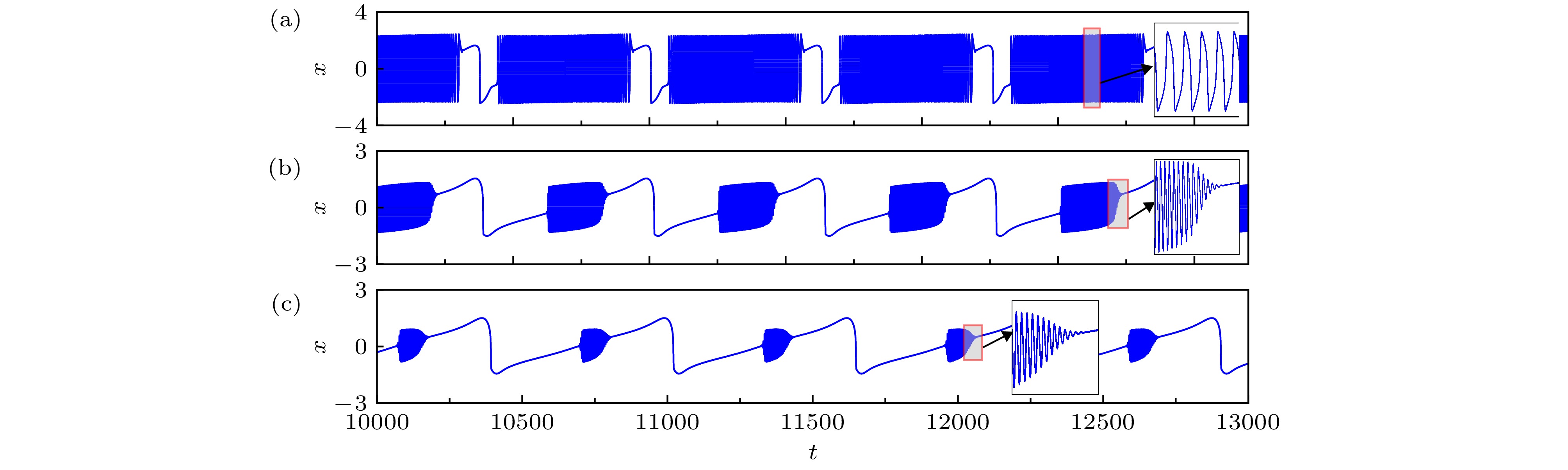 图 1 系统(1)中典型的复合式张弛振荡 (a)


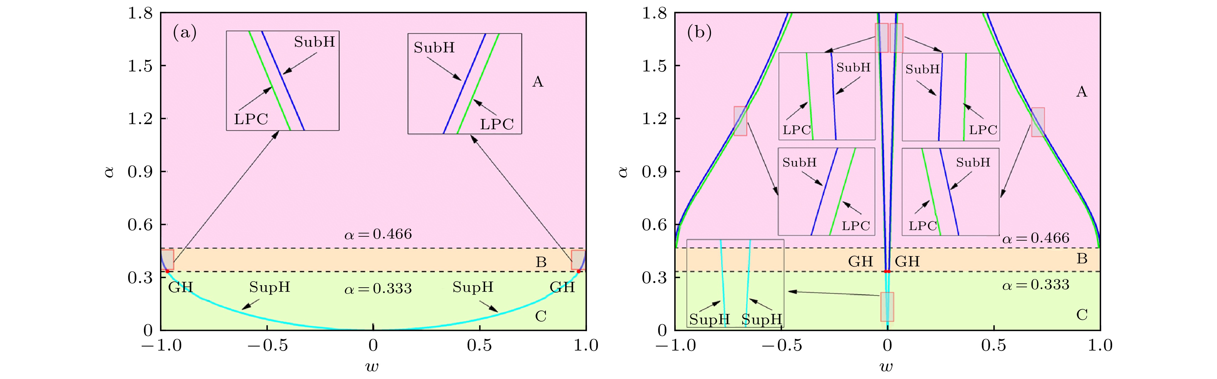 图 2 (a)子系统(2a)和(b)子系统(2b)在参数平面


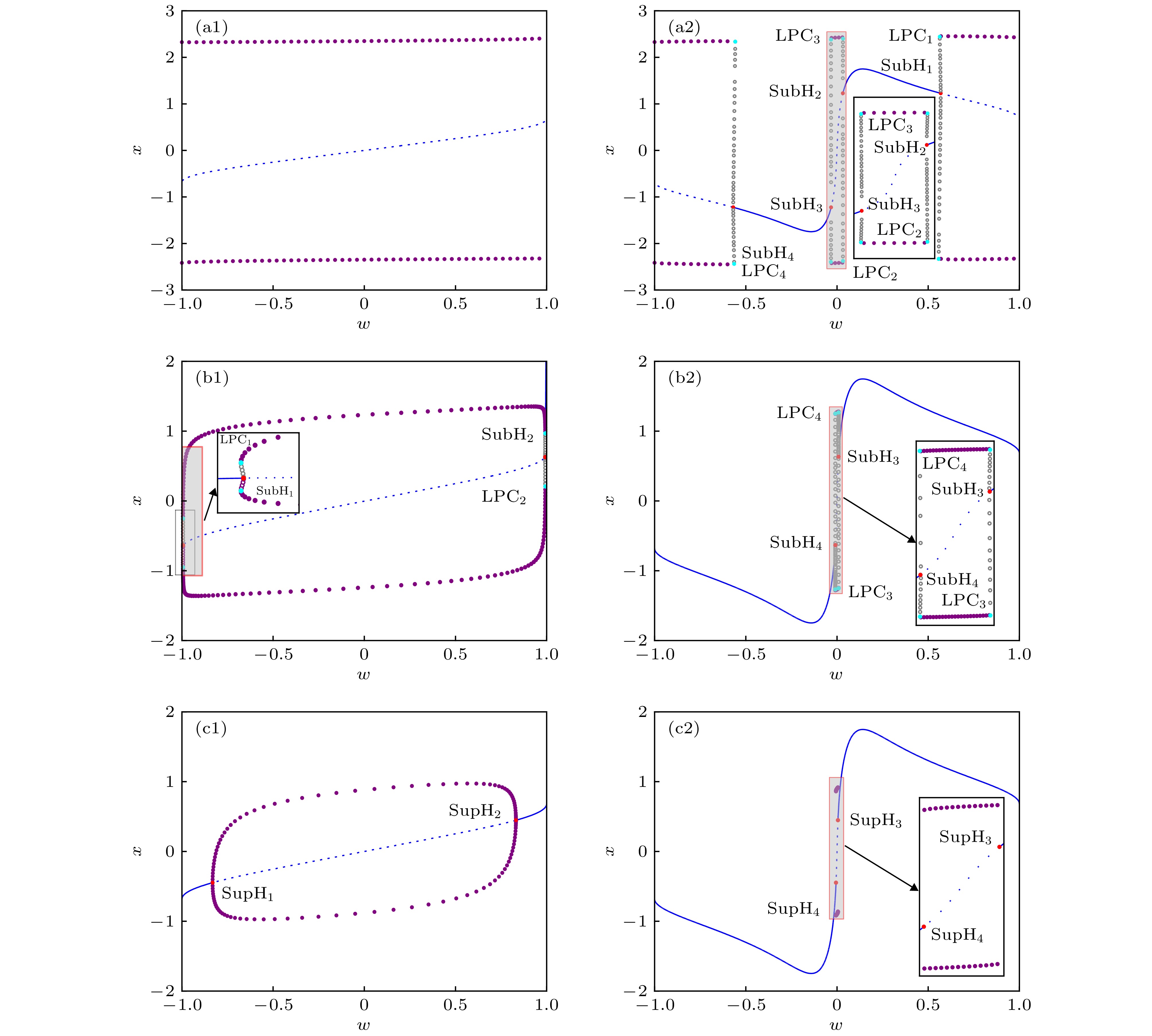 图 3 快子系统(2)在A, B, C各区域中典型的稳定性和分岔行为 (a1), (a2)


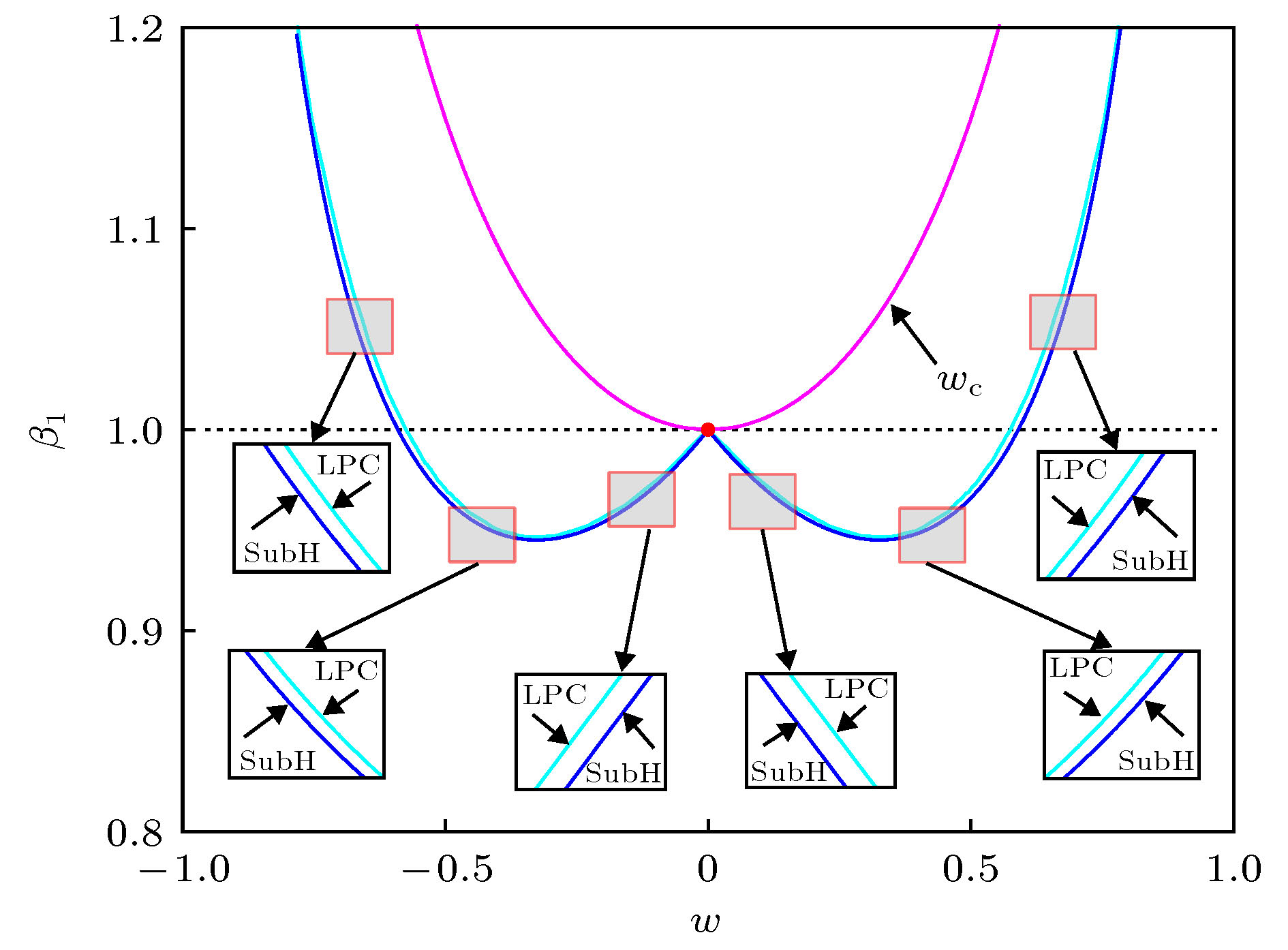 图 4 子系统(2b)在参数平面

 图 5 为子系统(2b)的分岔图 (a)


 图 6 图1(a)中的张弛振荡的快慢分析 (a)张弛振荡的转换相图与图3(a1)中的分岔图的叠加(与子系统(2a)相关); (b)张弛振荡的转换相图与图3(a2)中分岔图的叠加(与子系统(2b)相关); (c)一个完整周期下的张弛振荡. 这里


 图 7 图1(b)中的张弛振荡的快慢分析


 图 8 图1(c)中的张弛振荡的快慢分析