摘要: 利用投影切片定理、傅里叶位移定理和误差函数给出三能级钾原子气体三维傅里叶变换频谱在
T = 0界面的解析解. 固定均匀线宽, 非均匀展宽和对角线相关系数可以定量地识别, 通过在适当方向上拟合三维傅里叶变换频谱谱峰的切片来确定. 结果表明, 非均匀展宽增大, 频谱图沿着对角线方向延伸, 对角线相关系数增大, 频谱图逐渐变圆, 振幅也逐渐变小.
关键词: 傅里叶变换谱 /
四波混频 /
原子气体 English Abstract Analytical solution of three-dimensional Fourier transform frequency spectrum for three-level potassium atomic gas Zhao Chao-Ying 1,2 ,Tan Wei-Han 3 1.School of Sciences, Hangzhou Dianzi University, Hangzhou 310018, China Fund Project: Project supported by the National Natural Science Foundation of China(Grant No. 11504074) and the Key Laboratory of Quantum Optics, Ministry of Education, China (Grant No. KF201801)Received Date: 20 June 2019Accepted Date: 21 October 2019Published Online: 20 January 2020Abstract: With the development of laser technology in the field of optics, ultra-fast optics has become an important research field. Compared with the traditional technology, ultrafast optics can be realized not only under shorter pulse function, but also on a smaller scale, which can more quickly reflect the dynamic process. We present an analytical calculation of the full three-dimensional (3D) coherent spectrum with a finite duration two-dimensional (2D) Gaussian pulse envelope. Our starting point is the solution of the optical Bloch equations for three-level potassium atomic gas in the 3D time domain by using the projection-slice theorem, error function and Fourier-shift theorem of 3D Fourier transform. These principles are used to calculate and simplify the third-order polarization equation generated by the device, and the analytical calculation of three-dimensional Fourier transform frequency spectrum at T = 0 is obtained. We simulate the analytic solution by using mathematics software. By comparing the simulations with the experimental results, with the homogeneous line-width fixed, we can obtain the relationship among the in-homogeneous broadening, the correlation diagonal coefficients and the three-dimensional spectrum characteristics, which can be identified quantitatively by fitting the slices of three-dimensional Fourier transform spectrum peaks in an appropriate direction. The results show that the three-dimensional Fourier transform spectrum will extend along the diagonal direction with the increasing of the in-homogeneous broadening, and the spectrogram progressively becomes a circle with the increasing of the diagonal correlation coefficient, and the amplitude also gradually turns smaller. According to the analytical solution, we give a complete two-dimensional spectrum of the T = 0 interface. The results can be fit to the experimental 3D coherent spectrum for arbitrary inhomogeneity.Keywords: Fourier transform spectrum /four-wave-mixing /atomic gas 全文HTML --> --> --> 1.引 言 基于三脉冲瞬态四波混频技术[1 ] 的多维傅里叶变换光谱学的诞生是超快光谱学的一个重要进展. 多维光谱学的概念最初是从20世纪核磁共振发展起来的[1 ] , 最常见的是二维相干谱[2 ] , 2010年, Siemens等[3 ] 应用投影切片定理首次解析求解了二维傅里叶变换光谱中任意非均匀的对角线和交叉对角线切片共振线型, 其结果可用于实验数据中多个共振的均匀和非均匀展宽的定量测量. 二维光谱具有的特点也使它成为了研究各种结构和动态的重要工具, 例如, 水中的氢键动力学[4 ] 、半导体量子阱[5 -8 ] 的多体动力学等. 2013年, Li等[9 ] 首次在实验上实现了钾原子气体的三维傅里叶变换谱, 该变换谱能清晰地揭示每条路径的跃迁能、弛豫速率和偶极矩. 2015年, Bell等[10 ] 应用投影切片定理首次解析求解了二维傅里叶变换谱. 其结果可用于任意非均匀共振的二维相干谱实验. 二维光谱具有分解不同的量子激发路径的能力, 所以用二维光谱研究碱金属原子体系. 2017年, Titze和Li[11 ] 计算了激发脉冲序列在特定相位匹配方向上的三阶非线性光学响应, 其结果与文献[9 ]在$T = {\rm{0}}$ 截面的实验结果一致. 国内, 清华大学戴星灿课题组[12 -14 ] 使用多维傅里叶光谱的方法对碱金属分子量子系统中的动力学过程进行了详细的研究. 南京大学肖敏课题组[15 ,16 ] 采用超短脉冲, 并在其基础上发展了对抽运的相关探测、时间分辨荧光等超快光谱学方法. 近几年, 陕西师范大学的李晓辉课题组[17 -20 ] 开展了石墨烯等二维材料的非线性光学和超快光子学的研究工作. 考虑到文献[12 ]只给出了钾原子气体三维傅里叶变换谱的数值解, 没有给出频域谱的解析解, 因此, 本文给出了钾原子气体三维傅里叶变换谱在$T = {\rm{0}}$ 截面的解析解, 其结果与文献[9 ,11 ]的数值解一致.2.三维傅里叶变换谱 早期的三维相干光谱的实验[21 ,22 ] 是基于样品对5个激发场的五阶非线性响应的, 但是为了获得更完整的电子跃迁信息, 研究三维光谱时对电子跃迁主要集中在了三阶非线性响应上. 本文选用能级系统简单的碱金属原子蒸气研究三维傅里叶变换谱[12 -14 ] , 如图1 所示.图 1 四波混频原理图Figure1. Four wave mixing schematic.${t_1}$ , ${t_2}$ , ${t_3}$ 时刻分别发射第一个、第二个、第三个脉冲信号, 其中$\tau $ 为第一个脉冲和第二个脉冲之间的时间延迟, T 为第二个脉冲和第三个脉冲之间的时间延迟, t 为发射时间. 四波混频起因于非线性光学中的三阶非线性极化[23 ] , 满足动量守恒${k_4} = {k_1} - {k_2} - {k_3}$ 和能量守恒${\omega _4} \!=\! {\omega _1} \!+\! {\omega _2}+ {\omega _3}$ . 频率为${\omega _4}$ 的光波产生的三阶非线性极化强度为${R^{(3)}}(t_A', t_B', t_C')$ 为三阶非线性响应函数.${H_{ij}} = \hbar {\omega _i}{{\text{δ}} _{ij}} - {\mu _{ij}}E(t)$ , $\hbar {\omega _i}$ 为i 态的能量, ${\mu _{ij}}$ 为i , j 两能级跃迁电偶极矩; 弛豫算符$\varGamma $ 的矩阵元${\varGamma _{ij}} = {{\rm{1}} / {\rm{2}}}({\gamma _i} + {\gamma _j})$ , ${\gamma _i}$ , ${\gamma _j}$ 为i , j 能级能级的布居数衰减率.[11 ] :$T = {\rm{0}}$ 时, A 路径为[11 ] $t' = t + \tau $ 为时域中的对角线方向, $\tau ' = t - \tau $ 为时域中的交叉对角线方向[3 ] . 通过时域中对交叉对角线上的投影进行傅里叶变换来计算频域中交叉对角线的切片, 称之为投影切片定理[10 ] . 也就是说, 切片沿着${\omega _{{t'}}}$ , 位移沿着${\omega _{{\tau '}}}$ ; 切片沿着${\omega _{{\tau '}}}$ , 位移沿着${\omega _{{t'}}}$ . 二维频域沿${\omega _x}$ 方向上的位移$\Delta {\omega _x}$ 相当于在二维时域中乘以${{\rm{e}}^{ - {\rm{i}}\Delta {\omega _x}t}}$ , 如图2 所示.图 2 (a) 二维时域; (b) 光子回波信号的频率坐标; (c) 二维时域投影在对应于沿${\hat \omega _{{t'}}}$ 的切片的对角线上; (d)沿${\hat \omega _{{\tau '}}}$ 的切片对应的交叉对角线上的二维时域投影Figure2. (a) 2D time; (b) frequency coordinates for photon echo signals; (c) 2D time projection onto the diagonal corresponding to a slice along ${\hat \omega _{{t'}}}$ ; (d) 2D time projection onto the cross diagonal corresponding to a slice along ${\hat \omega _{{\tau '}}}$ .A 路径[11 ] 下对应的三阶非线性极化方程形式简化如下:${\varGamma _{10}}$ 和${\varGamma _{{\rm{2}}0}}$ , 非均匀线宽为${\text{δ}} {\omega _{10}}$ 变为${\text{δ}} {\omega _{20}}$ .A 路径[10 ] 下对应的频域形式为[10 ] :A 路径下对应的频域谱的解析解为${\text{δ}} {\omega _{10}}$ 变为${\text{δ}} {\omega _{20}}$ , 将${\varGamma _{10}}$ 变为${\varGamma _{{\rm{2}}0}}$ , 就是B 路径的解析结果[11 ] .11 ], C -F 路径中含有$t\tau $ 交叉项, 时域的解析解可简写为$x = {\text{δ}} \omega _{10}^2 - 2 R{\text{δ}} {\omega _{{\rm{10}}}}{\text{δ}} {\omega _{{\rm{20}}}} + {\text{δ}} \omega _{20}^2$ , $y = {\text{δ}} \omega _{10}^2 + $ $ 2 R{\text{δ}} {\omega _{{\rm{10}}}}{\text{δ}} {\omega _{{\rm{20}}}} + {\text{δ}} \omega _{20}^2$ , $z = {\text{δ}} \omega _{20}^2 - {\text{δ}} \omega _{10}^2$ . $\varTheta $ 是Heaviside阶跃函数. 考虑到C -F 路径含有$t\tau $ 这一交叉项, 在化简时无法将其分离, 同时系数R 存在, 使得计算过程相较A , B 两路径更为复杂, 因此, 将${\text{δ}} {\omega _{10}}$ 与${\text{δ}} {\omega _{20}}$ 的比值定义为m , 如表1 所示.x y z ${\text{δ}} {\omega _{10}} = {\text{δ}} {\omega _{20}}$, $R = {\rm{1}}$ 0 ${\rm{4}}{\text{δ}} \omega _{10}^2$ 0 ${\text{δ}} {\omega _{10}} = {\text{δ}} {\omega _{20}}$, $R \ne {\rm{1}}$ $2\left( {1 - R} \right){\text{δ}} \omega _{10}^2$ $2\left( {{\rm{1}} + R} \right){\text{δ}} \omega _{10}^2$ 0 ${\text{δ} } {\omega _{10} } = m{\text{δ} } {\omega _{20} },$$R = {\rm{1}}$ ${\left(1 - \dfrac{1}{m}\right)^2}{\text{δ}} \omega _{10}^2$ ${\left(1 + \dfrac{1}{m}\right)^2}{\text{δ}} \omega _{10}^2$ $\left(1- \dfrac{1}{{{m^2}}}\right){\text{δ}} \omega _{10}^2$ ${\text{δ} } {\omega _{10} } = m{\text{δ} } {\omega _{20} },$$R \ne {\rm{1}}$ $\dfrac{{({m^2} - 2 Rm + 1)}}{{{m^2}}}{\text{δ}} \omega _{10}^2$ $\dfrac{{({m^2} + 2 Rm + 1)}}{{{m^2}}}{\text{δ}} \omega _{10}^2$ $\left(1 - \dfrac{1}{{{m^2}}}\right){\text{δ}} \omega _{10}^2$
表1 非均匀展宽和对角线相关系数之间的关系Table1. The relation between in-homogeneous line-width and the diagonal correlation coefficient.${\text{δ}} {\omega _{10}} = {\text{δ}} {\omega _{20}}$ , $R = {\rm{1}}$ 时, 频域谱${S_{C{\rm{1}}}}\left( {{\omega _t}, {\omega _\tau }} \right)$ , ${S_{D{\rm{1}}}}\left( {{\omega _t}, {\omega _\tau }} \right)$ , ${S_{E{\rm{1}}}}\left( {{\omega _t}, {\omega _\tau }} \right)$ , ${S_{F{\rm{1}}}}\left( {{\omega _t}, {\omega _\tau }} \right)$ 能够得到和A 路径(7 )式一致的解析解.${\text{δ}} {\omega _{10}} = {\text{δ}} {\omega _{20}}$ , $R \ne {\rm{1}}$ 时, 频域谱的解析解变为${\text{δ}} {\omega _{10}} = {\text{δ}} {\omega _{20}}$ , 所以频域谱${S_{D{\rm{2}}}}\left( {{\omega _t}, {\omega _\tau }} \right)$ , ${S_{E{\rm{2}}}}\left( {{\omega _t}, {\omega _\tau }} \right)$ , ${S_{F{\rm{2}}}}\left( {{\omega _t}, {\omega _\tau }} \right)$ 能够得到和C 路径一致的解析解.${\text{δ}} {\omega _{10}} = m{\text{δ}} {\omega _{20}}$ , $R = {\rm{1}}$ 时, 频域谱的解析解为${\text{δ}} {\omega _{10}} = m{\text{δ}} {\omega _{20}}$ , $R \ne {\rm{1}}$ 时, 频域谱的解析解为${\text{δ}} {\omega _{10}}$ 变为${\text{δ}} {\omega _{20}}$ , E , F 分别与C , D 路径的解析解一致.10 )—(17 )式中可以看出, 路径差别仅仅与$\varGamma $ 和${\text{δ}} \omega $ 有关. 接下来, 通过数值模拟观察$\varGamma $ 和${\text{δ}} \omega $ 分别对光谱的影响.3.数值模拟 数值模拟中, 取如下参数: ${\omega _{10}} = 386 \;{\rm{THz}}$ , ${\omega _{20}} = 388\;{\rm{THz}}$ . 根据(9 ), (10 )式, 路径A 不含对角线相关系数R 的交叉项, B 路径所得三维傅里叶变换频谱图与A 路径的图是一样的. 根据(11 ), (12 )式, 路径C -F 含对角线相关系数R 的交叉项. 比较图3 和图4 , 固定$m = {\rm{1}}.{\rm{5}}$ , 改变R , 随着R 的减小, ${S_{C2}}\left( {{\omega _t}, {\omega _\tau }} \right)$ 谱形逐渐变圆, 振幅逐渐变小. 比较图3 和图5 , 当$R = 1$ 时, 即对角线相关系数相同, m 的变化可以看作是非均匀线宽的变化, 随着m 的减小, ${S_{C3, E{\rm{3}}}}\left( {{\omega _t}, {\omega _\tau }} \right)$ 谱线范围向两边延长, 频谱图变细长. 比较图4 和图6 , 改变非均匀线宽, 随着m 的减小, ${S_{C4, E4}}\left( {{\omega _t}, {\omega _\tau }} \right)$ 谱线范围向两边延长, 频谱图变细长. 比较图5 和图6 , 改变对角线相关系数, ${S_{C4, E4}}\left( {{\omega _t}, {\omega _\tau }} \right)$ 图像变得更圆.图 3 当${\text{δ}} {\omega _{10}} = {\text{δ}} {\omega _{20}} = 0.2\;{\rm{ THz}}$ , ${\varGamma _{10}} = {\varGamma _{{\rm{2}}0}} = 0.05\;{\rm{THz}}$ , $R = 1$ 时${S_{C{\rm{1}}}}\left( {{\omega _t}, {\omega _\tau }} \right)$ 频谱图 (a)实部; (b)虚部; (c)模Figure3. The three-dimensional Fourier transform spectrum ${S_{C{\rm{1}}}}\left( {{\omega _t}, {\omega _\tau }} \right)$ with ${\text{δ}} {\omega _{10}} = {\text{δ}} {\omega _{20}} = 0.2\;{\rm{ THz}}$ , ${\varGamma _{10}} = {\varGamma _{{\rm{2}}0}} = 0.05\;{\rm{THz}}$ , $R = 1$ : (a) Real part; (b) imaginary part; (c) module.图 4 当${\text{δ}} {\omega _{10}} = {\text{δ}} {\omega _{20}} = 0.2\;{\rm{THz}}$ , ${\varGamma _{10}} = {\varGamma _{{\rm{2}}0}} = 0.05\;{\rm{THz}}$ , $R = 0.5$ 时${S_{C2}}\left( {{\omega _t}, {\omega _\tau }} \right)$ 频谱图 (a)实部; (b)虚部; (c)模Figure4. The three-dimensional Fourier transform spectrum ${S_{C2}}\left( {{\omega _t}, {\omega _\tau }} \right)$ with ${\text{δ}} {\omega _{10}} = {\text{δ}} {\omega _{20}} = 0.2\;{\rm{ THz}}$ , ${\varGamma _{10}} = {\varGamma _{{\rm{2}}0}} = 0.05\;{\rm{THz}}$ , $R = 0.5$ : (a) Real part; (b) imaginary part; (c) module.图 5 当${\text{δ}} {\omega _{10}} = 0.3\;{\rm{THz}}$ , ${\text{δ}} {\omega _{20}} = 0.2\;{\rm{THz}}$ , ${\varGamma _{10}} = {\varGamma _{{\rm{2}}0}} = 0.05 \;{\rm{THz}}$ , $R = 1$ 时${S_{C3, E{\rm{3}}}}\left( {{\omega _t}, {\omega _\tau }} \right)$ 频谱图 (a)实部; (b)虚部; (c)模Figure5. The three-dimensional Fourier transform spectrum ${S_{C3, E{\rm{3}}}}\left( {{\omega _t}, {\omega _\tau }} \right)$ with ${\text{δ}} {\omega _{10}} = 0.3\;{\rm{THz}}$ , ${\text{δ}} {\omega _{20}} = 0.2\;{\rm{THz}}$ , ${\varGamma _{10}} = {\varGamma _{{\rm{2}}0}} = $ 0.05 THz, $R = 1$ : (a) Real part; (b) imaginary part; (c) module.图 6 当${\text{δ}} {\omega _{10}} = 0.3\;{\rm{THz}}$ , ${\text{δ}} {\omega _{20}} = 0.2\;{\rm{THz}}$ , ${\varGamma _{10}} = {\varGamma _{{\rm{2}}0}} = 0.05\;{\rm{THz}}$ , $R = 0.5$ 时${S_{C4, E4}}\left( {{\omega _t}, {\omega _\tau }} \right)$ 频谱图 (a)实部; (b)虚部; (c)模Figure6. The three-dimensional Fourier transform spectrum ${S_{C4, E4}}\left( {{\omega _t}, {\omega _\tau }} \right)$ with ${\text{δ}} {\omega _{10}} = 0.3\;{\rm{THz}}$ , ${\text{δ}} {\omega _{20}} = 0.2\;{\rm{THz}}$ , ${\varGamma _{10}} = {\varGamma _{{\rm{2}}0}} = $ 0.05 THz, $R = 0.5$ (a) Real part; (b) imaginary part; (c) module.${\varGamma _{10}}$ , ${\varGamma _{20}}$ , 与非均匀展宽相关的参数R , m , ${\text{δ}} {\omega _{10}}$ , ${\text{δ}} {\omega _{20}}$ 可以定量地识别, 通过在适当方向上拟合三维谱峰的切片来确定[3 ] . 为了能更清楚地观察到对角峰和非对角峰随着参数的变化而发生的变化, 将A -F 路径的频谱图画在一张图中, 进一步得到$T = {\rm{0}}$ 界面完整的三维傅里叶变换频谱图. 如图7 、图8 所示, 左上角为A 路径模的图谱, 右下角为B 路径模的图谱, 右上角为C 路径模的图谱, 左下角为D 路径模的图谱, 根据(13 )式和(15 )式, E 路径所得三维傅里叶变换频谱图与C 路径的图是一样的. 根据(14 )式和(16 )式, F 路径所得三维傅里叶变换频谱图与D 路径的图是一样的. 这样就得到了$T = {\rm{0}}$ 界面各个路径完整的截面图. 但是对于A , B 两条路径来说, 改变对角线相关系数并不会影响它们的图谱, 由于A , B 两路径的频谱图位于整体图的对角峰位置, 对角峰不受R 的影响, 因为它们是由单一的跃迁分别决定的. C , D 两路径的频谱图位于整体图的非对角峰位置, 非对角峰会受到R 的影响, 因为非对角峰与两个跃迁都有关系, 因此受到它们之间相关性的影响. 比较图7(a) 和图(b) , 得到的结果与参考文献[11 ]里的图5(a) 完全一致.图 7 三维傅里叶转换频谱图 (a) 参考文献[11 ]中的图5(a) , ${\varGamma _{10}} = {\varGamma _{{\rm{2}}0}} = 0.05 \;{\rm{THz}}$ , ${\text{δ}} {\omega _{10}} = {\text{δ}} {\omega _{20}} = 0.2\;{\rm{THz}}$ , (b)$R = 1$ ; (c)$R = 0.5$ Figure7. Three-dimensional Fourier transform spectrum: (a) Fig. 5(a) in Ref. [11 ], ${\varGamma _{10}} = {\varGamma _{{\rm{2}}0}} = 0.05 \;{\rm{THz}}$ , ${\text{δ}} {\omega _{10}} = {\text{δ}} {\omega _{20}} = $ 0.2 THz; (b)$R = 1$ ; (c)$R = 0.5$ .图 8 R 不同时, 三维傅里叶转换频谱, ${\varGamma _{10}} = {\varGamma _{{\rm{2}}0}} = 0.05\;{\rm{THz}}$ , ${\text{δ}} {\omega _{10}} = 0.3\;{\rm{THz}}$ , ${\text{δ}} {\omega _{20}} = 0.2\;{\rm{THz}}$ (a)$R = 1$ ; (b)$R = 0.5$ Figure8. The three-dimensional Fourier transform spectrum with ${\varGamma _{10}} = {\varGamma _{{\rm{2}}0}} = 0.05\;{\rm{THz}}$ , ${\text{δ}} {\omega _{10}} = 0.3\;{\rm{THz}}$ , ${\text{δ}} {\omega _{20}} = 0.2\;{\rm{THz}}$ for different R : (a) $R = 1$ ; (b) $R = 0.5$ .图7(b) 和图8(a) , 频谱图会随着非均匀线宽的增大而沿对角线方向有一定的延伸, 对角峰的图谱也伸长了, 一般来说, A , B 两路径对应跃迁的非均匀线宽不相等, 对角峰在对角方向上具有不同的线宽, C , D 两路径图谱对应的延伸较为明显.4.结 论 首先利用投影切片定理对三能级钾原子气体三维傅里叶变换谱进行降维; 其次利用误差函数将三阶非线性极化方程进行简化, 傅里叶位移理论将谱从时域转换到频域, 研究了三能级钾原子气体三维傅里叶变换谱与非均匀线宽、对角线相关系数R 和m 之间的关系. 改变R , 随着R 的减小, 谱形逐渐变圆, 振幅逐渐变小. 改变m , 随着m 的减小, 频谱图变细长. 最后, 将A-F 路径的三维傅里叶变换频谱图画在一张图中, 得到$T = {\rm{0}}$ 界面的完整的三维傅里叶变换频谱图. 其解析解与文献[11 ]的图5(a) 数值模拟图完全吻合. 三维光谱中光谱峰的线形显示了非均匀展宽的重要性信息, 通过对角峰的伸长表明存在非均匀展宽, 两个跃迁的相对非均匀线宽由对应的对角线峰值的对角线宽揭示. 此研究结果可进一步推广至任意截面的情况, 最终给出三维光谱的完整的三维图. 这有助于构建一套完整的体系来解释三维傅里叶频谱. 

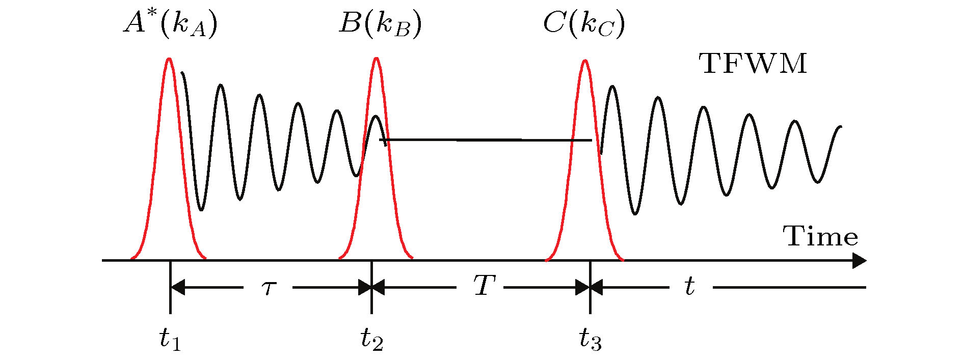 图 1 四波混频原理图


 图 2 (a) 二维时域; (b) 光子回波信号的频率坐标; (c) 二维时域投影在对应于沿


 图 3 当
图 3 当


 图 4 当
图 4 当


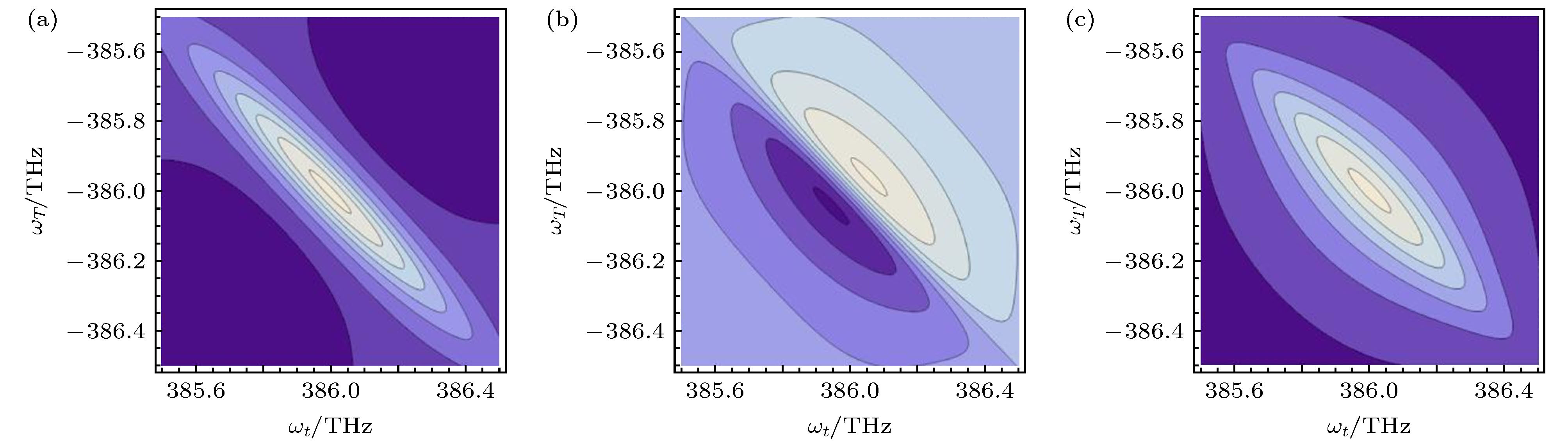 图 5 当
图 5 当


 图 6 当
图 6 当


 图 7 三维傅里叶转换频谱图 (a) 参考文献[11]中的图5(a),


 图 8 R不同时, 三维傅里叶转换频谱,


