于要杰^*,**, 刘锋^†, 高超^*, 冯毅^,**,2)*西北工业大学航空学院, 西安 710072
^†加州大学尔湾分校机械与航天工程系, 美国加利福尼亚州 92697-3975
^**成都流体动力创新中心, 成都 610071

AN IMPLICIT BLOCK JACOBI APPROACH FOR HIGH-ORDER FLUX RECONSTRUCTION METHOD¹⁾

Yu Yaojie^*,**, Liu Feng^†, Gao Chao^*, Feng Yi^,**,2)*Department of Fluid Mechanics, Northwestern Polytechnical University, Xi'an 710072, China
^†Department of Mechanical and Aerospace Engineering, University of California, Irvine, CA 92697-3975, USA
^**Chengdu Fluid Dynamics Innovation Center, Chengdu 610071, China

通讯作者: 2)冯毅, 副研究员, 主要研究方向: 飞行器设计, 计算流体力学. E-mail:fengyi0218@163.com

收稿日期:2020-11-30接受日期:2021-05-13网络出版日期:2021-06-18

基金资助:

1)国家重点研发计划资助项目.2018YFB1501102

Received:2020-11-30Accepted:2021-05-13Online:2021-06-18
作者简介 About authors


摘要
最近, 基于非结构网格的高阶通量重构格式(flux reconstruction, FR)因其构造简单且通用性强而受到越来越多人的关注. 但将FR格式应用于大规模复杂流动的模拟时仍面临计算开销大、求解时间长等问题. 因此, 亟需发展与之相适应的高效隐式求解方法和并行计算技术. 本文提出了一种基于块Jacobi迭代的高阶FR格式求解定常二维欧拉方程的单GPU隐式时间推进方法. 由于直接求解FR格式空间和隐式时间离散后的全局线性方程组效率低下并且内存占用很大. 而通过块雅可比迭代的方式, 能够改变全局线性方程组左端矩阵的特征, 克服影响求解并行性的相邻单元依赖问题, 使得只需要存储和计算对角块矩阵. 最终将求解全局线性方程组转化为求解一系列局部单元线性方程组, 进而又可利用LU分解法在GPU上并行求解这些小型局部线性方程组. 通过二维无黏Bump流动和NACA0012无黏绕流两个数值实验表明, 该隐式方法计算收敛所用的迭代步数和计算时间均远小于使用多重网格加速的显式Runge-Kutta格式, 且在计算效率方面至少有一个量级的提升.
关键词： 高精度格式;通量重构格式;隐式时间推进方法;块雅可比迭代;GPU计算

Abstract
Recently, the flux reconstruction (FR) method has attracted more and more attentions for its simplicity and generality. However, it is still computationally expensive and time consuming when simulating the complex flow problems by FR method. There is a huge demand for developing appropriate efficient implicit solvers and parallel computing techniques for FR. This paper proposes an implicit high-order flux reconstruction solver on GPU platform based on the block Jacobi iteration method. As it is inefficient to solve the large global linear system resulting from spatial and implicit temporal discretization of FR directly. A block Jacobi approach is used to change the characteristics of the lift-hand matrix of the global linear system and this avoids the dependence of neighboring elements. Therefore, only the diagonal blocks of global matrix need to be stored and calculated. Then, the problem of solving the huge global linear system is transformed into solving a series of local linear equations simultaneously. Finally, these small local linear equations would be solved by the LU decomposition method in parallel on GPU platforms. Two typical cases, including subsonic flows over a bump and a NACA0012 airfoil, were simulated and compared with the multi-grid explicit Runge-Kutta scheme. The numerical results demonstrated that the present implicit method can reduce the iterations significantly. Meanwhile, the implicit solver has shown at least 10x speedup over the multi-grid Runge-Kutta scheme in all cases.
Keywords：high-order methods;flux reconstruction method;implicit time-marching methods;block Jacobi iteration;GPU computing


PDF (709KB)元数据多维度评价相关文章导出EndNote|Ris|Bibtex收藏本文
本文引用格式
于要杰, 刘锋, 高超, 冯毅. 一种基于块雅可比迭代的高阶FR格式隐式方法¹⁾. 力学学报, 2021, 53(6): 1586-1598 DOI:10.6052/0459-1879-20-404
Yu Yaojie, Liu Feng, Gao Chao, Feng Yi. AN IMPLICIT BLOCK JACOBI APPROACH FOR HIGH-ORDER FLUX RECONSTRUCTION METHOD¹⁾. Chinese Journal of Theoretical and Applied Mechanics, 2021, 53(6): 1586-1598 DOI:10.6052/0459-1879-20-404

引言

高阶精度数值格式因其高分辨率、低色散和低耗散等特点正日益受到关注^[1-2]. 相比目前工业界最常用的二阶精度格式, 高阶精度格式被认为在花费相同计算代价的前提下具备获得更高精度数值结果的巨大潜力. 当前最常见的高阶精度数值格式主要包括基于结构网格的高阶有限差分方法^[3-4]、非结构网格上的有限体积法^[5-6]以及基于局部单元近似的间断有限元(discontinuous Galerkin, DG)^[7-8]、谱体积(spectral volume, SV)^[9]和谱差分(spectral difference, SD)^[10]等方法.

最近, 一种基于非结构网格的高阶精度通量重构格式(flux reconstruction, FR)因其构造简单且更加通用而愈加流行. FR格式最先于2007年由Huynh^[11-12]提出并证明了, 至少对于一维线性方程, FR格式通过不同修正多项式的选择, 不仅囊括了DG和SD这两种格式, 并且能够产生新的高阶格式. 2009年, Wang和Gao等^[13]提出 "lifting collocation penalty, LCP"格式并将其推广到欧拉方程和Navier-Stokes方程. 由于FR和LCP这两种格式具有高度的相似性和内在联系, 因此后来也被Huynh和王志坚^[14]联合命名为FR/CPR (correction procedure via reconstruction)格式. 2011年, Vincent等^[15]提出了一种针对一维线性对流方程的能量稳定的FR格式, 即VCJH格式, 后续又在此格式的基础上开发了三维并行CFD求解器HiFiLES^[16]和PyFR^[17]. 如今, FR已不仅是一种高阶格式, 它还为几种现有的高阶格式, 例如SD和DG, 提供了一个统一的框架. 相比DG和SD的原有形式, FR在概念上更加简单且计算效率更高^[18]. 关于FR和DG间的联系, Allaneau和Jameson^[19]和De Grazia等^[20]已经进行了深入研究.

尽管FR格式已经取得了较大的进步, 但将其应用于复杂外形流动的数值模拟时, 仍然有一些难点问题需要解决, 例如计算效率的问题、曲面边界处理方法、间断侦测方法与限制器的构造等. 其中, 计算效率的问题在很大程度上制约了FR格式在实际工程中的应用. 在当前的FR格式应用中, 时间离散多采用存储需求小且易实现的显式Runge-Kutta类方法^[21]. 但随着格式精度的提高, FR对应的CFL稳定性条件越来越严格, 时间推进步长会受到明显的限制. 对一些复杂流动问题(流场中存在边界层、剪切层等小尺度流动结构)的计算更是如此. 因此, 发展FR格式的加速收敛方法, 具有十分重要的工程应用价值. 目前常用的加速收敛方法在算法层面主要有隐式时间推进方法、当地时间步长、残差光顺、多重网格以及物理层面的并行计算技术等. 在这些方法中, 隐式时间推进方法的加速效果是十分明显的^[22]. 相比显式时间方法, 隐式方法受CFL稳定性条件的约束小, 可以选取更大的时间推进步长, 进而能够有效地提高CFD求解的效率. 近年来已有****提出了多种基于FR格式的隐式时间方法, 例如LU-SGS方法^[23]、预处理GMERS方法^[24]、无矩阵(Jacobian-free) Newton Krylov方法^[25]以及多色高斯-赛德尔(multi-colored Gauss Seidel, MCGS)方法^[26]等. 这些文章中以数值实验证明, 使用隐式方法的FR格式相比显式具有非常明显的计算效率提升. 以上这些隐式时间方法大都是在CPU架构上实现, 由于基于局部单元近似的FR格式的绝大多数操作都是在局部单元中进行, 计算量较为集中, 因此更适合GPU计算. 当前, 基于CPU并行策略的有限体积求解器一般只能使用并行集群性能峰值的5% $\sim$ 10%, 而使用GPU计算的FR格式计算速度最高可以达到性能峰值的58%左右^[27]. 因此, 基于GPU并行的隐式时间推进方法有望进一步提高FR格式的计算效率.

近年来, GPU计算在CFD领域中的应用已经越来越普遍. 已有的研究结果表明^[27-29], 对于相同规模的问题, GPU并行能够较大程度地提升高阶CFD程序的计算效率. 例如, Romero等^[30]利用显式时间方法的VCJH格式计算非定常流动问题, 发现GPU并行相比基于MPI并行的CPU节点具有更高的计算效率. Vermeire等^[31]使用PyFR求解器在多个GPU卡上以三维Taylor-Green涡和SD7003翼型为例进行隐式大涡模拟计算, 发现与使用CPU节点并行的商业CFD软件Star-CCM+相比, 在计算成本相当的前提下, 5阶FR计算得到的模拟结果更精细. 最近, Jourdan和Wang等^[32]在美国"Summit"超级计算机上使用FR/CPR高阶求解器, 分别利用了800个节点的CPU和4800个GPU卡进行了大涡模拟计算, 发现使用显式时间推进方法时, 在六面体和四面体这两种网格单元类型上, GPU相比CPU并行分别有一个和两个量级左右的加速效果.

在上述的大规模CFD数值模拟中, 基于FR格式的GPU计算使用的都为显式时间方法. 为了探索如何进一步提高FR格式的求解效率, 本文以二维欧拉方程为例, 提出一种基于高阶FR格式的单GPU并行隐式时间求解方法. 通过块Jacobi迭代的方式, 改变了经过隐式离散后全局线性方程组左端矩阵的特征, 克服了影响求解并行性的相邻单元依赖. 最终, 将解全局线性方程组转化解一系列局部单元线性方程组, 进而又通过LU分解法并行求解这些局部线性方程组. 数值实验表明, 相比显式方法而言, 该隐式方法在计算效率方面至少有一个量级的提升. 并且, 该隐式方法不局限于FR格式, 对DG和SD等基于局部单元近似的高阶格式也具有参考意义.

1 控制方程

无黏流动的控制方程为欧拉方程, 其二维形式如下

(1)$\dfrac{\partial { U}}{\partial t} + \dfrac{\partial { F}}{\partial x} + \dfrac{\partial { G}}{\partial y} = {\bf0}$
其中, ${ U}=[\rho , \rho u, \rho v, \rho E]$为守恒变量, ${ F}$和${ G}$分别为$x$和$y$方向的无黏通量

(2)${ F}={ \left[ \begin{array}{c} \rho u \\ \rho u^{2}+p \\ \rho u v\\ u (\rho E+p) \\ \end{array} \right ]}, \quad { G}={ \left[ \begin{array}{c} \rho v\\ \rho v u \\ \rho v^{2}+p\\ v (\rho E+p)\\ \end{array} \right ]}$
式中, $\rho $是密度, $u$和$v$分别表示$x$和$y$方向的速度, $p$为压强, $E$代表单位质量流体的总能量。本文中假设流体为理想气体, 则有

(3)$p = (\gamma -1) \left[ \rho E - \rho (u^{2}+v^{2})/2\right]$
其中, $\gamma=C_{p}/C_{v}$为比热容比, 本文中其值为1.4.

2 高阶通量重构格式

本节将以二维标量守恒律为例来简要地介绍FR格式的基本思想. 在区域$\varOmega \in \mathbb{R}^2$上的一般形式的二维标量守恒律形式为

(4)$\dfrac{\partial u}{\partial t} + \nabla_{xy} \cdot { f } = 0$
其中, $u=u(x, y, t)$为标量守恒量, ${ f }= (f, g)$为通量项, $f=f(u)$和$g=g(u)$分别为${ f }$在$x$和$y$方向的分量.

下面将区域$\varOmega $分割为$N$个互不重叠的四边形子区域$\{\varOmega _{n}\}|^N_{n=1}$, 且子区域满足如下条件

(5)$\bigcup_{n=1}^{N} \varOmega _{n} = \varOmega , \ \ \bigcap_{n=1}^{N}\varOmega _{n}=\emptyset$
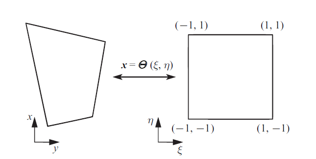
为了数学书写的方便以及计算效率方面考虑, 首先通过如图1所示的变换将物理域$(x, y)$上任意$\varOmega _{n}$转换到计算域$(\xi, \eta)$上的一个标准单元$\varOmega _S$ (为了叙述简洁, 下面将省略下标$n$).

图1

新窗口打开|下载原图ZIP|生成PPT
图1将任意四边形单元变换到一个标准单元

Fig.1Mapping of an arbitrary physical space quadrilateral element to the standard reference quadrilateral element



经过以上变换后, 子区域$\varOmega _{n}$上的方程(4)变换为

(6)$\dfrac{\partial \hat{u}}{\partial t} + \nabla_{\xi \eta} \cdot \hat{{ f }} = 0$
其中, 顶标" $\hat{\ }$ "代表其为计算域$(\xi, \eta)$上的变量, 计算域$(\xi, \eta)$和物理域$(x, y)$上的变量存在如下关系

(7)$\hat{u}(\xi, \eta, t) = Ju( \varTheta(\xi, \eta), t), \ \ J = \dfrac{\partial x}{\partial \xi} \dfrac{\partial y}{\partial \eta} - \dfrac{\partial x}{\partial \eta} \dfrac{\partial y}{\partial \xi}$
(8)$\hat{{ f }}(\xi, \eta, t) = (\hat{f}, \hat{g}) = (\dfrac{\partial y}{\partial \eta}f -\dfrac{\partial x}{\partial \eta}g, \dfrac{\partial x}{\partial \xi}g - \dfrac{\partial y}{\partial \xi}f )$
上述方程(6)中的精确解$\hat{u}$是未知的, 可通过在求解点(solution points)上插值的方式获取其近似解. 近似解$\hat{u}^{\delta D}$计算如下

(9)$\hat{u}^{\delta D}(\xi, \eta, t) = \sum^{p+1}_{i=1}\sum^{p+1}_{j=1} \hat{u}^{\delta D}_{i, j} l_{i}(\xi)l_{j}(\eta)$
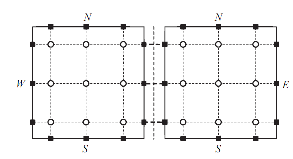
其中, 右上标"$\delta$"代表近似解, "D"表示是单元上的局部解, $\hat{u}^{\delta D}_{i, j}$是求解点$(\xi_{i}, \eta_{j})$处的近似解, $l_{i}$和$l_{j}$是相对应的拉格朗日插值多项式. $\hat{u}^{\delta D}(\xi, \eta, t)$在单元内部是连续的, 但在相邻单元之间是间断的. 图2中给出了$p=2$时在四边形单元上求解点和后续用于通量修正的边界面通量点的分布.

图2

新窗口打开|下载原图ZIP|生成PPT
图2两个四边形单元上求解点(圆圈)和通量点(方块)的分布($p=2$)

Fig.2Arrangement of solution points (circles) and flux points (squares) on a pair of quadrilateral elements ($p=2$)



在计算散度项之前, 首先进行通量项的构造和计算. 参照方程(9)中近似解$\hat{u}^{\delta D}$的构造, 同样可以获取局部通量$\hat{{ f }}^{\delta D}$. 但由于$\hat{{ f }}^{\delta D}$仅在单元内部连续, 而在单元之间并不连续. 为了满足格式守恒性的要求, FR通过增加修正项的方式构造在单元界面处连续的通量. 因此, 连续的全局通量$\hat{{ f }}^{\delta}=(\hat{f}^{\delta}, \hat{g}^{\delta})$由单元内的局部通量$\hat{{ f }}^{\delta D}$和修正通量$\hat{{ f }}^{\delta C}$构成

(10)$\hat{{ f }}^{\delta} = \hat{{ f }}^{\delta D} + \hat{{ f }}^{\delta C}$
上式中, 局部通量$\hat{{ f }}^{\delta D}=(\hat{f}^{\delta D}, \hat{g}^{\delta D})$通过$p$阶的插值多项式进行近似

(11)$\hat{{ f }}^{\delta D}(\xi, \eta, t) = \sum_{i=1}^{p+1} \sum_{j=1}^{p+1}\hat{{ f }}^{\delta D}_{i, j}l_{i}(\xi)l_{j}(\eta)$
其中, $\hat{{ f }}^{\delta D}_{i, j}=(f^{\delta D}_{i, j}, g^{\delta D}_{i, j})$ 是求解点$(\xi_{i}, \eta_{j})$处的通量值, 其值由$\hat{u}^{\delta D}_{i, j}$直接计算得到. 进而可得局部通量$\hat{{ f }}^{\delta D}$的散度为

(12)$\nabla_{\xi \eta} \cdot \hat{{ f }}^{\delta D} = \sum_{i=1}^{p+1} \sum_{j=1}^{p+1} \hat{f}^{\delta D}_{i, j} l_{i}'(\xi) l_{j}(\eta) + \\ \sum_{i=1}^{p+1} \sum_{j=1}^{p+1} \hat{g}^{\delta D}_{i, j} l_{i}(\xi) l_{j}\prime(\eta)$
同时, 求解点$(\xi_{i}, \eta_{i})$上修正通量项$\hat{{ f }}^{\delta C}$的散度$\nabla_{\xi \eta} \cdot \hat{{ f }}^{\delta C}$如下

(13)$\begin{align} \nabla_{\xi \eta} \cdot \hat{{ f }}^{\delta C} = \dfrac{\partial \hat{f}^{\delta C}(\xi_{i}, \eta_{j})}{\partial \xi} + \dfrac{\partial \hat{g}^{\delta C}(\xi_{i}, \eta_{j})}{\partial \eta} = \\ \left[(\hat{{ f }} \cdot \hat{n})^{\delta I}_W-\hat{f}^{\delta D}_W \right] \dfrac{d h_W}{d \xi} + \left[(\hat{{ f }} \cdot \hat{n})^{\delta I}_E-\hat{f}^{\delta D}_E \right] \dfrac{d h_E}{d \xi}+ \\ \left[(\hat{{ f }} \cdot \hat{n})^{\delta I}_S-\hat{f}^{\delta D}_S \right] \dfrac{d h_S}{d \eta} + \left[(\hat{{ f }} \cdot \hat{n})^{\delta I}_N-\hat{f}^{\delta D}_N \right] \dfrac{d h_N}{d \eta} \end{align}$
上式中, $\hat{f}^{\delta D}_W$, $\hat{f}^{\delta D}_E$, $\hat{g}^{\delta D}_S$和$\hat{g}^{\delta D}_N$分别是四边形单元4条边上通量点处的不连续通量值, 它们的值由单元局部近似解$\hat{{ f }}^{\delta D}_{i, j}$外插得到. $(\hat{{ f }} \cdot \hat{n})^{\delta I}_W$, $(\hat{{ f }} \cdot \hat{n})^{\delta I}_E$, $(\hat{{ f }} \cdot \hat{n})^{\delta I}_S$ 和 $(\hat{{ f }} \cdot \hat{n})^{\delta I}_N$分别为界面处连续的法向数值通量, 它们的值需通过黎曼求解器(Riemmann Solvers), 例如常见的Roe^[33], Rusanov^[34]等来计算, 在本文中使用的是Rusanov格式. $h_E$, $h_S$, $h_W$和$h_N$是$p+1$阶修正多项式. 当修正多项式为Radau多项式时, 可证明对于线性问题而言, 此时的FR格式等价于节点型的DG格式^{[11, 20]}.

综上, 经过FR格式空间离散之后的半离散方程为

(14)$\dfrac{d \hat{u}^{\delta D}}{dt} =- \nabla_{\xi \eta} \cdot \hat{{ f }}^{\delta}= - \left[ \nabla_{\xi \eta} \cdot \hat{{ f }}^{\delta D} + \nabla_{\xi \eta} \cdot \hat{{ f }}^{\delta C} \right]$
上述常微分方程组可进一步通过显式或隐式的时间推进方法进行求解.

3 隐式时间推进方法

二维欧拉方程经过空间离散之后得到的半离散方程可进一步写作如下形式

(15)$\dfrac{d { U}(t)}{d t} = { R}({ U})$
在上式中

${ U}(t)=\left[\overbrace{{ U}_1^1, {{ U}_1^2, \cdots , { U}_1^N}}^{{ U}_{1}(t)}, \cdots , \overbrace{{ U}_M^1, {{ U}_M^2, \cdots , { U}_M^N}}^{{ U}_{M}(t)} \right]^T$

为$M \times N \times 4$维度的全局解向量, 其中, $M$和$N$分别代表网格单元总数以及每个单元内求解点的个数, ${ U}_{M}(t)$为第$M$个单元上的局部解, ${ U}_{M}^{N}$是第$M$个单元第$N$个求解点上包含守恒变量的解向量.

${ R}({ U})=[\overbrace{{ R}_1^1({ U}), { R}_1^2({ U}), \cdots , { R}_1^N({ U})}^{{ R}_{1}({ U})}, \cdots , \\ \overbrace{ { R}_M^1({ U}), { R}_M^2({ U}), \cdots , { R}_M^N({ U})}^{{ R}_{M}({ U})} ]^T$

代表右端残差项, ${ R}_{M}({ U})$是第$M$个单元上的局部残差, ${ R}_{M}^{N}({ U})$为第$M$个单元第$N$点上残差.

由于本文计算的是定常流动, 无需考虑时间精度, 因此时间项的离散使用一阶向后隐式差分格式. 方程(15)经过该方法离散后可得

(16)${ U}^{n+1}-{ U}^n=\Delta { T}^n { R}({ U}^{n+1})$
式中, ${ U}^{n}={ U}(t^{n})$和${ U}^{n+1}={ U}(t^{n+1})$分别为$t^{n}$和$t^{n+1}$时刻的解. $\Delta { T}^n$为一个包括时间步长的对角矩阵, 其与${ U}^{n}$具有相同的维数, 其具体形式为

(17)$\Delta { T}^n=\text{diag}\left\{\overbrace{\Delta {t}_1^{1, n}, \Delta {t}_1^{2, n}, \cdots , \Delta {t}_1^{N, n}}^{\Delta { T}_1^{n}}, \cdots , \overbrace{\Delta {t}_M^{1, n}, \Delta {t}_M^{2, n}, \cdots , \Delta {t}_{M}^{N, n}}^{\Delta { T}_M^{n}} \right\}$
式中, $\Delta {t}_{M}^{N, n}$表示第$n$次迭代时在第$M$个单元第$N$个求解点处的时间步长. 对于二维欧拉方程, $\Delta {t}_{M}^{N, n}$是一个$4 \times 4$的对角阵, 其对角元素的值均为该点处由CFL条件计算的时间步长.

由于方程(16)中的${ R}({ U}^{n+1})$是非线性的, 通过泰勒展开对其线性化, 则有

(18)${ R}({ U}^{n+1}) \approx { R}({ U}^{n}) + \left. \dfrac{\partial { R}}{\partial { U}} \right |_{{ U}^{n}}({ U}^{n+1}-{ U}^n)$
上式中, ${\partial { R}}/{\partial { U}} |_{{ U}^{n}}$为全局雅可比矩阵. 将方程(18)代入方程(16)并整理得

(19)$\left[ (\Delta { T}^n)^{-1} - \left. \dfrac{\partial { R}}{\partial { U}} \right |_{{ U}^{n}} \right] ({ U}^{n+1}-{ U}^n) = { R}({ U}^{n})$
上式中, $t^{n+1}$时的解${ U}^{n+1}$需要先求解线性方程组才能获取.

3.1 块雅可比迭代

线性方程组的求解可分为直接法和迭代法. 当网格规模较大时, 使用直接法求解效率低下且内存占用较大. 因此本文通过迭代法求解方程(19), 所用的迭代方法为雅可比迭代.

首先对方程(19)左端的矩阵进行分解. 令${ A} = \left[ (\Delta { T}^n)^{-1} - {\partial { R}}/{\partial { U}} |_{{ U}^{n}} \right]$. 则${ A} = { D} - { N}$可看作是由分块对角矩阵${ D}$和剩余非对角部分${ N}$组成. 其中, 分块对角矩阵$ D$为

(20)${ D} = \text{diag}\{(\Delta { T}_1^{n})^{-1} - { J}^{n}_{1}, \ \ (\Delta { T}_2^{n})^{-1} - { J}^{n}_{2}, \cdots , \\ (\Delta { T}_M^{n})^{-1} - { J}^{n}_{M}\}$
上式中, ${ J}^{n}_{M}$是第$M$个单元上的局部雅可比矩阵, 其维度为$4 N \times 4 N$.

第$i$个单元上的单元雅克比矩阵${ J}_{i}^{n}$可进一步展开为以下矩阵形式

(21)$ { J}^{n}_{i}= \left[ \begin{array}{ccc} \left. \dfrac{\partial { R}^1_i({ U})}{\partial { U}^1_i} \right |_{{ U}^{n}} & \cdots & \left. \dfrac{\partial { R}^1_i({ U})}{\partial { U}^N_i} \right |_{{ U}^{n}} \\ \vdots & \ddots & \vdots \\ \left. \dfrac{\partial { R}^N_i({ U})}{\partial { U}^1_i} \right |_{{ U}^{n}} & \cdots & \left. \dfrac{\partial { R}^N_i({ U})}{\partial { U}^N_i} \right |_{{ U}^{n}} \\ \end{array} \right], i=1, 2, \cdots , M$
与此同时, $N$的矩阵形式是

(22)$ N=\left( \begin{array}{ccccccc} & & \cdots & \left. \dfrac{\partial { R}_1^1}{\partial { U}_M^1} \right |_{{ U}^{n}} & \cdots & \left. \dfrac{\partial { R}_1^1}{\partial { U}_M^N} \right |_{{ U}^{n}} \\ & 0 & \cdots & \vdots & \ddots & \vdots \\ & & & \cdots & \left. \dfrac{\partial { R}_1^N}{\partial { U}_M^1} \right |_{{ U}^{n}} & \cdots & \left. \dfrac{\partial { R}_1^N}{\partial { U}_M^N}\right |_{{ U}^{n}}\\ \vdots & \vdots & \vdots & \ddots & \vdots & \vdots & \vdots \\ \left. \dfrac{\partial { R}_M^1}{\partial { U}_1^1} \right |_{{ U}^{n}}& \cdots & \left. \dfrac{\partial { R}_M^1}{\partial { U}_1^N} \right |_{{ U}^{n}} & \cdots & & & \\ \vdots & \ddots & \vdots & \cdots & & 0 & \\ \left. \dfrac{\partial { R}_M^N}{\partial { U}_1^1}\right |_{{ U}^{n}} & \cdots & \left. \dfrac{\partial { R}_M^N}{\partial { U}_1^N}\right |_{{ U}^{n}} & \cdots & & & \\ \end{array} \right)$
式中的${ N}$为一稀疏矩阵. 经过上述分解之后, 对全局线性方程组(19)进行迭代求解, 可得

(23)${ D} ({ U}^{k+1}-{ U}^n)= { N} ({ U}^k-{ U}^n)+ { R} ({ U}^n), k=0, 1, 2, \cdots$
在上式中, $k$为雅可比迭代指标. 当$k \rightarrow \infty$时, 雅可比迭代解${ U}^{k+1}$趋近于下一个时刻的解${ U}^{n+1}$. 对于定常问题的计算, $k$只需要设置为有限的值, 当$n \rightarrow \infty$, ${ U}^{k+1}$和${ U}^{n}$最终都将趋向于所求的定常解.

为了避免非对角部分${ N}$的计算. 对方程(23)两侧同时减去${ D} ({ U}^k-{ U}^n)$, 则有

(24)${ D} ({ U}^{k+1}-{ U}^n-{ U}^k+{ U}^n)= ({ N}-{ D}) ({ U}^k-{ U}^n)+ { R} ({ U}^n)$
上式经进一步整理后可得

(25)${ D} ({ U}^{k+1} -{ U}^k)=- \left[ (\Delta { T}^n)^{-1} - \left. \dfrac{\partial { R}}{\partial { U}} \right |_{{ U}^{n}} \right] ({ U}^k-{ U}^n)+ { R} ({ U}^n)$
和方程(18)类似, 将${ R} ({ U}^k)$在${ R} ({ U}^n)$处进行泰勒展开

(26)${ R} ({ U}^k) \approx { R} ({ U}^n) + \left. \dfrac{\partial { R}}{\partial { U}} \right |_{{ U}^{n}} ({ U}^k-{ U}^n)$
上式可进一步写成

(27)${ R} ({ U}^n) \approx { R} ({ U}^k) - \left. \dfrac{\partial { R}}{\partial { U}} \right |_{{ U}^{n}} ({ U}^k-{ U}^n)$
将方程(27)代入到方程(25)中消去全局矩阵相关的一项${\partial { R}}/{\partial { U}} |_{{ U}^{n}} ({ U}^k-{ U}^n)$, 并最终整理可得

(28)${ D} ({ U}^{k+1} -{ U}^k) = { R} ({ U}^k)- (\Delta { T}^n)^{-1} ({ U}^k-{ U}^n)$
式中, ${ D}=\text{diag} \{{ D}_1, { D}_2, \cdots , { D}_{M}\}$.

方程(28)和方程(19)相比, 它的左端矩阵${ D}$是一个分块对角矩阵, 这使得求解全局线性方程组(19)的问题解耦为求解一系列局部单元上的小型线性方程组.

值得注意的是, 全局矩阵${ A}$的分解方式并不唯一, 如将其分解为分块上三角矩阵${ U}$和分块下三角矩阵${ L}$, 即为Gauss-Seidel迭代法. 此时需要求解的方程的左端矩阵为分块下三角矩阵${ L}$. 由于此时${ U}^{k+1}$存在数据依赖问题, 无法同时更新, 为了并行地求解该方程, 需要使用图着色技术, 所得方法即为更复杂的MCGS法^[26].

3.2 局部线性方程组的求解

方程(28)可进一步写成一系列局部单元线性方程组. 对于第$i$ ($1\leqslant i \leqslant M$)个单元, 则有

(29)${ D}_i ({ U}^{k+1}_i -{ U}^k_i) = \left[ (\Delta { T}^n_i)^{-1} - { J}^n_i \right] ({ U}^{k+1}_i -{ U}^k_i)- { R}_{i} ({ U}^k)- (\Delta { T}^n_i)^{-1} ({ U}^k_i-{ U}^n_i)$
上式中, $i$为单元指标, $n$是时间迭代指标, $k$为雅可比迭代指标. ${ J}^n_i$为第$i$个单元对应的单元雅可比矩阵, 在下一小节中将讨论其具体计算方法. 以上获取的$M$个局部线性方程组(29), 其左端矩阵规模较小, 在程序中通过调用cuBLAS函数库使用LU分解法实现同步求解.

3.3 单元雅可比矩阵${ J}^n_i$的计算

方程(29)中, ${ J}^n_i$的计算对隐式方法的精度、效率以及稳定性有较大的影响. 雅可比矩阵常见的计算方式有解析法^[26]、有限差分近似^[35]和自动微分^[36]等方法.

本文中所用是解析法与自动微分相结合的方法. 由式(13)可知, 第$i$个单元上, FR格式离散后的残差${ R}_i$是不连续通量的散度${ R}_i^D$和修正通量${ R}_i^C$的散度之和. 则单元雅可比矩阵为

${ J}^{n}_{i}=\dfrac{\partial { R}^C_i}{\partial { U}_i} + \dfrac{\partial { R}^D_i}{\partial { U}_i}$

其中, ${\partial { R}^D_i}/{\partial { U}_i}$只与当前单元的解有关, 借鉴文献[26, 37]中的做法, 这部分的雅可比矩阵可通过解析的方法精确获取. 对于二维欧拉方程, 其形式为

(30)$\dfrac{\partial { R}^D_i}{\partial { U}_i} = - \left( { D}_{\xi} \dfrac{\partial \hat{{ F}}^{\delta D}_i}{\partial { U}_{i}} + { D}_{\eta} \dfrac{\partial \hat{{ G}}^{\delta D}_i }{\partial { U}_{i}} \right)$
式中, ${ D}_{\xi}$ 和 ${ D}_{\eta}$分别为$\xi$和$\eta$方向的插值多项式微分算子, ${\partial \hat{{ F}}^{\delta D}_i}/{\partial { U}_{i}}$和${\partial \hat{{ G}}^{\delta D}_i}/{\partial { U}_{i}}$为计算域$(\xi, \eta)$上通量项$\hat{{ F}}^{\delta D}_i$和$\hat{{ G}}^{\delta D}_i$关于${ U}_{i}$的导数, 根据式(8)可知

(31)$\dfrac{\partial \hat{{ F}}^{\delta D}_i}{\partial { U}_{i}} = \dfrac{\partial y}{\partial \eta}\dfrac{\partial { F}^{\delta D}_i}{\partial { U}_{i}} -\dfrac{\partial x}{\partial \eta}\dfrac{\partial { G}^{\delta D}_i}{\partial { U}_{i}}$
(32)$\dfrac{\partial \hat{{ G}}^{\delta D}_i}{\partial { U}_{i}} = \dfrac{\partial x}{\partial \xi}\dfrac{\partial { G}^{\delta D}_i}{\partial { U}_{i}} - \dfrac{\partial y}{\partial \xi}\dfrac{\partial { F}^{\delta D}_i}{\partial { U}_{i}}$
其中, ${\partial { F}^{\delta D}_i}/{\partial { U}_{i}}$和${\partial { G}^{\delta D}_i}/{\partial { U}_{i}}$分别是物理域$(x, y)$上${ F}^{\delta D}_i$和${ G}^{\delta D}_i$关于${ U}_{i}$的导数. 对于二维欧拉方程, 这两者都是已知的, 它们的具体形式在附录中给出.

对于修正项残差${ R}_i^C$而言, 其中计算单元交接面法向数值通量的黎曼求解器需要用到相邻单元的解. 当黎曼求解器使用较为简单的Rusanov格式时, 其精确形式能被推导出来^[26]. 但如果是Roe等复杂格式, 就很难获取其精确的解析形式. 本文中对于${\partial { R}^C_i}/{\partial { U}_i}$的计算是通过调用自动微分函数库Sacado^[38]实现的. 这种解析法结合自动微分技术计算单元雅克比矩阵的方式虽然相对于纯解析方式损失了部分精度, 但无疑其适用范围更加广泛.

4 数值实验

本节中以二维Bump流动和NACA0012翼型无黏绕流两个算例来展示隐式方法的精度和效率. 为了进行计算效率的对比研究, 所有算例均同时使用显式和隐式两类方法进行. 显式方法为具有TVD性质的三级Runge-Kutta (TVD RK3)方法^[21], 同时使用局部时间步长和多重网格($p$ multi-grid)方法加速其收敛. 隐式方法为本文中所提出的块雅可比迭代的方法. 隐式方法的时间步长$\Delta { T}^{n}$由CFL数决定, CFL数初始值为2, 并随迭代步数指数增长, 最大值为$10^4$.

所有算例均使用高阶并行通量重构软件HAFR (heterogeneous architecture flux reconstruction)在型号为英伟达GeForce RTX 2080ti的单个GPU卡上计算. 为了保证FR方法在边界的精度不至于下降, 算例中用到的网格是由开源网格生成软件Gmsh生成的二阶曲边网格. 计算的收敛性通过密度残差的$L^2$范数判断, 当其下降到$10^{-14}$以下或平稳而不再下降时便认为计算已稳态收敛并终止.

4.1 无黏亚声速Bump算例

本算例是international workshop on high-order CFD methods^[39]给定的一个二维无黏验证算例. 该问题的物理域为$[-1.5, 1.5] \times [0, 0.8]$, 底边的几何描述为$y=0.062 5e^{-25x^2}$. 左侧为亚声速入口边界条件(给定入口总压和总温), 右侧出口为出口边界条件(给定静压), 上下边界均为滑移壁面边界条件. 来流的马赫数$Ma=0.5$且攻角为零度. 尽管该流动的精确解未知, 但由于流动为亚声速无黏流动且流场光滑, 因此可通过熵来衡量解的精度, 流场中熵的计算公式如下

(33)$||Es||_{L^{2}(\varOmega )}=\sqrt{\dfrac{ \int_{\varOmega }(\dfrac{p}{p_{\infty}}(\dfrac{\rho _{\infty}}{\rho } )^{\gamma} - 1 )^2d V}{\int_{\varOmega } d V}}$
式中的积分在HAFR程序中通过10阶高斯积分法进行计算.

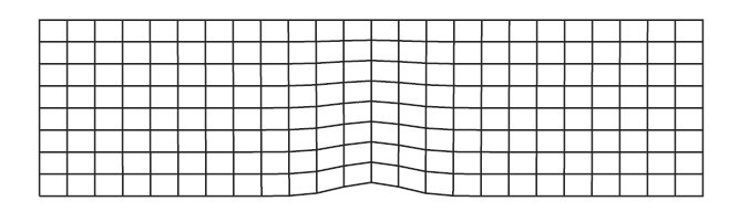
计算中所使用的网格由粗到细(即$h$-refinement)为：R1($12\times4$), R2($24\times8$), R3($48\times16$)和R4($96\times32$), 图3是R2网格的示例. 对于同一网格, 同时还将使用$p=2, 3, 4$阶的插值多项式(即$p$-refinement)进行计算.

图3

新窗口打开|下载原图ZIP|生成PPT
图3本算例中所用的$24\times8$的四边形网格

Fig.3Quadrangular mesh ($24\times8$) used in the case



首先从数值精度的角度分析计算结果. 表1为HAFR程序使用块雅可比迭代隐式方法在四组网格上, 插值多项式为$p=2, 3, 4$阶时的熵以及数值精度. 从表中可知, 对任意一阶插值多项式阶数而言, 网格加密的过程中熵也随之降低. 同时, 给定某组网格, 提高插值多项式的阶数也同样会导致熵的降低. 正如图4所示, 在R2网格上使用$p=3$和$p=4$阶插值多项式得到的下壁面马赫数等值线相比$p=2$的更为光滑. 此外还观察到, 对于$p=2, 3, 4$阶插值多项式, 在4组网格上获取的数值精度, 都近似达到$p+1$阶这一理论值, 这也验证了HAFR的计算精度.

Table 1
表1
表1在四组网格上, 使用$p=2$, 3, 4阶多项式时的熵和数值精度
Table 1Entropies and numerical orders on four different grids with $p=2$, 3, 4 polynomial orders

新窗口打开|下载CSV

图4

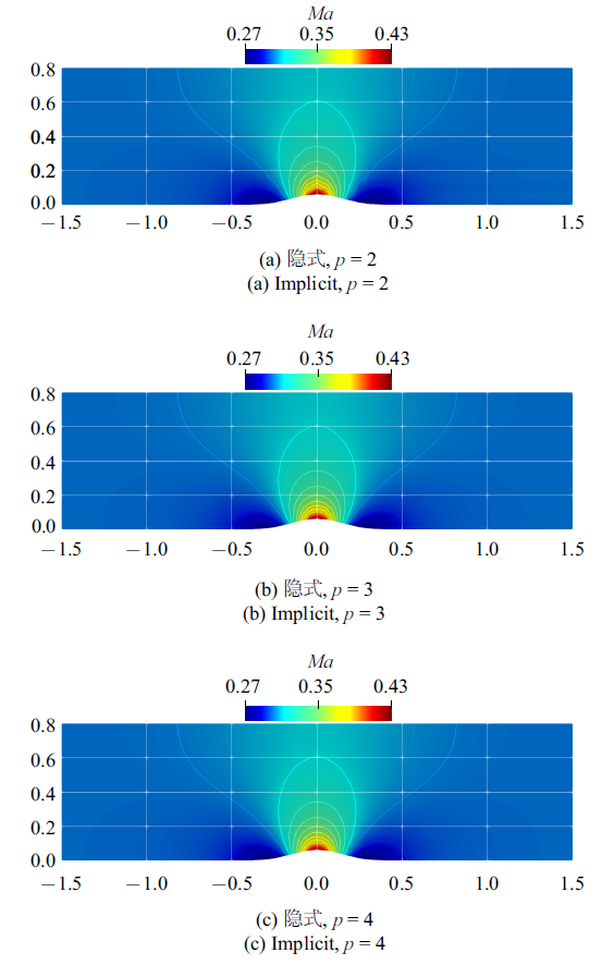新窗口打开|下载原图ZIP|生成PPT
图4在$24\times8$的网格上使用 $p = 2$, 3, 4 阶插值多项式计算所得的马赫数云图

Fig.4Mach number contours calculated on the $24\times8$ mesh with $p = 2$, 3, 4 polynomial orders



下面从计算效率的角度进行分析. 图5是HAFR程序使用显式和隐式两种方法在4组网格上、插值多项式为$p=2, 3, 4$阶时密度残差随迭代次数的收敛情况.

图5

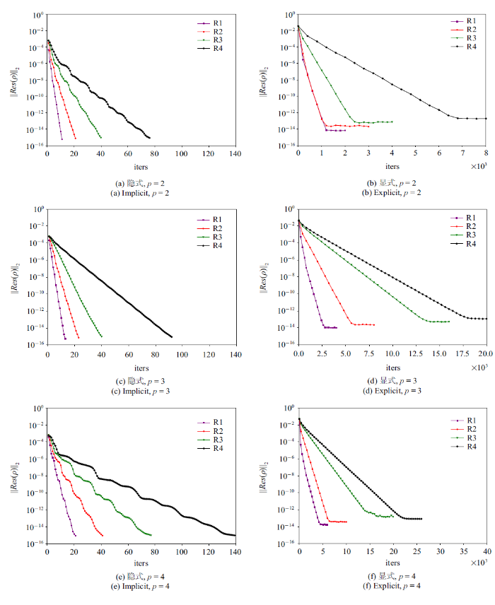新窗口打开|下载原图ZIP|生成PPT
图5在四组网格上, 插值多项式为 $p=2$, 3, 4阶时, 使用隐式和显式方法所得到的密度残差$||Res(\rho )||_{2}$随迭代次数的变化

Fig.5Density residual $||Res(\rho )||_{2}$ versus the iteration numbers for the explicit and implicit time-marching schemes on four different grids with $p=2$, 3, 4 polynomial orders



在图5中, 左右两列子图分别为使用块雅可比迭代隐式和TVD RK3显式时间方法的计算结果. 从迭代次数来看, 对同一阶插值多项式, 显式方法和隐式方法收敛所需的迭代次数都随着网格的加密而增大. 对于同一网格, 使用更高阶的插值多项式都会导致迭代次数的增多. 但同时发现, 隐式方法的迭代次数随自由度(degree of freedom, DoF)增幅较小, 并且对于同一网格或同一阶插值多项式, 隐式方法所需的迭代次数要远远小于显式方法. 例如, 在R1网格上, 隐式方法收敛的的迭代次数均在80步以内, 而显式方法最快也需要1000步左右才能收敛.

在密度残差收敛方面, 使用隐式方法的计算的密度残差均能收敛到$10^{-14}$这一量级. 但显式方法的收敛性随着自由度的增大变差, 其值下降到某个量级后将无法下降, 例如使用$p=2$阶插值多项式时, 在R1网格上的密度残差能够收敛$10^{-14}$量级, 但在R4网格上仅能下降到$10^{-13}$这一量级.

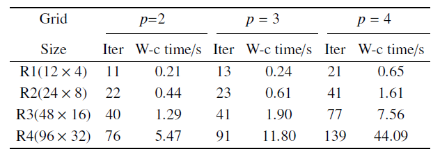
在GPU计算时间方面, 表2为HAFR程序采用块雅可比迭代隐式方法在4组网格上, 使用$p=2, 3, 4$阶插值多项式计算收敛所用的迭代次数和GPU墙钟时间. 从表2可知, 隐式方法计算收敛所用时间随着自由度的增大而增大.

Table 2
表2
表2在四组网格上, 插值多项式为 $p = 2$, 3, 4阶时, 使用隐式时间方法时的迭代次数和墙钟时间
Table 2Iteration numbers and wall-clock times for the implicit time-marching scheme on four different grids with $p = 2$, 3, 4 polynomial orders

新窗口打开|下载CSV

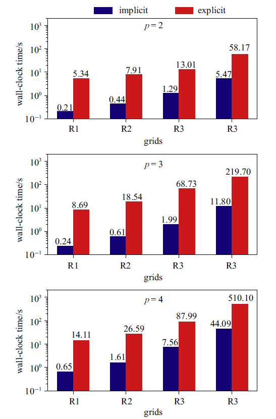
图6是HAFR程序分别使用块雅可比隐式和TVD RK3显式时间方法, 在不同网格上, 使用$p=2, 3, 4$阶插值多项式时所用的墙钟时间对比. 从图6中可看到, 对每一组计算, 隐式方法收敛所用的时间明显小于显式方法. 在所有算例中, 隐式方法相比显式至少有一个量级的加速效果.

图6

新窗口打开|下载原图ZIP|生成PPT
图6在四组网格上, 插值多项式为 $p = 2$, 3, 4阶时, 使用隐式和显式方法所用的计算时间

Fig.6Wall-clock times for the explicit and implicit time-marching schemes on four different grids with $p=2$, 3, 4 polynomial orders

4.2 NACA0012翼型无黏绕流

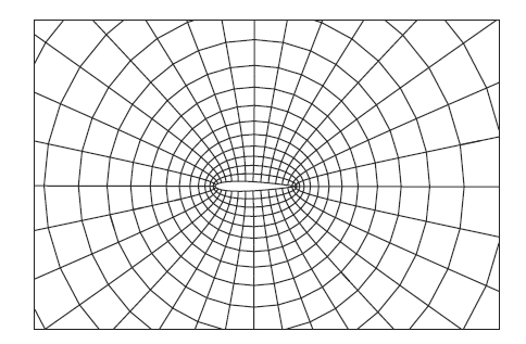
在上一个Bump算例中所使用的网格较为均匀, 为了进一步考察在非均匀网格条件下块雅可比迭代隐式方法的计算效率, 下面对NACA0012翼型无黏绕流进行数值模拟. 在此算例中, 自由来流的马赫数为0.5且攻角为零度. NACA0012翼型表面为滑移壁面条件, 远场为特征边界条件, 远场与翼型的距离大约为100个弦长.

计算中用到的网格为Gmsh生成的O型网格, 网格分为3组：R1($32\times32$), R2($44\times64$)和R3($128\times128$). 图7为R1($32\times32$)网格的示意图. 对于同一网格, 还将分别使用$p=2, 3, 4$阶的插值多项式(即$p$-refinement)进行计算.

图7

新窗口打开|下载原图ZIP|生成PPT
图7本算例中所用的$32\times32$的O型四边形网格

Fig.7O-type quadrangular mesh ($32\times32$) used in this case



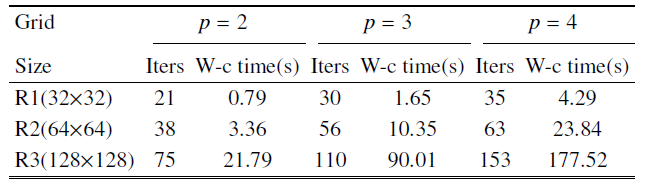
下面对NACA0012数值模拟结果进行分析. 表3为HAFR程序采用块雅可比迭代隐式方法在三组网格上, 使用$p=2, 3, 4$阶插值多项式计算收敛所用的迭代次数和GPU墙钟时间. 和上个算例中类似, 可观察到无论是网格加密还是提高插值多项式阶数, 这两种增大自由度的方式都会导致迭代次数和GPU计算时间的增多.

Table 3
表3
表3在三组网格上, 插值多项式为 $p = 2$, 3, 4阶时, 使用隐式时间方法时的迭代次数和墙钟时间
Table 3Iteration numbers and wall-clock times for the implicit time-marching schemes on three different grids with $p=2$, 3, 4 polynomial orders

新窗口打开|下载CSV

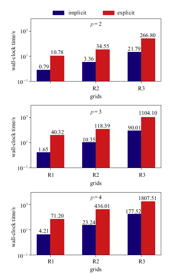
图8是HAFR程序分别使用隐式和显式时间方法, 在不同网格上, 使用插值多项式为$p=2, 3, 4$时所用的墙钟时间对比. 从图8中可知, 对于每一组计算, 使用块雅可比迭代隐式方法收敛所用的时间相比TVD RK3显式方法至少有一个量级的加速效果.

图8

新窗口打开|下载原图ZIP|生成PPT
图8在三组网格上, 插值多项式为 $p = 2$, 3, 4阶时, 使用隐式和显式方法所用的墙钟时间

Fig.8Wall-clock times for the explicit and implicit time-marching schemes on three different grids with $p=2$, 3, 4 polynomial orders



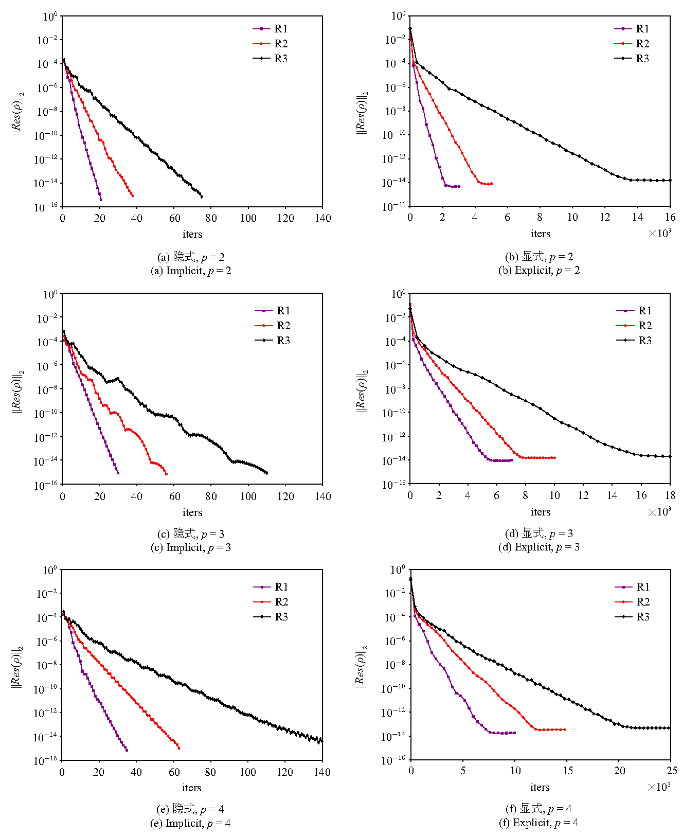
图9为HAFR程序使用显式和隐式两种方法在三组网格上、插值多项式为$p=2, 3, 4$阶时密度残差随迭代次数的收敛情况. 在图9中, 左右两列子图分别为使用块雅可比迭代隐式和TVD RK3显式时间方法的结果. 从迭代次数来看, 对同一阶插值多项式, 显式方法和隐式方法收敛所需的迭代次数都随着网格的加密而增大. 对于同一网格, 使用更高阶的插值多项式会导致迭代次数的增多. 但同时, 相比显式方法, 隐式方法的迭代次数随自由度增幅较小, 并且对于同一网格或同一阶插值多项式, 隐式方法所需的迭代次数要远远小于显式方法.

图9

新窗口打开|下载原图ZIP|生成PPT
图9在三组网格上, 插值多项式为 $p = 2$, 3, 4阶时, 使用隐式和显式方法所得到的密度残差$||Res(\rho )||_{2}$随迭代次数的变化

Fig.9Density residual $||Res(\rho )||_{2}$ versus the iteration numbers for the explicit and implicit time-marching schemes on three different grids with $p=2$, 3, 4 polynomial orders



在密度残差收敛方面, 在3组网格计算中, 使用块雅可比迭代隐式方法计算的密度残差均能收敛到$10^{-14}$这一量级. 但TVD RK3显式时间方法的收敛性随着自由度的增大变差, 其值下降到某个量级后将无法下降. 因此从残差收敛角度, 基于块雅可比迭代的隐式方法要优于TVD RK3显式方法.

综上, 随着自由度的增大, 显式和隐式方法收敛所需的迭代次数都会增多. 但对于同一网格或同一阶插值多项式, 隐式方法所需的迭代次数和计算时间要明显小于显式方法, 且隐式方法的残差下降幅度要比显式方法更大.

5 结论

为了提高FR方法的求解效率, 本文提出一种基于雅可比块迭代的高阶FR格式求解定常二维欧拉方程的单GPU隐式时间推进方法. 通过雅可比块迭代的方式, 克服了影响求解并行性的相邻单元依赖, 使得只需存储和计算对角块矩阵. 最终将求解全局线性方程组转化为求解一系列局部单元线性方程组. 这些局部的线性方程组在GPU上又可利用LU分解法并行求解.

文中通过二维无黏Bump流动和NACA0012无黏绕流两个算例表明: 随着自由度的增大, 块雅可比迭代隐式方法收敛所需的迭代次数和计算时间都会增多. 但对于同一网格或同一阶插值多项式, 该隐式方法所需的迭代次数要明显小于TVD RK3显式方法, 且此隐式方法的残差下降幅度要比TVD RK3显式方法更大. 在计算时间方面, 对于文中的每一组计算, 雅可比块迭代隐式方法收敛所用的GPU计算时间明显小于TVD RK3显式方法, 且计算效率至少有一个量级的提高.

附录

二维欧拉方程的雅克比矩阵为

(A1)$\dfrac{\partial { F}}{\partial { U}}= \left( \begin{array}{c@{\ \ \ }c@{\ \ \ }c@{\ \ \ }c} 0 & 1 & 0 & 0 \\ \dfrac{1}{2} \left((\gamma -3) u^2+(\gamma -1) v^2\right) & (3-\gamma ) u & (1-\gamma ) v & \gamma -1 \\ -u v & v & u & 0 \\ (\gamma -1) u \left(u^2+v^2\right)-\dfrac{\gamma e u}{\rho } & (\gamma -1) \left(3 u^2+v^2\right)+\dfrac{\gamma e}{\rho } & (1-\gamma ) u v & \gamma u \\ \end{array} \right)$
以及

(A2)$\dfrac{\partial { G}}{\partial { U}}= \left( \begin{array}{c@{\ \ \ }c@{\ \ \ }c@{\ \ \ }c} 0 & 0 & 1 & 0 \\ -u v & v & u & 0 \\ \dfrac{1}{2} \left((\gamma -1) u^2+(\gamma -3) v^2\right) & (1-\gamma ) v & (3-\gamma ) v & \gamma -1 \\ (\gamma -1) v \left(u^2+v^2\right)-\dfrac{\gamma e u}{\rho } & (1-\gamma ) u v & \dfrac{\gamma e}{\rho }+(\gamma -1) \left(u^2+3 v^2\right) & \gamma v \\ \end{array} \right)$

参考文献 View Option 原文顺序
文献年度倒序
文中引用次数倒序
被引期刊影响因子

[1] Slotnick J, Khodadoust A, Alonso J, et al. CFD Vision 2030 Study: A path to revolutionary computational aerosciences
NASA/CR-2014-218178, Washington: NASA, 2014
[本文引用: 1]

[2] 阎超, 屈峰, 赵雅甜 等. 航空航天CFD物理模型和计算方法的述评与挑战
空气动力学学报, 2020, 38(5): 829-857
[本文引用: 1]

(Yan Chao, Qu Feng, Zhao Yatian, et al. Review of development and challenges for physical modeling and numerical scheme of CFD in aeronautics and astronautics
Chinese Journal of Theoretical and Applied Mechanics, 2020, 38(5): 829-857 (in Chinese))
[本文引用: 1]

[3] Jiang GS, Shu CW. Efficient implementation of weighted ENO schemes
Journal of Computational Physics, 1996, 126(1): 202-228
DOIURL [本文引用: 1]

[4] Deng XG, Zhang HX. Developing high-order weighted compact nonlinear schemes
Journal of Computational Physics, 2000, 165(1): 22-44
DOIURL [本文引用: 1]

[5] Tsoutsanis P, Titarev A, Drikakis D. WENO schemes on arbitrary mixed-element unstructured meshes in three space dimensions
Journal of Computational Physics, 2011, 230(4): 1585-1601
DOIURL [本文引用: 1]

[6] Wang Q, Ren YX, Pan J, et al. Compact high order finite volume method on unstructured grids III: Variational reconstruction
Journal of Computational Physics, 2017, 337: 1-26
[本文引用: 1]

[7] Cockburn B, Lin SY, Shu CW. TVB Runge-Kutta local projection discontinuous Galerkin finite element method for conservation laws III: One-dimensional systems
Journal of Computational Physics, 1989, 84(1): 90-113
DOIURL [本文引用: 1]

[8] Cockburn B, Shu CW. Runge-Kutta discontinuous Galerkin methods for convection-dominated problems
Journal of Scientific Computing, 2001, 16(3): 173-261
DOIURL [本文引用: 1]

[9] Wang ZJ. Spectral (finite) volume method for conservation laws on unstructured grids: Basic formulation
Journal of Computational Physics, 2002, 178(1): 210-251
DOIURL [本文引用: 1]

[10] Liu Y, Vinokur M, Wang ZJ. Spectral difference method for unstructured grids I: Basic formulation
Journal of Computational Physics, 2006, 216(2): 780-801
DOIURL [本文引用: 1]

[11] Huynh HT. A flux reconstruction approach to high-order schemes including discontinuous Galerkin methods//18th AIAA Computational Fluid Dynamics Conference, 2007
[本文引用: 2]

[12] Huynh HT. A reconstruction approach to high-order schemnes including discontinuous Galerkin for diffusion//47th AIAA Aerospace Sciences Meeting Including the New Horizons Forum and Aerospace Exposition, 2009
[本文引用: 1]

[13] Wang ZJ, Gao H. A unifying lifting collocation penalty formulation including the discontinuous Galerkin, spectral volume/difference methods for conservation laws on mixed grids
Journal of Computational Physics, 2009, 228(21): 8161-8186
DOIURL [本文引用: 1]

[14] Huynh HT, Wang ZJ, Vincent P. High-order methods for computational fluid dynamics: A brief review of compact differential formulations on unstructured grids
Computers & Fluids, 2014, 98: 209-220
DOIURL [本文引用: 1]

[15] Vincent P, Castonguay P, Jameson A. Insights from von Neumann analysis of high-order flux reconstruction schemes
Journal of Computational Physics, 2011, 230(22): 8134-8154
DOIURL [本文引用: 1]

[16] Lopez-Morales M, Bull J, Crabill J, et al. Verification and validation of HiFiLES: A high-order LES unstructured solver on multi-GPU platforms//32nd AIAA Applied Aerodynamics Conference, Atlanta, Georgia, USA, 2014: 16-20
[本文引用: 1]

[17] Witherden F, Farrington A, Vincent P. PyFR: An open source framework for solving advection-diffusion type problems on streaming architectures using the flux reconstruction approach
Computer Physics Communications, 2014, 185(11): 3028-3040
DOIURL [本文引用: 1]

[18] Huynh HT. Flux reconstruction/correction procedure via reconstruction, a unified approach to high-order accuracy//37th Advanced VKI CFD Lecture Series: Recent Developments in Higher Order Methods and Industrial Application in Aeronautics, 2013
[本文引用: 1]

[19] Allaneau Y, Jameson A. Connections between the filtered discontinuous Galerkin method and the flux reconstruction approach to high order discretizations
Computer Methods in Applied Mechanics and Engineering, 2011, 200(49-52): 3628-3636
DOIURL [本文引用: 1]

[20] De Grazia D, Mengaldo G, Moxey D, et al. Connections between the discontinuous Galerkin method and high-order flux reconstruction schemes
International Journal for Numerical Methods in Fluids, 2014, 75(12): 860-877
DOIURL [本文引用: 2]

[21] Gottlieb S, Shu CW. Total variation diminishing Runge-Kutta schemes
Mathematics of Computation, 1998, 67(221): 73-85
DOIURL [本文引用: 2]

[22] 刘伟, 张来平, 赫新 等. 基于Newton/Gauss-Seidel 迭代的高阶精度DGM隐式计算方法研究
力学学报, 2012, 44(4): 792-796
DOI [本文引用: 1]
在Newton迭代方法的基础上,对高阶精度间断Galerkin有限元方法(DGM)的时间隐式格式进行了研究. Newton迭代 法的优势在于收敛效率高效,并且定常和非定常问题能够统一处理,对于非定常问题无需引入双时间步策略. 为了避免大型矩阵的求逆,采用一步Gauss-Seidel迭代和Matrix-free技术消去残值Jacobi矩阵的上、下三角矩阵,从而只需计算和存储对角(块)矩阵. 对角(块)矩阵采用数值方法计算. 空间离散采用Taylor基,其优势在于对于任意形状的网格,基函数的形式是一致的,有利于在混合网格上推广. 利用该方法,数值模拟了Bump绕流和NACA0012翼型绕流. 计算结果表明,与显式的Runge-Kutta时间格式相比,隐式格式所需的迭代步数和CPU时间均在很大程度上得到减少,计算效率能够提高1～ 2个量级.
(Liu Wei, Zhang Laiping, He Xin, et al. An implicit algorithm for high-order discontinuous Galerkin method based on Newton/Gauss-Seidel iterations
Chinese Journal of Theoretical and Applied Mechanics, 2017, 49(3): 627-637 (in Chinese))
[本文引用: 1]

[23] Yu ML, Wang Lai. A high-order flux reconstruction/correction procedure via reconstruction formulation for unsteady incompressible flow on unstructured moving grids
Computers & Fluids, 2016, 139: 161-173
DOIURL [本文引用: 1]

[24] Vandenhoeck R, Lani A. Implicit high-order flux reconstruction solver for high-speed compressible flows
Computer Physics Communications, 2019, 242: 1-24
DOI [本文引用: 1]
The present paper addresses the development and implementation of the first high-order Flux Reconstruction (FR) solver for high-speed flows within the open-source COOLFluiD (Computational Object-Oriented Libraries for Fluid Dynamics) platform. The resulting solver is fully implicit and able to simulate compressible flow problems governed by either the Euler or the Navier-Stokes equations in two and three dimensions. Furthermore, it can run in parallel on multiple CPU-cores and is designed to handle unstructured grids consisting of both straight and curved edged quadrilateral or hexahedral elements. While most of the implementation relies on state-of-the-art FR algorithms, an improved and more case-independent shock capturing scheme has been developed in order to tackle the first viscous hypersonic simulations using the FR method. Extensive verification of the FR solver has been performed through the use of reproducible benchmark test cases with flow speeds ranging from subsonic to hypersonic, up to Mach 17.6. The obtained results have been favorably compared to those available in literature. Furthermore, so-called "super-accuracy" is retrieved for certain cases when solving the Euler equations. The strengths of the FR solver in terms of computational accuracy per degree of freedom are also illustrated and its computation cost per degree of freedom is assessed for different orders. Finally, the influence of the characterizing parameters of the FR method as well as the influence of the novel shock capturing scheme on the accuracy of the developed solver is discussed. (C) 2019 Elsevier B.V.

[25] Yan ZG, Pan Y, Castiglioni G, et al. Nektar++: Design and implementation of an implicit, spectral/hp element, compressible flow solver using a Jacobian-free Newton Krylov approach
Computers and Mathematics with Applications, 2021, 81: 351-372
DOIURL [本文引用: 1]

[26] Watkins J, Romero J, Jameson A. Multi-GPU, implicit time stepping for high-order methods on unstructured grids//46th AIAA Fluid Dynamics Conference, 2016
[本文引用: 5]

[27] Vincent P, Witherden F, Vermeire B, et al. Towards green aviation with python at petascale//SC16: Proceedings of the International Conference for High Performance Computing, Networking, Storage and Analysis, Salt Lake City, UT, USA, IEEE, 2016: 1-11
[本文引用: 2]

[28] 徐传福, 车永刚, 李大力 等. 天河超级计算机上超大规模高精度计算流体力学并行计算研究进展
计算机工程与科学, 2020, 42(10): 1815-1826


(Xu Chuanfu, Che Yonggang, Li Dali, et al. Research progresses of large-scale parallel computing for high-order CFD on the Tianhe supercomputer
Computer Engineering & Science, 2020, 42(10): 1815-1826 (in Chinese))


[29] Zimmerman B, Wang ZJ. The efficient implementation of correction procedure via reconstruction with graphics processing unit computing
Computers & Fluids, 2014, 101: 263-272
DOIURL [本文引用: 1]

[30] Romero J, Asthana K, Jameson A. A simplified formulation of the flux reconstruction method
Journal of Scientific Computing, 2015, 67(1): 351-374
DOIURL [本文引用: 1]

[31] Vermeire B, Witherden F, Vincent P. On the utility of GPU accelerated high-order methods for unsteady flow simulations: A comparison with industry-standard tools
Journal of Computational Physics, 2017, 334: 497-521
[本文引用: 1]

[32] Jourdan E, Wang ZJ. Efficient implementation of the FR/CPR method on GPU clusters for industrial large eddy simulation// AIAA Aviation Forum, 2020
[本文引用: 1]

[33] Roe PL. Approximate Riemann solvers, parameter vectors, and difference schemes
Journal of Computational Physics, 1981, 43(2): 357-372
DOIURL [本文引用: 1]

[34] Rusanov V. Calculation of interaction of non-steady shock waves with obstacles
Journal of Computational Math and Physics USSR, 1961, 1: 261-279
[本文引用: 1]

[35] Sun Y, Wang ZJ, Liu Y. Efficient implicit non-linear LU-SGS approach for compressible flow computation using high-order spectral difference method
Communications in Computational Physics, 2013, 5(2): 760-778
[本文引用: 1]

[36] Xia Y, Luo H, Frisbey M, et. al. A set of parallel, implicit methods for a reconstructed discontinuous galerkin method for compressible flows on 3d hybrid grids
Computers & Fluids, 2014, 98: 134-151
DOIURL [本文引用: 1]

[37] Pazner W, Persson P. Approximate tensor-product preconditioners for very high order discontinuous Galerkin methods
Journal of Computational Physics, 2018, 354: 344-369
DOIURL [本文引用: 1]

[38] Phipps E, Gay D. Sacado automatic differentiation package. http://trilinos.sandia.gov/packages/sacado/
URL [本文引用: 1]

[39] https://how5.cenaero.be/
URL [本文引用: 1]