Jian Zhong ^1,2,
, Ying-Jun Ma ^3,,
, Xiao-Guang Wu ^2,,
, Bao-Ji Zhu ^2,
, Cong-Bo Li ^2,
, Guang-Sheng Li ^2,
, Yun Zheng ^2,
, Qi-Ming Chen ^2,
, Chuang-Ye He ^2,
, Li-Tao Deng ^1,2,
, Wen-Kui Zhou ^2,
, Ke-Yan Ma ^3,
, Dong Yang ^3,
, Hao Guo ^3,
, Jia-Qi Wang ^3,
, Xian Guang ^3,
, Ji Sun ^3,
, Hui-Bin Sun ^1,
, Shi-Peng Hu ^1,
, Lin Gan ^1,
, Hai-Ge Zhao ^1,
, Qi Luo ^1,
, Zheng-Xin Wu ^1,3,
,

Corresponding author: Ying-Jun Ma, myj@jlu.edu.cn

Corresponding author: Xiao-Guang Wu, wxg@ciae.ac.cn

1.College of Physics and Optoelectronic Engineering, Shenzhen University, Shenzhen 518060, China
2.China Institute of Atomic Energy, Beijing 102413, China
3.College of Physics, Jilin University, Changchun 621010, China
Received Date:2020-01-08
Accepted Date:2020-04-04
Available Online:2020-09-01
Abstract:The lifetime of the $2_{1}^{+}$ state in $^{106}$Cd populated via the $^{94}$Zr ($^{16}$O, 4n)$^{106}$Cd reaction has been measured with the Recoil Distance Doppler Shift technique in combination with the Differential Decay Curve Method. By subtracting the contamination in the data, the mean lifetime of the $I^{\pi}$=2$^{+}_{1}$ 633 keV state was determined as 9.9 (12) ps. The $B(E2)$ value calculated in this study is in good agreement with the experimental systematics and was compared to the shell model calculations.

HTML

--> --> -->

Several nuclei such as $^{106}$Cd in the $A \approx$ 100 mass region exhibit some features of the E(5) critical-point symmetry [1]. However, the E(5) symmetry in $^{106}$Cd is hard to identify. One of the reasons for this is that the $B(E2)$ information, or the mean lifetime of the $2^{+}_{1}$ state in $^{106}$Cd, differs depending on the methods used to determine it [2-5]. The half-life of this state was evaluated in the National Nuclear Data Center (NNDC) [6] as 10.49(12) ps, and this is deduced from the $B(E2)$ value in Ref. [2]. The half-life calculatyed in Ref. [3] is 9.8 ps (error not given), which is close to the result in Ref. [2]. However, a recent Coulomb Excitation (CE) experiment reported a shorter lifetime 7.0(3) ps [4] by using the Doppler Shift Attenuation Method (DSAM), which is 33% shorter than the value quoted in the NNDC.
Furthermore, low-lying states in $^{106}$Cd were also populated via the fusion-evaporation reaction $^{98}$Mo ($^{13}$C, 3n)$^{106}$Cd [5], and the mean lifetime of the $2^{+}_{1}$ state was also measured by the Recoil Distance Doppler Shift (RDDS) technique. However, the lifetime value of 16.4(9) ps calculated in their work is much larger than the evaluated value of 10.49(12) ps in Ref. [6].
Lifetime measurement results by CE, DSAM, and RDDS should be consistent, but the results for the $2^{+}_{1}$ state in $^{106}$Cd are inconsistent. Moreover, shell model calculations suggest that the $B(E2)$ values of the $2^{+}_{1}$ states in Cd isotopes exhibit an increasing trend with increasing mass number [7-10]. This trend is not seen clearly for the deviation of the $2^{+}_{1}$ state lifetime in $^{106}$Cd.
This deviation can be attributed to the complexity of the level scheme in $^{106}$Cd [11]. In $^{106}$Cd, there exist two $\gamma$-ray transitions whose energy values are the same with the 2$_{1}^{+}$ $\rightarrow$ 0$_{1}^{+}$ 633 keV $\gamma$-ray transition, and this situation also appears for the 4$_{1}^{+}$ $\rightarrow$ 2$_{1}^{+}$ 861 keV $\gamma$-ray transition. Thus, while analyzing data by the Differential Decay Curve Method (DDCM), any contributions from contaminations must be taken into account. In addition, due to the influence of medium-spin long-lived states [12], Doppler shifted components of the 6$_{1}^{+}$ $\rightarrow$ 4$_{1}^{+}$ 998 keV and 6$_{2}^{+}$ $\rightarrow$ 4$_{1}^{+}$ 1009 keV $\gamma$-ray transitions are difficult to identify in the spectrum, making it impossible to extract the 2$_{1}^{+}$ state lifetime by gating on the shift parts of these two $\gamma$-ray transitions.
In this study, excited states in $^{106}$Cd were populated by the $^{94}$Zr ($^{16}$O, 4n)$^{106}$Cd fusion-evaporation reaction. By subtracting the contaminations, the mean lifetime of the 2 $_{1}^{+}$ state in $^{106}$Cd has been measured using the RDDS technique, in combination with the DDCM. The experimental $B(E2)$ value obtained from the lifetime measurement is compared with the shell model calculations, and this result fits well with the systematics.

The present work was performed at the HI-13 tandem accelerator of the China Institute of Atomic Energy (CIAE) in Beijing. Excited states in $^{106}$Cd were populated using the $^{94}$Zr ($^{16}$O, 4n)$^{106}$Cd fusion-evaporation reaction at a beam energy of 87 MeV. A 0.65 mg/cm$^{2}$ thick $^{94}$Zr foil, which was evaporated on a 9.9 mg/cm$^{2}$ thick Ta backing facing the beam, was used as the target. The flying $^{106}$Cd nuclei were stopped by a 10 mg/cm$^{2}$ thick Ta stopper. The mean recoil velocity of the compound nucleus was $\approx$1% of the speed of light c. Lifetime measurement was performed by the RDDS method using the CIAE plunger device, which has been introduced in Ref. [13]. The plunger device was utilized to set and keep the distance between the target and stopper with a relative precision of 0.3 μm. Ten Compton-suppressed high-purity Ge (HPGe) detectors were utilized to detect the $\gamma$-rays from the reaction residues. Three of these detectors were placed at $90^{\circ}$, four at $153^{\circ}$ and three at $42^{\circ}$ with respect to the beam direction. The detectors were calibrated for $\gamma$-ray energies and efficiencies using the $^{133}$Ba and $^{152}$Eu standard sources. The energy resolutions of these detectors were 2.0 $\sim$ 2.3 keV (FWHM) at 1332.5 keV peak from $^{60}$Co. Five different target-to-stopper distances of 10 , 18, 30, 47, and 80 μm were used to record the $\gamma$-$\gamma$ coincidences data. Due to the neutron damage and poor statistics of the forward ( $42^{\circ}$) detectors, only the backward ( $153^{\circ}$) detectors were used for data analysis.

The DDCM [14-16], which has been proved to be a reliable method to determine the mean lifetime of excited state precisely, is used to analyse the RDDS data. In the present work, the 4$_{1}^{+}$ $\rightarrow$ 2$_{1}^{+}$ 861 keV transition has two contaminations (see Fig. 1). The first one is the 7$_{3}^{+}$ $\rightarrow$ 6$_{1}^{+}$ 862 keV transitionand the other one is the 12$_{1}^{-}$ $\rightarrow$ 10$_{1}^{-}$ 861 keV transition. And the same problem also occurs for the 2$_{1}^{+}$ $\rightarrow$ 0$_{1}^{+}$ 633 keV transition. The first contamination is the 7$_{2}^{+}$ $\rightarrow$ 6$_{1}^{+}$ 634 keV transition. However, the 7$_{2}^{+}$ state at 3126 keV was only found in Refs. [17, 18], and the 634 keV 7$_{2}^{+}$ $\rightarrow$ 6$_{1}^{+}$ transition was only observed in Ref. [18]. This is because it is too weak to be observed in later investigations (only 1% relative intensity of the 2 $_{1}^{+}$ $\rightarrow$ 0$_{1}^{+}$ 633 keV transition). The second contamination is the 9$_{1}^{-}$ $\rightarrow$ 8$_{1}^{+}$ 634 keV transition. Since the mean-life of the 3044 keV 8$_{1}^{+}$ state (0.6(2) ns) is much longer than the mean-life of the 2$_{1}^{+}$ state [12], the influence of the 634 keV 9$_{1}^{-}$ $\rightarrow$ 8$_{1}^{+}$ transition is negligible. Thus, these contaminations of the 633 keV $\gamma$-ray transitions can be ignored. Shifted parts of the 1009 keV 6$_{2}^{+}$ $\rightarrow$ 4$_{1}^{+}$ transition and 998 keV 6$_{1}^{+}$ $\rightarrow$ 4$_{1}^{+}$ transition were hardly observed for any target-stopper distance (see Fig. 2), because mean lifetimes of the medium spin near-yrast states are much longer than the mean lifetimes of the low spin states in $^{106}$Cd [12]. Thus, it is impossible to extract the lifetime of the 2$_{1}^{+}$ state in $^{106}$Cd by setting a cut on the shifted peaks of these two transitions.
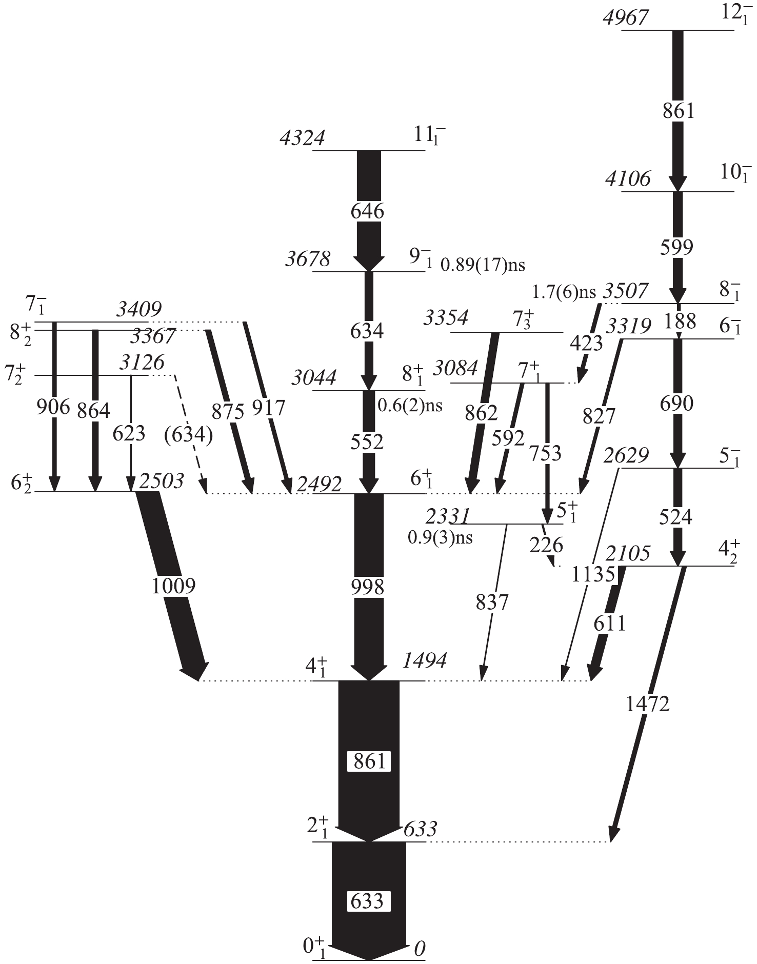Figure1. Partial level scheme for ¹⁰⁶Cd. The width of the arrows represents the relative intensities of the transitions. Relative intensity information was taken from Ref. [11]. Lifetimes of the 3678 keV 9$_{1}^{-}$ and 3044 keV 8$_{1}^{+}$ states were taken from Ref. [12], and lifetimes of the 3507 keV 8$_{1}^{-}$ and 2331 keV 5$_{1}^{+}$ states were taken from Ref. [19].

Figure2. Projections of the backward-backward matrix for a distance of 80 μm between the target and stopper foils.

The result in Ref. [5] was also reported in Ref. [12], and was obtained from the direct gating of the 861 keV 4$_{1}^{+}$ $\rightarrow$ 2$_{1}^{+}$ transition, but the contaminations from higher-lying transitions was not considered. Moreover, the level scheme of $^{106}$Cd presented in Ref. [12] did not exhibit the 862 keV 7$_{3}^{+}$ $\rightarrow$ 6$_{1}^{+}$ transition, but the 851 keV 7$_{3}^{+}$ $\rightarrow$ 6$_{2}^{+}$ transition, which was not seen in the present work by gating on the 1009 keV 6$_{2}^{+}$ $\rightarrow$ 4$_{1}^{+}$ and the 861 keV 4$_{1}^{+}$ $\rightarrow$ 2$_{1}^{+}$ transitions at $90^{\circ}$ (see Fig. 3). This 851 keV 7$_{3}^{+}$ $\rightarrow$ 6$_{2}^{+}$ transition was not found in Ref. [11]. If the 851 keV 7$_{3}^{+}$ $\rightarrow$ 6$_{2}^{+}$ transition exists, the unshifted component of the 851 keV transition will overlap with the backward shifted component of the 861 keV transitions, and the lifetime of the 2$_{1}^{+}$ state could not be determined by setting a cut on the backward shifted component of the 861 keV transitions.
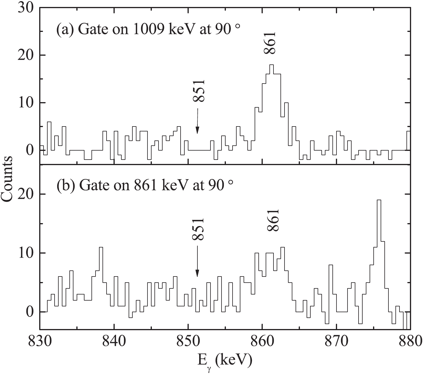Figure3. Background-corrected coincidence spectra obtained by gating on the (a) 1009 keV and (b) 861 keV $\gamma$-ray transitions at $90^{\circ}$. The 851 keV transition deexcited from the 3354 keV 7$_{3}^{+}$ state to 2503 keV 6$_{2}^{+}$ state in Ref. [12] cannot be seen in both spectra.

In order to subtract the contaminations, direct and indirect gating cases should be considered simultaneously. In the case of direct gating on the transition B, as shown in Fig. 4, the mean lifetime $\tau$ of the level L depopulated via transition A can be determined at every target to stopper distance x as:
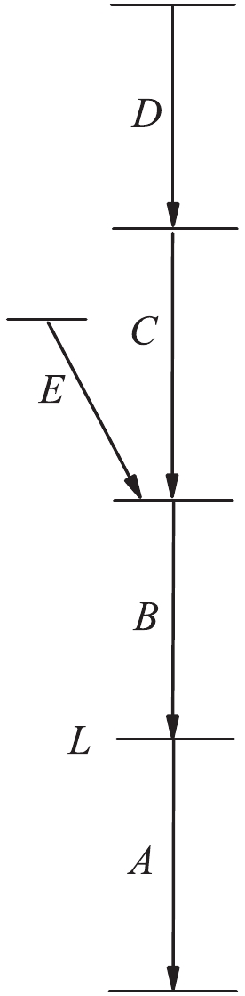Figure4. Level scheme sample for direct and indirect gating.

$ \begin{split} \tau_{L}(x) = \frac{I_{(u, s)}^{AB}}{\upsilon\cdot\dfrac{\rm d}{{\rm d}x}I_{(s, s)}^{AB}}\end{split},$

(1)

where $\upsilon$ is the recoil velocity, the subscripts s and u denote the Doppler shifted and unshifted components, respectively, and $I_{(u, s)}^{AB}$ refers to the normalized intensities I of the unshifted component of the depopulating transition A, obtained by gating on the shifted peak of transition B. When indirect gating is used, for example, when the gate is set on the shifted peak of transition C, the mean lifetime will transform into:

$\begin{split} \tau_{L}(x) = \frac{I_{(u, s)}^{AC}-\alpha\cdot I_{(u, s)}^{BC}}{\upsilon\cdot\dfrac{\rm d}{{\rm d}x}I_{(s, s)}^{AC}}\end{split},$

(2)

and

$\begin{split} \alpha = \frac{I_{(u, s)}^{AC}+I_{(s, s)}^{AC}}{I_{(u, s)}^{BC}+I_{(s, s)}^{BC}}.\end{split}$

(3)

If the energies of the $\gamma$-ray transitions B and C are the same, when a cut is set on the Doppler shifted component of transition B, a coincident gate will also be placed on the flight peak of transition C simultaneously. The shifted and unshifted components of transition A in the gated spectrum will contain two parts, one part is obtained by gating on the shifted part of transition B, and the other part is obtained from gating on the shifted part of transition C, as shown in Fig. 5.
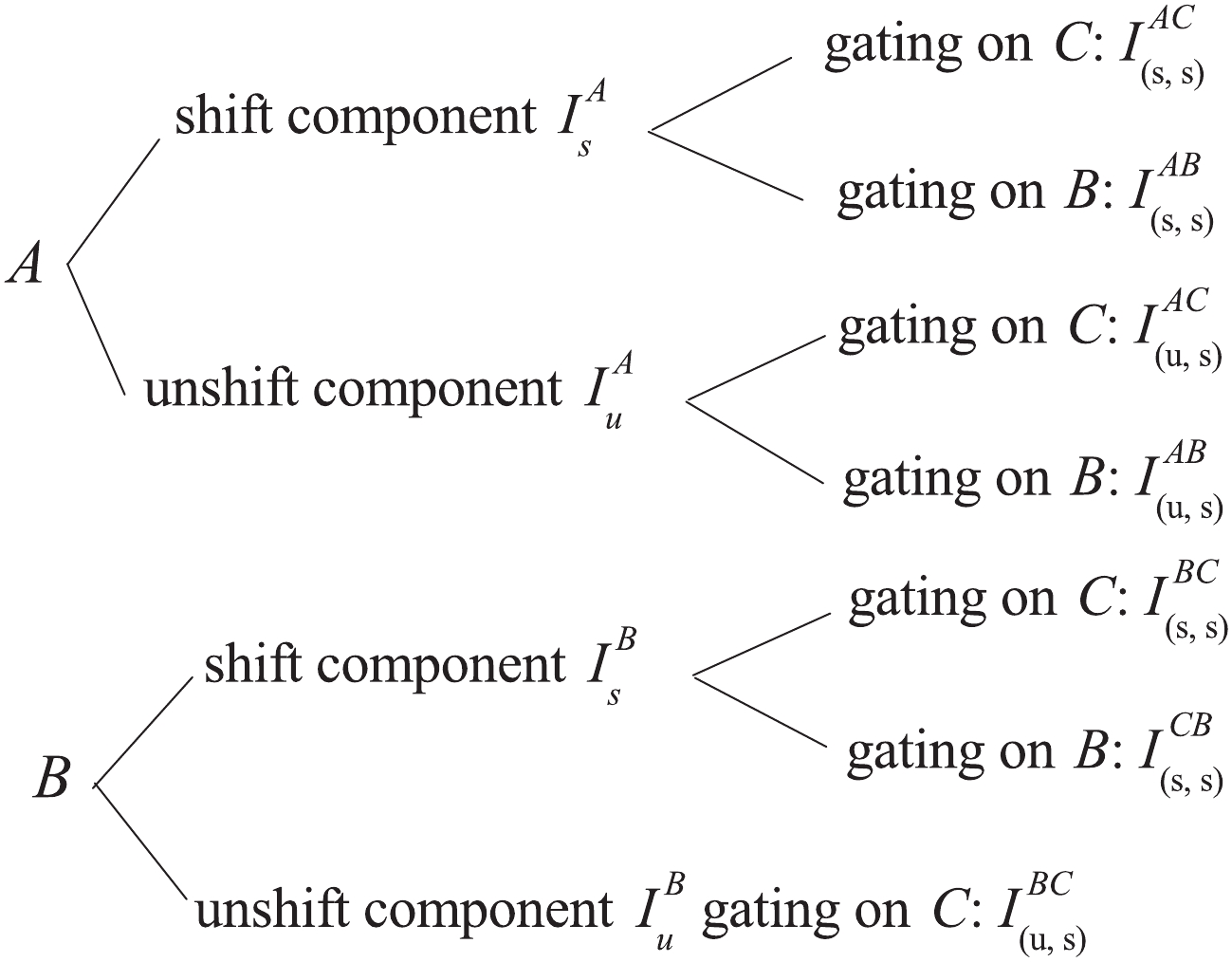Figure5. Shifted and unshifted components of transitions A and B in the gating spectrum.

$\left\{ \begin{split}&I_u^A = I_{(u,s)}^{AC} + I_{(u,s)}^{AB},\\&I_s^A = I_{(s,s)}^{AC} + I_{(s,s)}^{AB}.\end{split} \right.$

(4)

Though $I_{(u, s)}^{AC}$, $I_{(u, s)}^{AB}$, $I_{(s, s)}^{AC}$ and $I_{(s, s)}^{AB}$ could not be identified in the gating spectrum, the lifetimes of level L derived from the gating on transitions C and B should be the same, which means:

$ \begin{split} \tau_{L}(x) = \frac{I_{(u, s)}^{AC}-\alpha\cdot I_{(u, s)}^{BC}}{\upsilon\cdot\dfrac{\rm d}{{\rm d}x}I_{(s, s)}^{AC}} = \frac{I_{(u, s)}^{AB}}{\upsilon\cdot\dfrac{\rm d}{{\rm d}x}I_{(s, s)}^{AB}}.\end{split}$

(5)

The following relations can be obtained from Eqs. (4) and (5):

$\begin{split} \frac{\rm d}{{\rm d}x}I_{(s, s)}^{AB} =& \frac{\rm d}{{\rm d}x}(I_s^A-I_{(s, s)}^{AC}) \\ =& \frac{\rm d}{{\rm d}x}I_s^A-\frac{\rm d}{{\rm d}x}I_{(s, s)}^{AC}, \end{split}$

(6)

$\left\{ \begin{split}&\frac{\rm d}{{{\rm d}x}}I_{(s,s)}^{AB} = \frac{{I_{(u,s)}^{AB}}}{{\upsilon \cdot {\tau _L}}} = \frac{{I_u^A - I_{(u,s)}^{AC}}}{{\upsilon \cdot {\tau _L}}},\\&\frac{\rm d}{{{\rm d}x}}I_{(s,s)}^{AC} = \frac{{I_{(u,s)}^{AC} - \alpha \cdot I_{(u,s)}^{BC}}}{{\upsilon \cdot {\tau _L}}},\end{split} \right.$

(7)

then

$ \frac{I_u^A-I_{(u, s)}^{AC}}{\upsilon\cdot\tau_{L}} = \frac{\rm d}{{\rm d}x}I_s^A-\frac{I_{(u, s)}^{AC}-\alpha\cdot I_{(u, s)}^{BC}}{\upsilon\cdot\tau_{L}}.$

(8)

$I_u^{AC}$ can be cancelled, and Eq. (8) is transformed into:

$\begin{split} \tau_{L}(x) = \frac{I_u^A-\alpha\cdot I_{(u, s)}^{BC}}{\upsilon\cdot\dfrac{\rm d}{{\rm d}x}I_s^A}.\end{split}$

(9)

The form of Eq. (9) is similar to Eq. (2). However, in Eq. (9), gates are set on direct and indirect transitions simultaneously, and the shifted and unshifted peaks of transition A in the gating spectrum contain direct and indirect gating components. A problem arises due to the factor of proportionality $\alpha$, which is determined by the detector efficiencies and angular correlations [16]. In the present work, the numerator can not be extracted from the experimental data as shown in Eq. (3). Thus, the factor $\alpha$ was replaced as:

$\alpha = \frac{\varepsilon_A\cdot\omega_{AC}(\theta)}{\varepsilon_B\cdot\omega_{BC}(\theta)},$

(10)

where $\varepsilon_A$ and $\varepsilon_B$ are the detection efficiencies of transitions A and B, respectively, and $\omega_{AC}(\theta)$ is the angular correlation between transitions C and A at angle $\theta$, respectively.
If there are more than one contaminations, say transition E shown in Fig. 4, whose energy is the same as that of transition B, but transition C and E is not coincident with each other, Eq. (9) and Eq. (10) still hold. The biggest difference between Eq. (9) and Eq. (2) is that the factor of proportionality $\alpha$ in Eq. (9) could not be extracted from experimental data easily. However, it can be chosen in another way: a gate was set on the unshifted component of a transition which is coincident with the 4$_{1}^{+}$ $\rightarrow$ 2$_{1}^{+}$ 861 keV transition and the 2$_{1}^{+}$ $\rightarrow$ 0$_{1}^{+}$ 633 keV transition, but not coincident with the 7$_{3}^{+}$ $\rightarrow$ 6$_{1}^{+}$ 862 keV transition and the 12$_{1}^{-}$ $\rightarrow$ 10$_{1}^{-}$ 861 keV transition. The ratio of the intensities of the 633 keV and 861 keV transitions in the gating spectra can be used as the factor of proportionality $\alpha$. In the present work, a gate was set on the 7$_{1}^{-}$ $\rightarrow$ 6$_{2}^{+}$ 906 keV transition and the 7$_{1}^{-}$ $\rightarrow$ 6$_{1}^{+}$ 917 keV $\gamma$-ray, respectively. The values of $\alpha$ extracted by different gating transitions were found to be consistent, and a mean value $\alpha$ = 1.35 (18) was used in the present work.
It should be noted that Eq. (2) is used to calculate the lifetime of level L, which is fed by a single elementary transition directly [15]. But in the present work, the 2$_{1}^{+}$ state is fed by several transitions. The 10$_{1}^{-}$ 4106 keV state decays to the 2$_{1}^{+}$ 633 keV state via several paths except the 4$_{1}^{+}$ $\rightarrow$ 2$_{1}^{+}$ 861 keV transition, e.g., the 4$_{2}^{+}$ $\rightarrow$ 2$_{1}^{+}$ 1472 keV transition. The influence of the 1472 keV transition could be estimated by subtracting all decay paths that decay to the 4$^+_1$ state, such as the 423 keV, 827 keV, 1135 keV, and 611 keV transitions deexciting from the 8$^-_1$, 6$^-_1$, 5$^-_1$ and the 4$^+_2$ states, respectively. In addition, only 10% intensities of 12$^-_1$ $\rightarrow$ 10$^-_1$ 861 keV transitions decay to the 2$^+_1$ state through the 4$^+_2$ $\rightarrow$ 2$^+_1$ 1472 keV transition. These intensities have been taken into account in the statistical error.
It is necessary to modify the recoil velocity in the data analysis, because of the low recoil velocities of the compound nucleus. In the present data analysis, three 1 keV wide cuts were set on the Doppler-shifted parts of the 861 keV $\gamma$-peaks, from 852 keV to 855 keV. These spectra are shown in the upper three spectra of Fig. 6. It can be seen clearly from the shifted peak positions of these three spectra that the mean recoil velocities of the compound nuclei are from 0.0085 to 0.0105 c. The sum gate of these three cuts was used to determine the mean velocity of the recoil nucleus, and it is demonstrated in the bottom of Fig. 6. The mean recoil velocity 0.00905 $\dfrac{v}{c}$ was used in the present work. The spread of the recoil velocity $\dfrac{\Delta v}{c}$ is almost 0.01%. This spread has been added in the statistical error as a systematic error.
Figure6. (color online) Projection of the backward-shifted 633 keV peak in $^{106}$Cd from gating on the shifted components of the 861 keV $\gamma$ peak. The range of the $\gamma$-ray coincidence condition is shown in the upper center of each spectrum. The dashed line denotes the measured centroid of the Doppler-shifted peak.

Eq. (9) and Eq. (10) were used to fit curves of the shifted and unshifted normalized intensities by the NAPATAU program [20]. The intensities of the $\gamma$ peaks at every target-to-stopper distance should be normalized by setting gates on both the Doppler-shifted and unshifted parts of the 861 keV 4$_{1}^{+}$ $\rightarrow$ 2$_{1}^{+}$ $\gamma$ transition. Then, sum intensities of the unshifted and shifted parts of the higher lying 1009 keV 6$_{2}^{+}$ $\rightarrow$ 4$_{1}^{+}$ $\gamma$ transition were determined. These intensities were normalized to the intensity whose target-to-stopper distance is 30 μm. A 3 keV wide gate was placed form 852 to 855 keV, which is the backward shifted part of the 861 keV transitions. The backward shifted and unshifted spectra of the 633 keV 2$_{1}^{+}$ $\rightarrow$ 0$_{1}^{+}$ transition and corresponding unshifted components of the 861 keV transitions were fitted and plotted in Fig. 7. The final decay curves and the $\tau$ plot are shown in Fig. 8. It should be noted that the unshifted intensities in the bottom panel of Fig. 8 were obtained by reducing the unshifted peaks of the 861 keV $\gamma$-ray in the right side of Fig. 7 from the unshifted peaks of the 633 keV transition in the left side of Fig. 7 with a factor of proportionality $\alpha$. From the resulting decay curves, the deduced mean-lifetime of the 2$_{1}^{+}$ state in $^{106}$Cd is 9.9(12) ps. Limited by the low detective ability, the error in the present work is mainly influenced by the poor statistics of the experimental data.
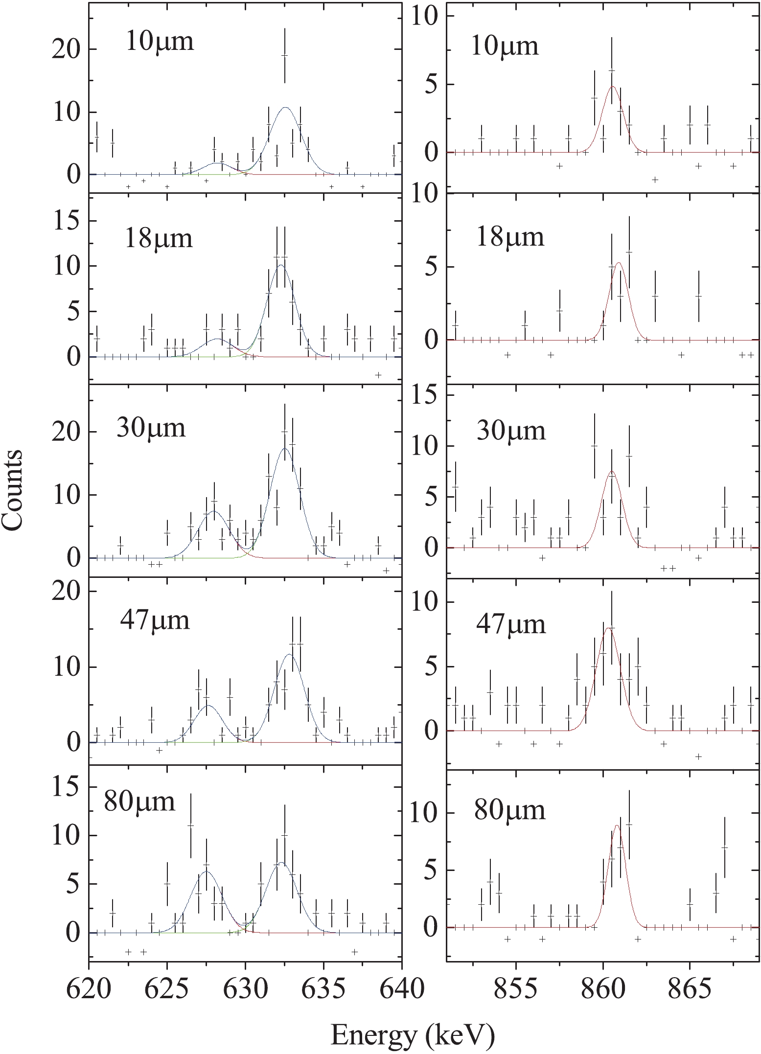Figure7. (color online) (left) Projected stopped and backward-shifted components for the 633 keV, 2$_{1}^{+}$ $\rightarrow$ 0$_{1}^{+}$ transition in $^{106}$Cd from gating on the backward-shifted components of the 861 keV. (right) Corresponding backward-unshifted components of 861 keV transition.

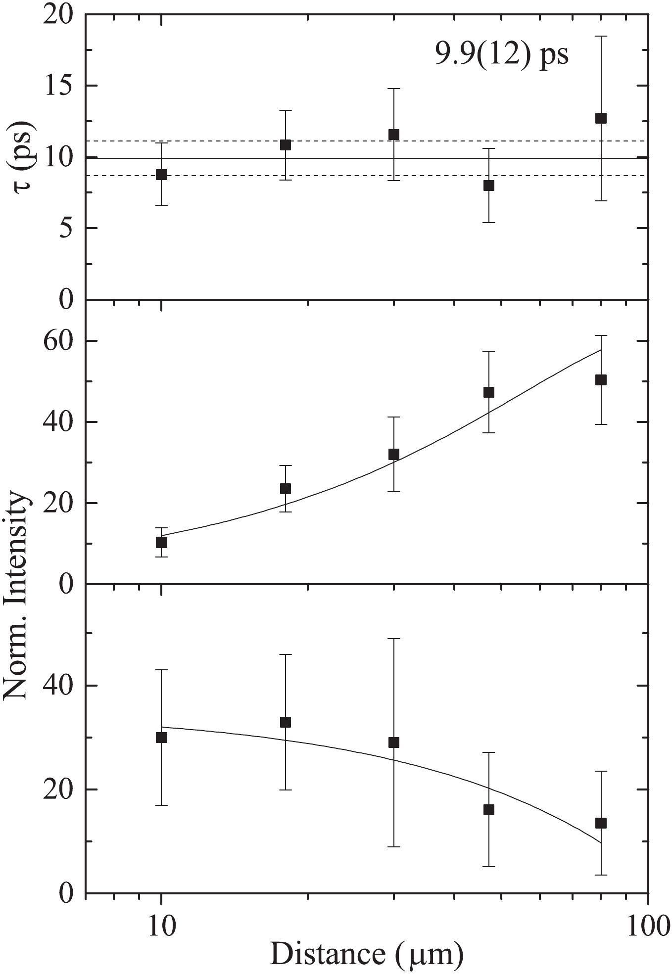Figure8. Decay curves and lifetime determination of the 633 keV, 2$_{1}^{+}$ $\rightarrow$ 0$_{1}^{+}$ transition in $^{106}$Cd. The middle and lower panel show the Doppler-shifted and stopped intensities vs distance. The mean-lifetime at each distance is determined (using Eq. (9) and Eq. (10)), and is shown in the upper panel as a function of the distance. The weighted average of these values yields the overall mean-lifetime.

By reducing the contamination, the lifetime $\tau$ = 9.9(12) ps determined in this study is shorter and more reasonable than the result deduced by the DDCM in Ref. [5]. This value fits well with the adopted value 10.49(12) ps [2] within the experimental uncertainty. The reported value of7.0(3) ps in Ref. [4] for the $2_{1}^{+}$ state in $^{106}$Cd is 33% shorter than the evaluated value in the NNDC [6]. The difference may be caused by the influence of the long-live state above, i.e., the lifetime of the $4_{2}^{+}$ state reported in Ref. [4] is longer than 10 ps, though the lifetime of this state evaluated by the NNDC is $\leqslant$ 2.9 ps.
The lifetime of $\tau$ = 9.9(12) ps for the $2_{1}^{+}$ state measured in this study yields a reduced transition probability of $B(E2; 2_{1}^{+} \rightarrow 0_{1}^{+})$ = 0.081(10) ${\rm e}^2{\rm b}^2$, or 27.2(33) W.u.. The $B(E2)$ value is compared to those of neighboring even-even Cd isotopes in Fig. 9. Though cadmium isotopes are only two proton holes away from the Z = 50 number, this comparison of the $B(E2)$ values illustrates that the collectivity of the 2$_{1}^{+}$ states increases rapidly with an increasing neutron number from $^{102}$Cd to $^{106}$Cd. However, the increasing trend of experimental results slows down from $^{106}$Cd to $^{110}$Cd, which means that the collectivity or the deformation of the ground states in $^{106}$Cd, $^{108}$Cd, and $^{110}$Cd are similar. $^{106}$Cd and $^{108}$Cd were both predicted to exhibit features of E(5) critical-point symmetry [1]. This trend may confirm the prediction to some extent. The $B(E2)$ value obtained in the present measurement fits smoothly into the systematic trend. It should be noted that the new $B(E2)$ values of $^{102,104}$Cd in Fig. 9 were taken from Ref. [9] instead of Ref. [7].
Figure9. (color online) Systematics of $B(E2)$ values in W.u. for the excited 2$_{1}^{+}$ states in the even Cd isotopes. The existing experimental data for $^{106}$Cd in Refs. [4, 5] and the present work are presented in comparison with evaluated values in NNDC and the shell model (SM) calculations [9]. Evaluated values are taken from $^{102,104}$Cd [9], $^{106,108}$Cd [2], $^{110}$Cd [21], $^{112}$Cd [22].

Several shell model calculations for light cadmium isotopes have been performed in Refs. [4, 7-10]. The theoretical $B(E2)$ values show a smooth increase from $^{102}$Cd to $^{106}$Cd, which fit well with the experimental results (see Fig. 9). For $^{106}$Cd, the theoretical prediction $B(E2)$ value would result in a better agreement from the effective charge $(e_\pi, e_\nu)$ = (1.6e, 1.0e) [9], rather than (1.7e, 1.1e) [8, 10] (see Table 1 and Fig. 9). The transition probability of $B(E2; 2_{1}^{+} \rightarrow 0_{1}^{+})$ = 0.081(10) ${\rm e}^2{\rm b}^2$ from the present work also fits close to the shell model calculated result of 0.083 ${\rm e}^2{\rm b}^2$ in Ref. [4].

references	$\tau$/ps	inert core	proton orbits	neutron orbits	effective charge $(e_\pi, e_\nu)$	$B(E2)/({\rm e}^2{\rm b}^2)$
						exp	cal
This work	9.9(12)					0.081(10)
M. T. Esat et al. [2]	10.49(12)					0.0765(9)
S. K. Chamoli et al. [3]	9.8					0.082
S. F. Ashley et al. [5]	16.4(9)					0.049(3)
N. Benczer-Koller et al. [4]	7.0(3)	$^{78}_{28}$Ni$_{50}$	$f_{5/2}$, $p_{3/2}$, $p_{1/2}$, $g_{9/2}$	$g_{7/2}$, $d_{5/2}$, $d_{3/2}$, $s_{1/2}$	(1.75e, 0.75e)	0.115(8)	0.061
				$g_{7/2}$, $d_{5/2}$, $d_{3/2}$, $s_{1/2}$	(2.0e, 1.0e)		0.097
				$g_{7/2}$, $d_{5/2}$, $d_{3/2}$	(1.75e, 0.75e)		0.052
				$g_{7/2}$, $d_{5/2}$, $d_{3/2}$	(2.0e, 1.0e)		0.083
N. Boelaert et al. [7, 8] T. Schmidt et al. [10]		$^{88}_{38}$Sr$_{50}$	$p_{1/2}$, $g_{9/2}$	$d_{5/2}$, $s_{1/2}$, $d_{3/2}$, $g_{7/2}$, $h_{11/2}$	(1.7e, 1.1e)		0.0883
A. Ekstrom [9]		$^{88}_{38}$Sr$_{50}$	$p_{1/2}$, $g_{9/2}$	$d_{5/2}$, $s_{1/2}$, $d_{3/2}$, $g_{7/2}$, $h_{11/2}$	(1.6e, 1.0e)		0.076

Table1.Comparisons of lifetimes and $B(E2)$ values of the 2$_{1}^{+}$ state in $^{106}$Cd in different experimental (exp) results and different shell model calculations (cal).

The excitation energy ratio $R_{4/2}$, defined as $E(4_{1}^{+})$/$E(2_{1}^{+})$, for $^{106}$Cd is 2.36. This value is predicted to be 2.00 for a spherical harmonic vibrator, 2.50 for a $\gamma$-soft rotor, and 3.33 for an ideal rotor. Though the $R_{4/2}$ ratio implies that the yrast band in $^{106}$Cd is a little far away from the E(5) prediction 2.20, it is still found within the range of 2.00< $R_{4/2}$$\leqslant$2.40 [1]. In addition, the $B_{4/2}$ value, defined as $B(E2; 4_{1}^{+} \rightarrow 2_{1}^{+})$/$B(E2; 2_{1}^{+} \rightarrow 0_{1}^{+})$, is 1.65(31) in the present work (the $B(E2; 4_{1}^{+} \rightarrow 2_{1}^{+})$ value was taken from Refs. [6, 23]). This ratio is predicted to be 2.0 for a geometric vibrator, and 1.43 for a symmetric rotor. Though the $B_{4/2}$ ratio is close to the the E(5) prediction 1.56 [1], it is hard to identify the E(5) critical-point symmetry in $^{106}$Cd clearly, because most of the low spin state lifetimes in Ref. [4] are different from the NNDC values (see TABLE II in Ref. [4]). More experiments are required to clarify the differences of these short lifetimes.

The mean lifetime of the 2$_{1}^{+}$ state in $^{106}$Cd was remeasured in the present investigation. By subtracting the contaminations, the result 9.9(12) ps deduced from the RDDS technique and the DDCM is well within the experimental uncertainty of the evaluated value 10.49(12) ps [2], and it is more reasonable than the reported value in Ref. [5], which is also measured by the RDDS technique in combination with DDCM. The reduced transition probability $B(E2)$ in our work, which fits smoothly into the systematic trend, is 0.081(10) ${\rm e}^2{\rm b}^2$. This result can be explained by the shell model calculations.
The authors would like to thank the crew of the HI-13 tandem accelerator at the China Institute of Atomic Energy for steady operation of the accelerator. We are also grateful to Dr. Q. W. Fan for preparing the target.