Shao-Fei Chen
, Bo-Chao Liu ^,
,

Corresponding author: Bo-Chao Liu, liubc@xjtu.edu.cn

School of Science, Xi’an Jiaotong University, Xi’an 710049, China
Received Date:2019-11-01
Available Online:2020-03-01
Abstract:We investigate the $ K^* $ production in the $ KN\to K \pi p $ reaction using the effective Lagrangian approach and the isobar model. To describe this reaction, we first take into account the contributions from the $ \pi $, $ \rho $ and $ \omega $ exchanges, as in previous studies. We find that although the experimental data can be generally described, there are some obvious discrepancies between the model and the experiments. To improve the model, we consider the contributions of the axial-vector meson and hyperon exchange. It is shown that a large contribution of the axial-vector meson exchange can significantly improve the results. This may indicate that the coupling of the axial-vector meson, e.g. $ a_1(1260) $, is large in the $ KK^* $ channel. To verify our model, measurements of the angular distributions and spin density matrix elements of $ K^{*0} $ in the $ K_{\rm L} p\to K^{*0} p $ reaction would be helpful, and we make predictions for this reaction for a future comparison.

HTML

--> --> -->

The $ KN $ interactions constitute an important sector of the studies of strong interactions. Due to the positive strangeness of the $ KN $ system, their interactions have some special features. One example is that no 3-quark state can be formed in the $ KN $ channel, which has attracted a lot of interest in finding the pentaquark state $ \Theta $(or $ Z^* $ in the old literature) in $ KN $ interactions. Even though there is still no clear evidence for the existence of the pentaquark state in this channel [1-7], the proposed measurements of the $ K^+d $ interactions [8] at J-PARC are expected to provide a further test for the existence of $ \Theta $. Besides the search for the pentaquark state, the studies of resonance production in the $ KN $ scattering reactions are also relevant. Even though the resonance states have not been found in the $ KN $ elastic scattering, they can be produced in the inelastic processes in at least a three-body final state. In fact, the $ K^+N $ or $ K_{\rm L}N $ scattering processes were widely used for investigating the properties of hadron resonances during the 1960’s and 1970’s [9]. It is known that resonance production processes usually dominate these scattering processes in the resonance region. This feature makes these reactions suitable for investigating the properties of hadron resonances. Although such studies started a few decades ago, the understanding of these reactions is still not satisfactory. Due to the low statistics of the available experimental data and the absence of new data, the relevant studies almost ceased in the past decade. Recently, it was proposed to use the secondary $ K_{\rm L} $ beam to perform the $ K_{\rm L} N $ scattering experiments at Jefferson Lab [10]. If such experiments could be done in the future, the obtained data would certainly prompt relevant studies and help clarify some problems in understanding the $ KN $ interactions. From the theoretical side, it is hence meaningful to recheck the previous studies and look for new perspectives and physical motivations for studying the relevant $ K_{\rm L} N $ scattering processes.
In this paper, we analyze the $ K^* $ production in the $ KN\to K \pi p $ reaction using the effective Lagrangian approach and the isobar model. It was shown that this reaction is dominated by the production of $ K^* $ and $ \Delta(1232) $ resonances in the low energy region, and the contributions of these two resonances could be separated [11]. Thus, this reaction offers a possibility to study the $ K^* $ production mechanism in $ KN $ interactions. Previous analysis of this reaction was mainly focused on relatively high energies, and it was assumed that the reaction is dominated by the $ \pi $, $ \omega $ and $ \rho $ exchange. In Refs. [12, 13], it was argued that $ K^*N $ is produced partly via pion exchange and partly via vector meson exchange, and that with energy decrease the pion exchange contribution gradually increases. In a later analysis [11, 14], the authors concluded that the reaction is dominated by vector meson exchange down to threshold, and no evidence of a significant increase of pseudoscalar exchange at low energy was seen. The same reaction was also studied in Ref. [15], and it was concluded that the $ \omega $ exchange does not play any role in this reaction, in contrast to the results in Refs. [11-14]. However it seems that the parameters of the models [11, 12, 15] are not compatible with the values in recent literature. Therefore, further studies are required. In the present work, we first consider the contribution of the $ \pi $, $ \rho $ and $ \omega $ exchange, as in previous works. We fix the parameters that are relatively well-known in literature, while the others are fitted to the experimental data as free parameters. We find that although the experimental data can be generally described, there are some obvious discrepancies between the model and the experiments. The natural way to resolve the issue is to include in the model some other mechanism, e.g. hyperon and axial-vector meson exchange. In fact, we find that the inclusion of the axial-vector meson exchange can significantly improve the model, while the hyperon exchange does not seem important. Among the various axial-vector mesons, we focus on the role of $ a_1(1260) $(hereafter referred to as $ a_1 $). Contrary to other axial-vector mesons, the branching ratio for the decay $ a_1\to K^*K $ was measured [16]. The $ a_1NN $ coupling can be estimated due to its role in the $ NN $ axial-vector coupling [17]. Other axial-vector mesons, such as $ f_1(1285) $ or $ b_1(1235) $, may also give a contribution. However, we do not consider them explicitly since their couplings to the $ NN $ and $ KK^* $ channels are unknown. It should be mentioned that the $ \eta $ exchange is also allowed in this reaction. We do not consider it, since its contribution is expected to be small due to the vanishing $ \eta NN $ coupling [18]. To verify our model, it would be helpful to test its predictions for the $ K_{\rm L} N\to K^* N $ reaction. As shown below, various models give distinct predictions for this reaction. Thus, the measurements at JLab could provide valuable information about the reaction mechanism.
This article is organized as follows. In Sec. 2, we present the theoretical formalism used in the calculations. Numerical results and discussion are presented in Sec. 3, followed by a summary in the last section.

In this work, we study the following two reactions:

$ \begin{split}(a) \quad K^+ p \to pK^{*+}( \to K^0 \pi^+), \\ (b)\quad K^+ n \to pK^{*0}( \to K^+ \pi^-). \end{split} $

The $ K^* $ production in the two reactions can be described by the Feynman diagrams shown in Fig. 1. It includes the $ t- $channel $ \pi $, $ \rho $, $ \omega $, $ a_1 $ exchange terms and the $ u- $channel $ \Lambda $, $ \Sigma $ exchange terms. To compute these contributions, the following interaction Lagrangian densities are needed [19-23]:
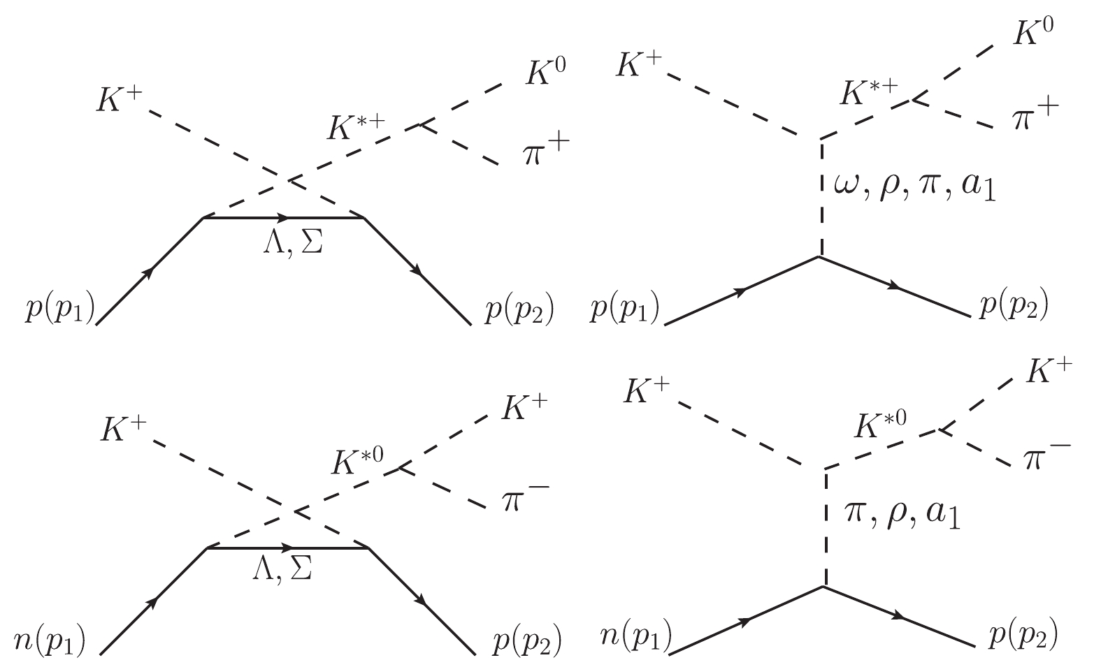Figure1. Model of the reactions $ K^+ p \to K^{*+} p \to K^0 \pi^+ p $ and $ K^+ n \to K^{*0} p \to K^+ \pi^- p $. $ p_1 $ and $ p_2 $ are the four-momenta of the initial and final nucleons.

$ \begin{split} {\cal L}_{K^* K \pi} = & {\rm i} G_V\{(\partial_\mu{\bar{K}})\vec{\tau}K^{*\mu}\cdot\vec{\pi} -{\bar{K}}\vec{\tau}K^{*\mu}\cdot(\partial_\mu\vec{\pi})\}+{h.c.}, \end{split} $

(1)

$ \begin{split} {\cal L}_{K^* K V} =& g_{K^*K V}\varepsilon^{\mu\nu\alpha\beta} (K^-\partial_{\alpha}K^{*+}_\beta\partial_{\mu}V_\nu \\ & +K^+\partial_{\mu}K^{*-}_\nu\partial_{\alpha}V_\beta), \end{split} $

(2)

$ \begin{array}{l} {\cal L}_{NNV} = -g_{NNV}\bar{N}\left(\gamma_\mu-\dfrac{k_V}{2 m_N}\sigma_{\mu\nu}\partial^\nu\right)V^\mu N , \end{array} $

(3)

$ \begin{split} {\cal L}_{NY K^*} = -g_{NY K^*}\bar{N}\left(\gamma_\mu Y K^{*\mu}-\frac{\kappa_{Y}}{2m_N}\sigma_{\mu\nu}Y\partial^{\nu}K^{*\mu}\right) +{h.c.}, \end{split} $

(4)

$ \begin{array}{l} {\cal L}_{NYK} = -g_{NYK}\bar{N}\gamma_5 Y K+{h.c.}, \end{array} $

(5)

$ \begin{array}{l} {\cal L}_{NN\pi} = -{\rm i} g_{NN\pi}\bar N \gamma_5 \vec{\tau}\cdot\vec{\pi} N, \end{array} $

(6)

where V indicates the vector meson $ \rho $ or $ \omega $, and Y represents $ \Lambda $ or $ \Sigma $. The $ \sigma_{\mu\nu} $ in Eqs. (3) and (4) is defined as

$ \begin{split} \sigma_{\mu\nu} = \frac{\rm i}{2}(\gamma_\mu\gamma_\nu-\gamma_\nu\gamma_\mu). \end{split} $

(7)

The coupling constants in the Lagrangians can be determined either by extracting them from the experimental data or by predictions of theoretical models. In Tables 1 and 2, we list the values of the coupling constants used in this work.

vertex	CD-Bonn model [24]
	g[$ \kappa $]	$ \Lambda_\alpha $/GeV
$ NN\omega $	15.85(0.0)	1.5
$ NN\rho $	3.25(6.1)	1.31
$ NN\pi $	13.07	1.72

Table1.Parameters of the N-N-meson vertices.

vertex	$ g_{ { {{K^*KM}}}} $	Ref.	vertex	g($ \kappa $)	Ref.
$ KK^*\rho $	7.45 GeV?1	[25]	$ NK\Lambda $	?13.24	[21]
$ KK^*\omega $	7.45 GeV?1	[25]	$ NK\Sigma $	3.58	[21]
$ KK^*\pi $	3.02	[26]	$ NK^*\Lambda $	?4.26 (2.66)	[27]
			$ NK^*\Sigma $	?2.46 (?0.47)	[27]

Table2.Coupling constants of the K^*-K-meson and K^*(K)-N-Y vertices used in this work.

The general invariant scattering amplitude for the reactions under study can be written as

$ \begin{array}{l} {\cal M}_i = \bar u(p_2)\; {\cal A}_i\; u(p_1), \end{array} $

(8)

where i denotes the various exchanged particles. $ \bar u(p_2) $ and $ u(p_1) $ are the spinors of the outgoing and incoming nucleons, respectively. With the effective Lagrangian densities given above, one can, for example, easily construct $ {\cal A}_i $ for the $ K^+ p \to K^{*+} p \to K^0 \pi^+ p $ reaction as

$ \begin{split} {\cal A}_V =& \sqrt{2}G_V\; g_{NNV}g_{KK^*V} \frac{-p^{K^0}_\nu+p^{\pi^+}_\nu}{p_{K^*}^2-m_{K^*}^2+{\rm i} m_{K^*}\Gamma}\varepsilon^{\mu\nu\alpha\beta} \\ &\times p^{K^*}_\mu p^V_\alpha\frac{1}{p_V^2-m_V^2} \left(\gamma_\beta-{\rm i} \frac{k_V}{2m_N}\sigma_{\beta\gamma}p^\gamma\right), \end{split} $

(9)

$ \begin{split} {\cal A}_Y =& {\rm i} \sqrt{2}G_Vg_{YNK}g_{K^*NY}\gamma_5(-p^\alpha_{\pi^+}+p^\alpha_{K^0}) \frac{{\not\!\!\!p }_Y+m_Y}{p^2_Y-m^2_Y} \\&\times \frac{-g_{\mu\alpha}+\frac{p_\mu^{K^*}p_\alpha^{K^*}}{m^2_{K^*}}}{p^2_{K^*}-m^2_{K^*}+im_{K^*}\Gamma} \left(\gamma^\mu-{\rm i}\frac{\kappa_{Y}}{2m_N}\sigma^{\mu\nu}p_\nu^{K^*}\right), \end{split} $

(10)

$ \begin{split} {\cal A}_P =& g_{NNP}\sqrt{2}G_V g_{K^*KP}(p_{K^0}^\mu-p_{\pi^+}^\mu) \\ &\times \frac{-g_{\mu\nu}+\frac{p^{K^*}_\mu p^{K^*}_\nu}{p_{K^*}^2}}{p_{K^*}^2-m_{K^*}^2+{\rm i} m_{K^*}\Gamma}\cdot\frac{p_{k^+}^\nu-p_P^\nu}{p_P^2-m_P^2}\gamma_5, \end{split} $

(11)

where the subscript V (vector meson), Y (hyperon) and P (pseudoscalar meson) stand for the corresponding exchanged particles. The width of $ K^* $ is taken as $ \Gamma = 50.8 $ MeV and the coupling constant $ G_V = 3.02 $ [26] is used in the calculations.
To take into account the finite extension of hadrons, we also introduce the form factors in the amplitudes. For the N-N-meson vertex, we adopt the form factors used in the Bonn model [24],

$ \begin{array}{l} F^\alpha_N(q_{\rm ex}^2,M_{\rm ex}) = \dfrac{\Lambda_\alpha^2-M_{\rm ex}^2}{\Lambda_\alpha^2-q_{\rm ex}^2}\, , \end{array} $

(12)

where $ \Lambda_\alpha $ takes the values shown in Table 1. For the hyperon exchange vertex, we use the following form factor [20, 21, 28],

$ \begin{split} F_Y(q_{\rm ex}^2,M_{\rm ex}) = {\Lambda^4_Y\over \Lambda^4_Y+(q_{\rm ex}^2-M_{\rm ex}^2)^2}\, , \end{split} $

(13)

where Y is $ \Lambda $ or $ \Sigma $. For the $ K^* $-K-meson vertex, we take the following form factor [19]

$ \begin{array}{l} F^\alpha_{K^*}(q_{\rm ex}^2,M_{\rm ex}) = \dfrac{{\Lambda^{*}_\alpha} ^2-M_{\rm ex}^2}{{\Lambda^{*}_\alpha}^2-q_{\rm ex}^2}\, . \end{array} $

(14)

In the above formulae, $ q_{\rm ex} $ and $ M_{\rm ex} $ are the 4-momentum and mass of the exchanged particle. The index $ \alpha $ can be $ \pi $, $ \rho $, $ \omega $ and $ a_1 $, denoting the corresponding exchanged particles. The cutoff parameter $ \Lambda_\alpha $ is taken from the Bonn model (see Table 1). $ \Lambda_Y $ and $ \Lambda^*_\alpha $ are free parameters since they are not well constrained in previous studies.
The differential cross-section for this reaction can be represented by

$ \begin{split} {\rm d}\sigma =& {m_N \over 4F}\sum\limits_{s_i}\sum\limits_{s_f}|{\cal M}|^2{m_N {\rm d}^3p_2 \over E_2}{{\rm d}^3p_{K} \over E_{K}}{{\rm d}^3p_{\pi} \over E_{\pi}} \\ & \times\delta^4(p_1+p_{K^+}-p_2-p_{K}-p_{\pi}), \end{split} $

(15)

where $ F = (2\pi)^5 \sqrt{(p_1\cdot p_{K^+})^2-m_N^2m_{K^+}^2} $ and $ {\cal M} $ is the full amplitude.
The spin density matrix elements (SDMEs) of $ K^* $ can be extracted by analyzing the angular distributions of its decay products, which offer valuable information about the reaction mechanism. SDMEs can be defined as

$ \begin{split} \rho_{ { {{mm'}}}} = \frac{\displaystyle\sum\limits_{ { {{s_i,s_f}}}}M(K^+p_{ { {{s_i}}}}\to K^*_{ { {{m}}}}p_{ { {{s_f}}}})M^*(K^+p_{ { {{s_i}}}}\to K^{*}_{ { {{m'}}}}p_{ { {{s_f}}}})}{\displaystyle\sum\limits_{ { {{s_i,s_f,m}}}}|M(K^+p_{ { {{s_i}}}}\to K^{*}_{ { {{m}}}}p_{ { {{s_f}}}})|^2},\\ \end{split} $

(16)

where $ s_i $, $ s_f $ and m denote the spin polarization of the corresponding particles. Using Eq. (16) to calculate SDMEs, we treat the reaction as a quasi two-body process, i.e. $ K^+ p\to K^* p $, and ignore the decay of $ K^* $^①. Note that to describe the spin polarization of $ K^* $ there are three kinds of quantum axes used in literature: the s-channel helicity frame (Helicity frame), the t-channel helicity frame (Gottfried-Jackson frame), and the Adair frame. These three frames are not independent and can be related through frame transformations [29, 30]. In the present study, we consider the Helicity frame and Gottfried-Jackson frame, since the experimental data for these two frames are available [31]. In this work, we follow the conventions in Ref. [30].

With the formulae presented in the last section, the full amplitude can be written as

$ \begin{split} {\cal M} =& {\cal M}_\omega + {\rm e}^{{\rm i}\phi_\pi} {\cal M}_\pi+ {\rm e}^{{\rm i}\phi_\rho} {\cal M}_\rho + {\rm e}^{{\rm i}\phi_\Lambda} {\cal M}_\Lambda \\&+ {\rm e}^{{\rm i}\phi_\Sigma} {\cal M}_\Sigma+ {\rm e}^{{\rm i}\phi_{a_1}} {\cal M}_{a_1}, \ \end{split} $

(17)

for the reaction $ K^+ p \to K^{*+} p \to K^0 \pi^+ p $ and

$ \begin{array}{l} {\cal M} = 2{\rm e}^{{\rm i}\phi_\pi}{\cal M}_\pi+2 {\rm e}^{{\rm i}\phi_\rho} {\cal M}_\rho+ {\rm e}^{{\rm i}\phi_\Lambda} {\cal M}_\Lambda - {\rm e}^{{\rm i}\phi_\Sigma} {\cal M}_\Sigma+2 {\rm e}^{{\rm i}\phi_{a_1}} {\cal M}_{a_1}, \ \end{array} $

(18)

for the reaction $ K^+ n \to K^{*0} p \to K^+ \pi^- p $. The relative phases among the amplitudes are introduced since they should in general be complex, and in a model based on tree-level calculations the relative phases cannot be determined^②. Thus, it is better to set them as free parameters and examine their effect on the results. In the full amplitude, we have taken $ \phi_\omega = 0 $. The constant coefficients in Eq. (18) are the isospin factors due to the different charge channels. To fix the undetermined parameters, we fit them to the experimental data using the CernLib Minuit code.
2

-->

3.1.Model I

In this section, we only consider the $ \pi $, $ \rho $ and $ \omega $ exchange to describe the reaction. We consider this scenario because in previous works such a model was widely used [11-15]. To evaluate the amplitudes, all parameters in the model need to be determined. Here, we use the parameters from the CD-Bonn model for the N-N-meson vertices as listed in Table 1. For the $ K^* $-K-meson vertices, the coupling constants are usually evaluated using the SU(3) relations. Hence, we fix them using the SU(3) predictions [25, 26]. The cutoff parameters $ \Lambda_\pi^* $, $ \Lambda_\rho^* $ and $ \Lambda_\omega^* $ in the $ K^* $-K-meson vertices are not well determined, so we treat them as free parameters. Furthermore, we find that the parameter $ \phi_\pi $ is not relevant since the interference terms between the pseudoscalar and vector meson exchange vanish. Thus, we have four parameters $ \phi_\rho $, $ \Lambda^*_\pi $, $ \Lambda^*_\rho $ and $ \Lambda^*_\omega $ for fitting. The results are listed in Table 3.

$ \phi_\rho $	$ \Lambda^*_\omega $	$ \Lambda^*_\pi $	$ \Lambda^*_\rho $	$ \chi^2/dof $
$ -0.84\pm0.23 $	$ 2.02\pm0.13 $	$ 0.48\pm0.01 $	$ 1.08\pm 0.01 $	5.18

Table3.Fit results for the parameters in Model I.

The fit results for the angular distributions and SDMEs are shown by the black dashed lines in Fig. 2, which shows that the model gives just a rough description of the experimental data. It is interesting to compare our results with previous studies. In Ref. [13], the authors analyzed the $ K^+p\to K^{*+} p $ reaction for $ p_{K^+} = 1.96 $ and $ 3.0 $ GeV and considered the $ \pi $, $ \rho $ and $ \omega $ exchange. They found that $ K^*p $ is produced partly via pion exchange and partly via vector meson exchange. Their results were based on a rather poor fit, and the role of the $ \rho $ exchange was not discussed. In Ref. [12], the authors analyzed the reaction at the same energies and found that although the $ \omega $ exchange plays an important role, the $ \pi $ exchange contribution becomes more important at low energies. The statistics of the experimental data analyzed in these two works is rather limited. In a later analysis [11, 14], the authors analyzed both the angular distributions and the SDME data and argued that the reaction is dominated by vector meson exchange down to threshold. However, the role of $ \pi $ exchange was not clarified in this work and the parameters of the model are not compatible with the commonly used values. After these analyses, new experimental data were published in Refs. [31, 32]. The only theoretical work concerning these data was presented in Ref. [15]. However, the authors did not consider the SDME data at all, and came to the conclusion that the $ \omega $ exchange did not play a role in this reaction. Obviously, the understanding of these reactions is still unsatisfactory.
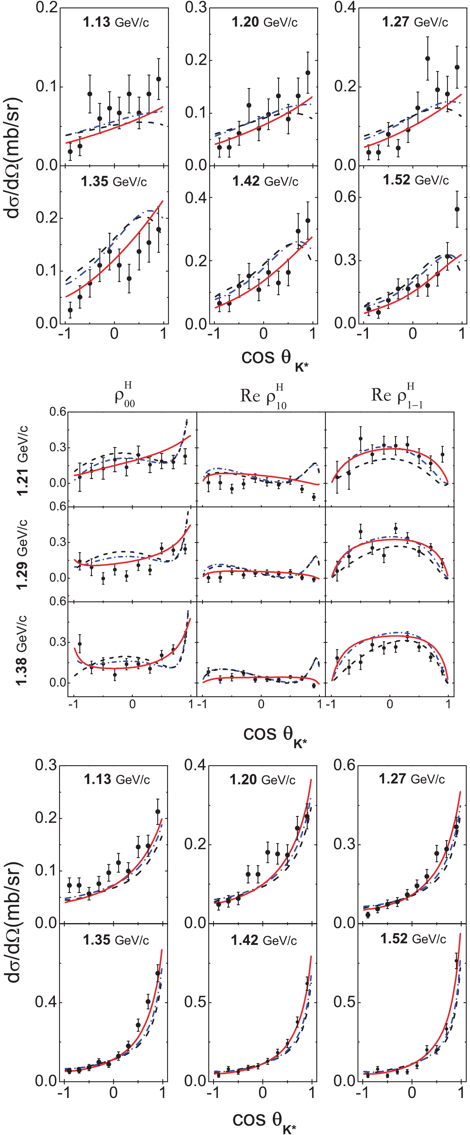Figure2. (color online) Fit results for the angular distributions (top) and SDMEs (middle) of $K^*$ in the reaction $K^+ p \to p K^{*+}(\to K^0\pi^+)$, and the angular distributions of $K^*$ in the reaction $K^+ n \to pK^{*0}( \to K^+ \pi^-)$(bottom), in the center-of-mass frame for various beam momenta. The dashed (black), dash-dotted (blue) and solid (red) lines correspond to the results of Model I, Model IIA and Model IIB, respectively. The angular distributions of $K^*$ were calculated with the amplitudes listed in Eqs. (9)-(11). $\theta_{K^*}$ is defined as $\pi-\theta_p$ with $\theta_p$ the scattering angle of the final proton in the center-of-mass frame. The experimental data are from Refs. [31, 32].

To illustrate why the present model cannot reproduce the data very well, we study the contribution of the individual Feynman diagrams. In Fig. 3 and Fig. 4, we plot the angular distributions and SDMEs of $ K^* $ in the $ K^+p\to K^{*+} p $ reaction at $ p_K = 1.2 $ GeV, where the individual contributions are shown. It can be seen that the forward enhancement in the angular distributions favors the $ \pi $ exchange, since such an enhancement cannot be provided by the vector meson exchange. On the contrary, the SDME data clearly favor the $ \omega $ exchange and exclude the possibility that the $ \pi $ exchange dominates the reaction. In fact, based on this finding the authors of Ref. [14] argued that the vector meson exchange should be dominant. Nevertheless, this argument could result in a poor prediction of the angular distributions at the forward angles. In our results (black dashed lines in Fig. 2), the poor description of the angular distributions and the Re$ \rho_{10} $ data at forward angles illustrates the limitations of the present model. On the one hand, SDME data result in a relatively small value of the cutoff of the $ K^*K\pi $ vertex obtained in the fit, which suppresses the $ \pi $ exchange and leads to a poor prediction of the angular distributions at the forward angles. On the other hand, problems in reproducing the Re$ \rho_{10} $ data at forward angles show that the $ \pi $ exchange is still too large. Such problems originate from the conflicting demands of the angular distribution and SDME data. It seems that considering only the $ \pi $, $ \rho $ and $ \omega $ exchange, the angular distribution and SDME data cannot be simultaneously well described. As a byproduct, the results shown in Fig. 4 also explain why the interference terms between the $ \pi $ and $ \rho $(or $ \omega $) exchange vanish. This is most clearly illustrated by the result for $ \rho_{00} $ measured in the Gottfried-Jackson frame. For the $ \pi $ exchange, the resultant $ \rho_{00}^{ { {{G-J}}}} $ is 1, while for the vector meson exchange $ \rho_{00}^{ { {{G-J}}}} $ is 0. This means that $ K^* $ induced by the $ \pi $ and $ \rho $($ \omega $) exchanges are in the orthogonal spin states. Thus, there are no interference terms between them.
Figure3. (color online) Contribution of the individual meson exchange diagrams in the $ K^+p\to pK^{*+}(\to\pi^+K^0) $ reaction for $ p_{K^+} = 1.2 $ GeV in Model I.

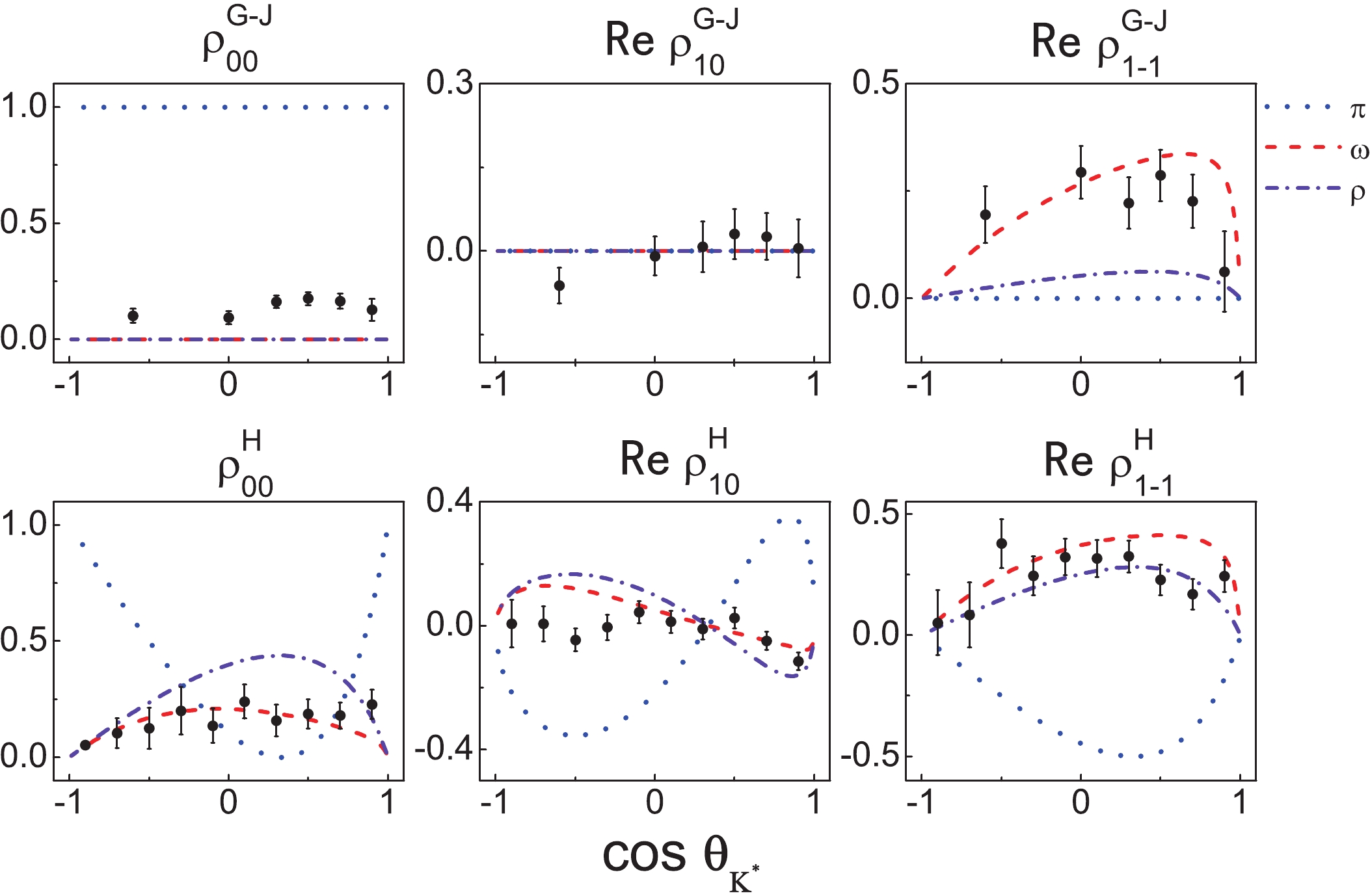Figure4. (color online) Density matrix elements induced by the individual diagrams for p_K⁺ = 1.2 GeV and the experimental data [31].

2 -->

3.2.Model II

In Model I, it was shown that by only considering the $ \pi $, $ \rho $ and $ \omega $ exchange, one cannot give a satisfactory description of the experimental data. In the following, we include the contributions of the $ a_1 $, $ \Lambda $ and $ \Sigma $ exchange diagrams.
We include the contribution of these new diagrams in two steps to show their effect on improving the model. First, we only include the hyperon exchange diagrams (Model IIA). In this case, to evaluate the amplitudes, the coupling constants and cutoff parameters of the $ KNY $ and $ K^*NY $ vertices need to be determined. The coupling constants are relatively well known from the $ KN $ scattering, or some other strange production processes [22, 27], and we use the values from literature as listed in Table 2. Since we are dealing with the u-channel hyperon exchange diagrams, the cutoff parameters are poorly known. Therefore, we treat the cutoff parameters in the $ K^*NY $ vertex, $ \Lambda_\Lambda $ and $ \Lambda_\Sigma $, as free parameters. We now have 9 free parameters in total. The fit parameters are shown in Table 4 and the corresponding results are shown in Fig. 2 by the blue dash-dotted line. The obtained $ \chi^2/dof $ for this fit is 4.32, which shows that with five more fit parameters the improvement is rather limited. An explicit study of the magnitude of the hyperon exchange shows that their contribution is small (as shown in Fig. 5), which means that the hyperon exchange diagrams play only a minor role in this reaction.

parameter	value	parameter/GeV	value
$ \phi_\pi $	1.18±0.16	$ \Lambda_\Lambda $	0.65±0.01
$ \phi_\rho $	0.56±0.22	$ \Lambda_\Sigma $/GeV	2.50±0.13
$ \phi_\Lambda $	3.20±0.14	$ \Lambda_\omega^* $	1.69±0.07
$ \phi_\Sigma $	5.10±0.12	$ \Lambda_\pi^* $	0.52±0.01
		$ \Lambda_\rho^* $	1.11±0.03

Table4.Fit parameters obtained with Model IIA ($ \chi^2/dof = 4.32 $).

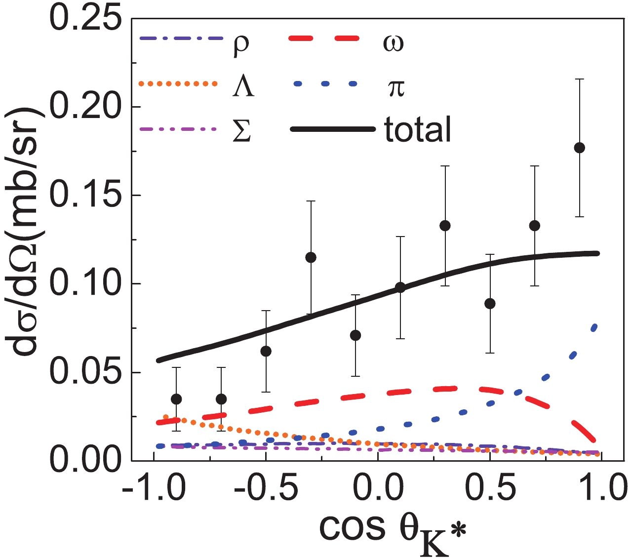Figure5. (color online) Contribution of the individual diagrams in the $ K^+ p \to pK^{*+}(\to \pi^+K^0) $ reaction for $ p_{K^+} = 1.2 $ GeV in Model IIA.

As a next step, we include the contribution of the $ a_1 $ exchange diagram (Model IIB). The Lagrangians and the coupling constants for the $ a_1KK^* $ and $ a_1NN $ vertices are discussed in the Appendix. As noted in the Introduction, there are in fact some other axial-vector meson exchanges that may contribute to this reaction. However, due to the poor knowledge of the relevant couplings, we do not consider them explicitly and assume that their contribution is partly absorbed in the $ a_1 $ exchange amplitude. The number of free parameters is 13 in this fit. The best fit parameters are shown in Table 5 and the corresponding results for the observables are shown in Fig. 2 by the red solid line. The obtained $ \chi^2/dof $ is 1.98, which shows that the contribution of the $ a_1 $ exchange significantly improves the fit results. The improvements occur both in the angular distributions and SDMEs. We have also checked that the u-channel diagrams are not important for this fit. If we turn off their contribution, the $ \chi^2/dof $ only slightly increases. However, the relative phases among the amplitudes are important for describing the data. In fact, we have fixed the relative phases according to the SU(3) relations and found that $ \chi^2/dof $ significantly increases^②.

parameter	value	parameter	value
$ \phi_\pi $	2.06±0.19	$ \Lambda_{a_1} $/GeV	2.04±0.08
$ \phi_\rho $	2.79±0.14	$ \Lambda_\omega^* $/GeV	1.48±0.09
$ \phi_\Lambda $	2.44±0.19	$ \Lambda^*_\pi $/GeV	0.55±0.04
$ \phi_\Sigma $	2.05±0.40	$ \Lambda^*_\rho $/GeV	1.04±0.05
$ \phi_{a_1} $	3.86±0.15	$ \Lambda_\Lambda $/GeV	0.58±0.02
$ \theta_{a_1} $	3.59±0.76	$ \Lambda_\Sigma $/GeV	2.50±0.11
$ g_{a_1KK^*} $	18.26±2.23

Table5.Fit parameters obtained with Model IIB ($ \chi^2/dof = 1.98 $).

The individual contributions in Model IIB are shown in Fig. 6. It is found that in this model the $ \pi $, $ \omega $ and $ a_1 $ exchange plays an important role. The strength of the $ a_1 $ exchange is comparable to that of $ \pi $ and $ \omega $. The significant contribution of $ a_1 $ is due to the large fitted coupling constant $ g_{a_1KK^*} $ and mixing angle $ \theta_{a_1} $. The present knowledge of these two parameters is rather poor. As discussed in the Appendix, to constrain these two parameters, we also take into account in the fit the experimental partial decay width of $ a_1\to KK^* $. With the fitted coupling constant, the obtained partial width $ \Gamma_{a_1KK^*} $ is 79.92 MeV, and the corresponding branching ratio is 18.80% using $ \Gamma_{a_1} = 425 $ MeV [16]. The fit result for the decay branching ratio is larger than the experimental value (2.2%-15%) [16], indicating that the experimental data favor a large contribution from the axial-vector meson exchange. The large partial decay width of $ a_1 $ obtained in the fit and the value of $ \chi^2/dof $ show that there is room for improvement of the model. One possibility is that some other axial-vector meson is also important, but is ignored in the present model. Possible contributions may come from $ f_1(1285) $, $ h_1 $, $ b_1 $ or some other higher mass mesons whose contributions are difficult to include due to the lack of knowledge of their couplings to $ NN $ and $ KK^* $. It should also be noted that to identify the $ a_1KK^* $ coupling or the partial decay width of $ a_1 $ in the $ KK^* $ channel, one should also take into account the uncertainties of $ g_{a_1NN} $. If a larger value of $ g_{NNa_1} $ is used, the obtained $ \Gamma_{a_1\to KK^*} $ can be reduced. The current knowledge of this coupling constant comes mainly from the analysis of the axial-vector form factor of the nucleon based on the axial-vector meson dominance model [33]. In these studies, the uncertainties of the extracted $ g_{a_1NN} $ are not well controlled [17, 33, 34]. Therefore, it is still not possible to draw a decisive conclusion about $ g_{a_1KK^*} $. However, the significant improvement of $ \chi^2/dof $ compared to Model I shows that the axial-vector meson exchange may be important and deserves further studies.
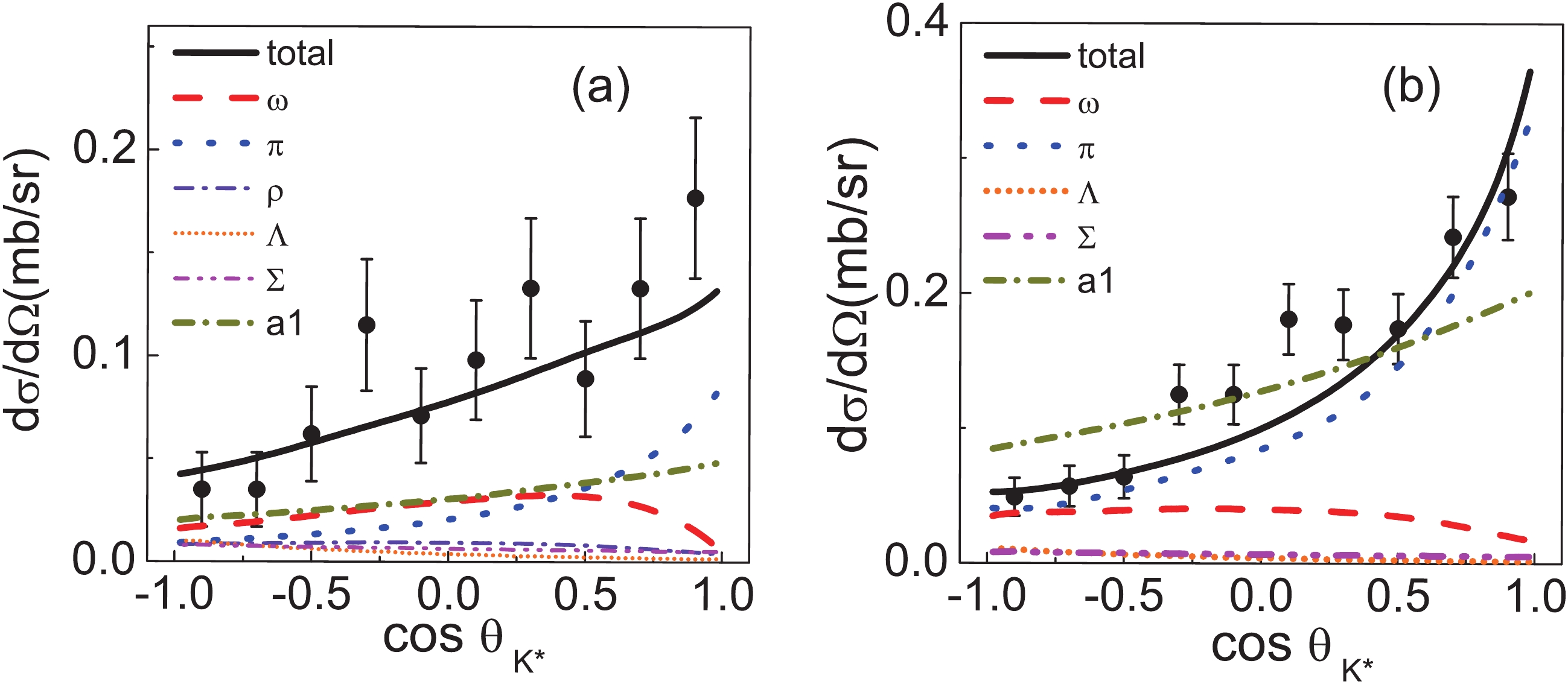Figure6. (color online) Contribution of the individual diagrams in the reactions $ K^+ p \to pK^{*+}( \to K^0 \pi^+) $(a) and $ K^+ n \to pK^{*0}( \to K^+ \pi^-) $(b) for $ p_{K^+} = 1.2 $ GeV based on Model IIB.

It is interesting to note that compared to $ K^+p \to p K^{*+} $, all models give a fairly good description of the angular distribution data for the $ K^+n \to p K^{*0} $ reaction. It is hence important to check whether the models also describe well the SDME data of this reaction. Unfortunately, such a comparison is still not possible due to the absence of data, indicating the need for new and updated data for the relevant reactions. One candidate reaction is $ K_{\rm L} N \to K^{*} N $. In fact, this has already been suggested using the secondary $ K_{\rm L} $ beam at JLab [10]. The new data for the $ K_{\rm L}N \to K^*N $ reaction could verify our models and help to better understand the reaction mechanism. We give the predictions of the angular distributions and SDMEs for the $ K_{\rm L} p \to K^{*0} p $ reaction in Fig. 7. The fact that the models result in distinct predictions indicates that they can be distinguished once the data for the $ K_{\rm L}N \to K^*N $ reaction are available.
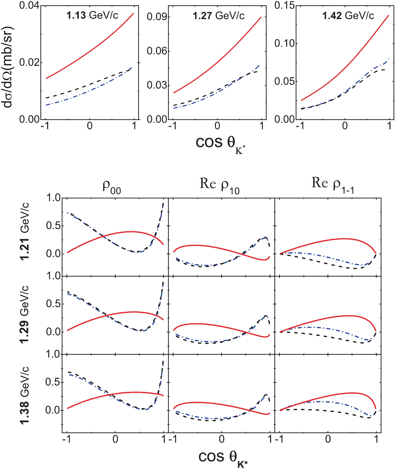Figure7. (color online) Predictions of the angular distributions and SDMEs (Helicity frame) of $ K^* $ in the $ K_{\rm L} p \to K^{*0} p $ reaction in the center-of-mass frame for various beam momenta, based on Model I (black dashed line), Model IIA (blue dash-dotted line) and Model IIB (red solid line).

In the present work, we investigated the $ K^* $ production in the $ KN\to K \pi N $ reaction using the effective Lagrangian approach. We calculated the contributions of $ \pi $, $ \rho $, $ \omega $, hyperons and axial-vector meson exchange. The available experimental data, such as the angular distributions and spin density matrix elements were analyzed. It was found that Model IIB is favored by the existing experimental data, in which the pseudoscalar meson ($ \pi $), vector meson ($ \omega $) and axial-vector meson ($ a_1 $) exchanges are important for understanding of this reaction. In order to identify the role of the axial-vector meson exchange, measurements of $ K_{\rm L} p\to K^{*0} p $ would be helpful. Model predictions for this reaction were also presented for a future comparison.

In this Appendix, we present the Lagrangains and coupling constants for the $ a_1NN $ and $ a_1KK^* $ vertices. For the $ a_1NN $ vertex, we use the following Lagrangian [17],

$\tag{A1} \begin{array}{l} {\cal L}_{NNa_1} = g_{NNa_1}\bar{N}\gamma_\mu \gamma_5 N a_1^\mu . \end{array} $

The coupling constant $ g_{NNa_1} $ is difficult to determine directly. In practice, it can be evaluated from the nucleon axial-vector coupling constant based on the axial-vector meson dominance model. The uncertainty of this method comes from the model itself and from the ratio of $ g_A/g_V $ used in the model. For example, one gets $ g_{NNa_1} = 6.70\pm 1.0 $ [17, 33] and $ g_{NNa_1} = 7.49\pm 1.0 $ [34] by using different values of $ g_A/g_V $. Bearing the uncertainties in mind, we use $ g_{NNa_1} = 6.70 $ in this work.
The Lagrangian for the $ a_1KK^* $ vertex is [35],

$\tag{A2} \begin{array}{l} {\cal L}_{a_1KK^*} = \frac{g_{a_1KK^*}}{\sqrt{2}}({\cal L}_1 \cos\theta_{a_1}+{\cal L}_2 \sin\theta_{a_1}) , \end{array} $

with

$ \begin{array}{l} {\cal L}_1 = \partial^\nu \bar{K} a_1^\mu K^*_{\mu\nu}+h.c.,\\ {\cal L}_2 = \bar{K} \partial^\mu a_1^\nu K^*_{\mu\nu}+h.c., \end{array} $

and $ K^*_{\mu\nu} = \partial_\mu K^*_\nu-\partial_\nu K^*_\mu $. With the Lagrangians given above, the $ a_1 $ exchange amplitude can be expressed as

$\tag{A3} \begin{split}{{\cal A}_{{a_1}}} =&{ - \sqrt 2 {G_V}{g_{{a_1}NN}}{g_{{a_1}K{K^*}}}\frac{{ - {g_{\mu \nu }} + \frac{{{p_{{K^*},\mu }}{p_{{K^*},\nu }}}}{{p_{{K^*}}^2}}}}{{p_{{K^*}}^2 - m_{{K^*}}^2 + {\rm i}{m_{{K^*}}}\Gamma }}}\\&\times{\left[ {\left( {p_{{K^*}}^\alpha p_K^\nu {\rm cos}\theta + p_{{K^*}}^\alpha p_{{a_1}}^\nu {\rm sin}\theta } \right)\frac{{ - {g_{\alpha \beta }} + \frac{{{p_{{a_1},\alpha }}{p_{{a_1},\beta }}}}{{p_{{a_1}}^2}}}}{{p_{{a_1}}^2 - m_{{a_1}}^2}}} \right.}\\&{\left. { {\left. { - ({p_{{K^*}}} \cdot {p_K}{\rm cos}\theta + {p_{{K^*}}} \cdot {p_{{a_1}}}{\rm sin}\theta } \right)\frac{{ - {g_{\nu \beta }} + \frac{{{p_{{a_1},\nu }}{p_{{a_1},\beta }}}}{{p_{{a_1}}^2}}}}{{p_{{a_1}}^2 - m_{{a_1}}^2}}} } \right]}\\&\times{( - p_{{\pi ^ + }}^\mu + p_{{K^0}}^\mu ){\gamma _\beta }{\gamma _5}.}\end{split}$

In previous studies, the coupling constant $ g_{a_1KK^*} $ and the mixing angle $ \theta_{a_1} $ are rarely studied. In practice, one can extract the coupling constant from the partial decay width. For the $ a_1 \to KK^* $ process, there are indeed some experimental values [36-38]. However, one cannot determine both of these parameters with one input. In this work, we choose to set them as free parameters and obtain them from the simultaneous fit of the data for the reactions $ K^+ p\to K^{*+} p $ and $ K^+ n\to K^{*0} p $ and their partial widths.
Since $ a_1 $ lies below the $ KK^* $ threshold, the decay is due to its width. The partial decay width $ \Gamma_{a_1\to KK^*} $ can be calculated as [39]

$\tag{A4} \begin{split} \Gamma_{a_1\to KK^*} =& \frac{1} {\pi^2}\int {\rm d}s_{ { {{a_1}}}} {\rm d}s_{ { {{K^*}}}} \\ &\times {\rm Im}\left(\frac{1}{s_{ { {{K^*}}}}-M_{ { {{K^*}}}}^2+{\rm i}M_{ { {{K^*}}}}\Gamma_{K^*}}\right) {\rm Im}\left(\frac{1}{s_{ { {{a_1}}}}-M_{ { {{a_1}}}}^2+{\rm i}M_{ { {{a_1}}}}\Gamma_{ { {{a_1}}}}}\right) \\ &\times\Gamma_{ { {{a_1KK^*}}}}(\sqrt{s_{ { {{a_1}}}}},\sqrt{s_{ { {{K^*}}}}}) \Theta(\sqrt{s_{ { {{a_1}}}}}-\sqrt{s_{ { {{K^*}}}}}-M_{ { {{K}}}}), \end{split} $

where

$\tag{A5} \begin{array}{l} \Gamma_{a_1KK^*} = \frac{q}{12\pi M_A^2}\sum|M_{a_1\rightarrow KK^*}|^2 \end{array} $

and $ M_{a_1\rightarrow KK^*} $ is the decay amplitude. To make the integral converge, it is necessary to consider the form factors. We follow Ref. [40] and add

$\tag{A6} \begin{array}{l}\left(\frac{\Lambda_{a_1}^2}{\Lambda_{a_1}^2+|s_A-m_{a_1}^2|}\right)^2\cdot \left(\frac{\Lambda_{K^*}^2}{\Lambda_{K^*}^2+|s_V-m_{K^*}^2|}\right) \end{array} $

in the amplitude. Note that we use a dipole form factor for $ a_1 $ since the $ a_1KK^* $ coupling involves both the S-wave and D-wave.
To obtain the results presented in the text, we use $ \Lambda_{a_1} = \Lambda_{K^*} = 1.0 $ GeV as in Ref. [40]. The partial decay width of $ a_1\rightarrow KK^* $ obtained in Model IIB is 79.92 MeV and the corresponding decay branching ratio is 18.80%. Note that we have also tried in the fit the values of 1.5 and 2.0 GeV for $ \Lambda_{a_1} $ and $ \Lambda_{K^*} $. The corresponding values for the partial decay width are 106.35 and 121.81 MeV, respectively, with a worse $ \chi^2/dof $.