Jingyi Chao ^,
,

Corresponding author: Jingyi Chao, jychao@impcas.ac.cn

Institute of Modern Physics, Chinese Academy of Sciences, Lanzhou 730000, China
Received Date:2019-11-15
Available Online:2020-03-01
Abstract:We study the two-color QCD matter with two fundamental quark flavors using the chiral perturbation theory and the Nambu-Jona-Lasinio (NJL) model. The effective Lagrangian is derived in terms of mesons and baryons, i.e. diquarks. The low lying excitations lie in the extended $ {SU}(4)$ flavor symmetry space. We compute the leading order terms of the Lagrangian as a function of the baryon and axial isospin densities. After numerically solving the gap equations in the two-color NJL model, the phase diagram is obtained in the $\mu-\nu_{5}$ plane.

HTML

--> --> -->

The color superconductivity in Quantum Chromodynamics (QCD) matter at high baryon density, such as in the core of a neutron star, has been extensively studied, see e.g. [1] for a review and references therein. Several studies have shown that the consequences of the large superconducting gap should be observed in astrophysics or heavy-ion collision experiments. However, this has not been definitively confirmed by the first principles calculations due to the sign problem in the lattice Monte Carlo simulations in dense QCD matter [2, 3]. It has therefore been proposed to understand the quark matter at finite baryon density in simpler QCD-like theories. For example, in the $ N_{c} = 2 $ gauge theory, the fermion determinant is guaranteed to be real for nonzero chemical potential due to the additional anti-unitary symmetry, which allows a discrete evaluation of the fundamental and adjoint quarks [4-15]. On the other hand, the flavor space could be extended from the usual $ {SU}(N_{f}) $ to the larger $ {SU}(2N_{f}) $ [4, 7, 8]. The two-color QCD framework ($ {\rm QC_{2}D} $) is somewhat different from the full three-color gauge theory in the sense that the baryons are bosons rather than fermions. Nevertheless, this approach sheds light on the mechanism of phase transitions, the formation of diquark condensate and critical phenomena, in realistic QCD matter.
The investigation of the QCD phase diagram for finite baryon and nonzero isospin densities has attracted considerable attention [8, 16-19]. The main reason is that the dense hadronic matter is isotopically asymmetric in heavy-ion collision experiments [20, 21]. The interior of compact stars is also expected to be isospin asymmetric [22]. A large class of effective theories, such as the chiral perturbation theory [8, 16], the Nambu–Jona-Lasinio (NJL) type models [23-27], linear sigma models [28], the Polyakov-Quark-Meson models [29, 30], the Dyson-Schwinger equations [31] and functional renormalization group methods [32, 33], have been used to explore the alignment of the vacuum expectation value (VEV) and the matter phase structure.
The study of QCD matter in external electromagnetic (EM) environment [34-40] has become of interest since the charge separation along the magnetic field was observed in non-central heavy-ion collisions at the Relativistic Heavy Ion Collider (RHIC) [41]. A background EM field exists in various physical systems, such as in compact stars [42], the early Universe [43] and at RHIC and the Large Hadron Collider [41, 44, 45]. The EM field excites charged particles in both the hadronic and quark-gluon plasma (QGP) phases, offering a unique opportunity for exploring the QCD vacuum structure and the thermodynamics of strongly interacting matter. Several approaches have been used to understand the phenomena of magnetic catalysis at low temperature, and of the inverse magnetic catalysis near $ T_{c} $ in magnetized quark matter [46-50]. It was suggested that the QCD vacuum becomes a superconductor due to charged $ \rho $ condensation [51-55]. Recently, the EM chiral anomaly has triggered new interest in investigating the QCD phase diagram in a (anti)parallel EM environment, i.e. in (anti)parallel electric and magnetic fields [56-58]. In [56], the authors found that the pion superfluidity is energetically favored when the strength of EM fields is increased. Indeed, the chiral anomaly is closely linked to various quantum phenomena in EM fields, such as the chiral magnetic effect [59], chiral magnetic waves [60] and chiral electrodynamics [61].
As a consequence, there is a good reason to study the behavior of diquarks in electromagnetized dense baryon matter, as the EM field acts on all charged collective modes, and the diquarks can be treated as elementary states of QCD matter at high baryon density [7, 9]. If only the QCD interactions are considered, the axial isospin current is anomaly free. The EM chiral anomaly arises when quarks couple to the electromagnetic field. The corresponding current is given by

$ \partial_{\mu}j_{5}^{\,\mu 3} = -\frac{e^{2}}{16\pi^{2}} \varepsilon^{ \alpha \beta\mu\nu}F_{ \alpha \beta}F_{\mu\nu}\cdot {\rm tr} \left[\tau_{3}Q^{2} \right], $

(1)

where Q is the matrix of quark electric charges, $ \tau_{3} $ is the Pauli matrix in flavor space and F is the field strength. A related process is the decay of a neutral pion into two photons [62-64]. In order to qualitatively study the charge asymmetry in a strong EM field, we introduce an axial isospin chemical potential $ \nu_{5} $, and $ \nu_{5}\bar{\psi} \gamma_{0} \gamma_{5}\tau_{3}\psi $ is included in the quark sector of the Lagrangian [65, 66]. A similar fermionic part of the Lagrangian, in the parameter space of the isospin chemical potential instead of $ \nu_{5} $, was studied in [67] with twisted mass Wilson fermions.
In order to determine the properties of diquarks in EM fields, we compute in this work the QCD phase diagram in the plane of baryon and axial isospin chemical potentials in two-color QCD, which consists of the two-color gauge group with two Dirac flavors in the fundamental representation. This model dynamically generates quasi-particles in terms of sigmas, pions and baryons (diquarks). The details of the model are given in Sec. 2. In Sec. 3, we derive the underlying effective Lagrangian. Using the static low-energy effective $ {\cal L} $, we identify the breaking patterns of the global symmetries. The NJL model is solved numerically and the results are shown in Sec. 4. The conclusions are presented in the final section.

We start with the following NJL Lagrangian for the $ {\rm QC_{2}D} $ model, where the effective four-fermion interactions are included in a gluon inspired manner; more details can be found in [11]. The Lagrangian reads

$\begin{split} {\cal L}_{ {\rm NJL}} = &\bar{\psi} \left( {\rm i} \gamma^{\mu} \partial_{\mu}+\mu \gamma_{0}+\nu_{5} \gamma_{0} \gamma_{5}\tau_{3}-m_{0} \right)\psi\\&+ {\cal L}_{\bar{q}q}+ {\cal L}_{qq}+({\rm{color}} \;{\rm{triplet}} \;{\rm{terms}}), \end{split} $

(2)

$ {\cal L}_{\bar{q}q} = \frac{G}{2} \left[(\bar{\psi}\psi)^2+(\bar{\psi} {\rm i} \gamma_{5}\vec{\tau}\psi)^2 \right], $

(3)

$\begin{split} {\cal L}_{qq} =& \frac{H}{2}(\bar{\psi} {\rm i} \gamma_{5}\tau_{2}t_{2}C\bar{\psi}^{T})({\psi}^{T}C {\rm i} \gamma_{5}\tau_{2}t_{2}{\psi})\\&-\frac{H}{4}(\bar{\psi} \gamma_{3}\tau_{1}t_{2}C\bar{\psi}^{T})({\psi}^{T}C \gamma_{3}\tau_{1}t_{2}{\psi}), \end{split}$

(4)

where $ C = {\rm i} \gamma_{0} \gamma_{2} $ is the charge conjugation operator, $ m_{0} $ is the current quark mass, and $ \tau_{i} $ and $ t_{i} $ are the Pauli matrices in flavor and color spaces, respectively. $ \tau_{2}, t_{2} $ are the antisymmetric matrices. The two coupling constants G and H are connected by the Fierz transformation in color space. In particular, $ G = H $ for $ N_{c} = 2 $.
Since $ \nu_{5} = \mu_{L}^{u}-\mu_{R}^{u} = \mu_{R}^{d}-\mu_{L}^{d} $, where the left-handed u quark is on the same Fermi surface as the right-handed d quark, while the baryon density of the right-handed u quark is equal to the left-handed d quark, the corresponding LR bound states composed of two quarks on equal Fermi surfaces are $ \psi_{L}^{u}\psi_{R}^{d}\pm\psi_{R}^{u}\psi_{L}^{d} $. Focusing on the anti-symmetric color sector, where the attraction is stronger, the Dirac structure of the total antisymmetric LR diquark $ \psi_{L}^{u}\psi_{R}^{d}-\psi_{R}^{u}\psi_{L}^{d} $ is in the repulsive $ (C \gamma_{0} \gamma_{5}) $ channel with zero spin and isospin, which cannot form a bound particle. On the other hand, the flavor symmetric state, $ \psi_{L}^{u}\psi_{R}^{d}+\psi_{R}^{u}\psi_{L}^{d} $ is attractive with Dirac operator $ (C \gamma_{3}) $. Symmetric flavor diquark pairing patterns have been explored in the same- or one-flavor color superconductors [68-74]. It was suggested that, except for the most attractive scalar diquark ($ C \gamma_{5} $), the axial spin diquark pairs are formed. Hence, for finite $ \nu_{5} $, the system prefers the polar phase ($ s = 1 $, $ s_{z} = 0 $) for symmetric spin, and the $ \tau_{1} $ channel for symmetric flavor, to satisfy the Pauli exclusion principle.
In [56, 75], the authors showed that the QCD vacuum makes a chiral rotation from the scalar $ \sigma $ condensate to the pseudo-scalar $ \pi_{i} $ condensates as a result of the EM chiral anomaly. Therefore, based on these considerations, we apply in this work the Hubbard-Stratonovich transformation and introduce three kinds of auxiliary meson and diquark fields: $ \pi_{3} = -\frac{G}{2}\left\langle {\bar{\psi} {\rm i} \gamma_{5}\tau_{3}\psi} \right\rangle $ represents the neutral pseudo-scalar, $ \Delta = -\frac{H}{2}\left\langle {\psi^{T} {\rm i} \gamma_{5}\tau_{2}t_{2}C\psi} \right\rangle $ and $ \Delta^{*} = -\frac{H}{2} $$\left\langle {\bar{\psi} {\rm i} \gamma_{5}\tau_{2}t_{2}C\bar{\psi}^{T}} \right\rangle $ denote the complex scalar diqurks, and $ d = -\frac{H}{4}\left\langle {\psi^{T} \gamma_{3}\tau_{1}t_{2}C\psi} \right\rangle $ and $ d^{*} = -\frac{H}{4}\left\langle {\bar{\psi} \gamma_{3}\tau_{1}t_{2}C\bar{\psi}^{T}} \right\rangle $ are the complex axial vector diquarks. In terms of the Nambu-Gorkov bispinors

$ \psi = \frac{1}{{\sqrt 2 }}\left( {\begin{array}{*{20}{c}} q\\ {C{{\bar q}^T}} \end{array}} \right),\;\;\;\bar \psi = \frac{1}{{\sqrt 2 }}\left( {\bar q,{q^T}C} \right), $

(5)

the effective thermodynamical potential is written as

$ \Omega_{\rm{eff}} = \frac{1}{2}\bar{\psi} {\cal S}^{-1} \left(p;\pi_{3}, \Delta,d \right)\psi-\frac{\pi_{3}^2+| \Delta|^2+|d|^2}{4G}. $

(6)

Here, the inverse propagator of the fermion is

$ {S^{ - 1}}(p) = \left( {\begin{array}{*{20}{c}}\!\!\!\! {{\not\!\! p} \!-\! M \!+ \!{\gamma _0}\mu + {\gamma _0}{\gamma _5}{\tau _3}{\nu _5}}&{\tilde \Delta }\\ { - {{\tilde \Delta }^\dagger }}&\!\!\!\!{{\not\!\! p}\! - \!{M^T}\! - \!{\gamma _0}\mu \!+\! {\gamma _0}{\gamma _5}{\tau _3}{\nu _5}} \end{array}}\!\!\!\! \right), $

(7)

where $ M = \left(m_{0}- \sigma \right)\tau_{0}- {\rm i} \gamma_{5}\tau_{3}\pi_{3} $ and $ \tilde{ \Delta} = \gamma_{5}\tau_{2} \Delta+ \gamma_{3}\tau_{1}d $. The color index has been omitted since it becomes trivial in the calculations below.

In this section, we briefly explain the behavior of $ \pi_{3} $, $ \Delta $ and d given the external conditions in the framework of the chiral perturbation theory.
The fundamental representation of the group $ {SU}(2) $ is pseudo-real and is isomorphic to its complex conjugate representation with the isometry given by $ S = {\rm i} \sigma_{2} $ [4, 7, 8]. In other words, charge conjugation of the gauge fields when $ N_{c} = 2 $ is equivalent to a constant gauge transformation of S. Therefore, left- and right-handed spinors get interchanged under the anti-unitary symmetry $ T = CSK $, where C is the charge conjugation matrix in spinor space and K is complex conjugation. One may write the spinors as

$ \Psi = \left( {\begin{array}{*{20}{c}} {{\psi _L}}\\ {{{\tilde \psi }_R}} \end{array}} \right),\;\;\;{\Psi ^\dagger } = \left( {\psi _L^\dagger ,\tilde \psi _R^\dagger } \right),$

(8)

where $ \tilde{\psi}_{R} = T\psi_{R} = - {\rm i} \sigma_{2}S\psi_{R}^{*} $ and $ - {\rm i} \sigma_{2} $ is the C matrix for the right spinor. This gauge theory has a larger flavor symmetry $ {SU}(2N_{f}) $. In the extended flavor space, $ \Psi $ manifests its flavor symmetry and chiral component at the same time, establishing a connection between quarks and anti-quarks [4, 7, 8]. As a consequence, color singlet baryons are composed of two quarks, and scalar diquarks become degenerate with pseudo-mesons (pions).
Using the above expression, the standard kinetic part of the Euclidean $ {\rm QC_{2 }D} $ Lagrangian can be written as [14]

$ {\cal L}_{ {\rm kin}} = \Psi^{\dagger} {\rm i} \sigma^{\mu}D_{\mu}\Psi, $

(9)

where $ \sigma^{\mu} $ is the Hermitian gamma matrix $ \sigma^{\mu} = (- {\rm i},\vec{ \sigma}) $, and $ D_{\mu} $ is the covariant derivative $ D_{\mu} = \partial_{\mu}+ {\rm i} A_{\mu}^{a}T_{a} $. The coupling constant is absorbed in the gauge fields. Similarly, the quark mass term becomes [14]

$ {\cal L}_{ {\rm mass}} = \frac{m_{0}}{2} \left(\Psi^{T} {\rm i} \sigma_{2}SE_{4}\Psi-\Psi^{*T} {\rm i} \sigma_{2}SE_{4}\Psi^{*} \right), $

(10)

where the symplectic matrix $ E_4 $ is

$ {E_4} = \left( {\begin{array}{*{20}{c}} 0&{{\tau _0}}\\ { - {\tau _0}}&0 \end{array}} \right).$

(11)

The group $ {SU}(4) $ has $ 15 $ generators. In the block representation, the $ 10 $ symmetric elements are [76, 77]

$ S_{a} = \frac{1}{2\sqrt{2}} \left({\begin{array}{*{20}{c}} \tau_{a}&0\\ 0&-\tau_{a}^{T} \end{array}} \right),\quad {\rm for }\; a = 0,1,2,3; $

(12)

$ S_{a} = \frac{1}{2\sqrt{2}} \left({\begin{array}{*{20}{c}} 0& B_{a}\\ B_{a}^{\dagger}&0 \end{array}} \right),\quad {\rm for }\; a = 4,\cdots,9\ , $

(13)

with $ B_{(4,5)} = {\rm i}^{(0,1)}\tau_{0}, B_{(6,7)} = {\rm i}^{(0,1)}\tau_{3} $ and $ B_{(8,9)} = {\rm i}^{(0,1)}\tau_{1} $. The remaining five anti-symmetric generators are:

$ X_{i} = \frac{1}{2\sqrt{2}} \left({\begin{array}{*{20}{c}} \tau_{i}&0\\ 0&\tau_{i}^{T} \end{array}} \right),\quad {\rm for }\; i = 1,2,3; $

(14)

$ X_{i} = \frac{1}{2\sqrt{2}} \left({\begin{array}{*{20}{c}} 0& D_{i}\\ D_{i}^{\dagger}&0 \end{array}} \right),\quad {\rm for }\; i = 4,5 \ , $

(15)

with $ D_{(4,5)} = {\rm i}^{(0,1)}\tau_{2} $.
$ {SU}(4) $ explicitly (dynamically) reduces to the symplectic group $ {Sp}(2) $ as a result of the current (constituent) quark mass. The generators of $ {Sp}(2) $ obey the relation $ S_{a}^{T}E_{4}+E_{4}S_{a} = 0 $, with the mass operator $ E_{4} $, which clearly indicates that the bare mass term is only invariant under the subgroup of $ {Sp}(2) $. Thus, $ E_{4} $ and $ X_{i} $, the elements of the coset subgroup $ {SU}(4)/ {Sp}(2) $, form a six-dimensional vector of chiral order parameters under the quark bilinears ($ \Psi^{T}\vec{\phi}\,\Psi+{\rm h.c.} $). Five almost Goldstone bosons $ \vec{\pi},\, \Delta $ and $ \Delta^{*} $ are created. Note that here $ \vec{\phi} = (E_{4}, {i} E_{4}X_{i},X_{j}) $ for $ i = 1,2,3 $ and $ j = 4,5 $, where $ E_4 $ is the generator of scalar meson $ \sigma $, $ {i} E_{4}X_{(1,2,3)} $ represents the pseudo-scalar triplet pions $ \vec{\pi} $, and $ X_{(4,5)} $ denote the scalar diquark and anti-diquark $ \Delta $ and $ \Delta^{*} $.
Employing the above representation, the conventional baryon Lagrangian term $ \mu\bar{\psi} \gamma_{0}\psi $ is rewritten in the $ SU(4) $ space as $ \mu\Psi^{\dagger}B_{0}\Psi $ [14], where

$ B_{0} = - \gamma_{0}E_{4} = \left({\begin{array}{*{20}{c}} \tau_{0}& 0\\ 0& -\tau_{0} \end{array}} \right). $

(16)

Similarly, the isospin current $ \nu\,\bar{\psi} \gamma_{0}\tau_{3}\psi $ is written as $ \nu\,\Psi^{\dagger}I_{0}\Psi $ with $ I_{0} = {\rm Diag}(\tau_{3},-\tau_{3}) $. The term with axial isospin density $ \nu_{5}\bar{\psi} \gamma_{0} \gamma_{5}\tau_{3}\psi $ is expressed as $ \nu_{5}\Psi^{\dagger}I_{5}\Psi $ with $ I_{5} = \gamma_{5}I_{0} = {\rm Diag}(\tau_{3},\tau_{3}) $.
For finite isospin density, applying the gauge transformation [7, 8]

$ \Psi\to V\,\Psi, \quad V = \exp \left( {\rm i} \theta^{i}X_{i} \right)\quad {\rm for}\; X_{i}\in {SU}(4)/ { Sp}(2), $

(17)

one has $ \left[X_{i},I_{0} \right]\neq 0 $ for $ i = 1,2 $. This means, as is well known, that the isospin baryon current is embedded in the charged mesons $ \pi_{\pm} $ to compensate the gauge transformation. Replacing the derivatives by covariant derivatives, one gets the leading order terms of the Lagrangian in the chiral perturbation theory ($ \chi {\rm PT} $) [7, 8]

$ {\cal L}_{\chi {\rm PT}} = \frac{f_{\pi}^{2}}{4} {\rm Tr} \left(D_{\mu} \Sigma^{\dagger} \right) \left(D_{\mu} \Sigma \right)-c {\rm Tr}{ \left( \Sigma^{\dagger}+ \Sigma \right)}, $

(18)

where the unitary matrix $ \Sigma $ consists of the fluctuations of the symmetry breaking order parameters with respect to the extended $ SU(4) $ flavor group, and the second term is induced by the quark mass. As shown in [8], the long covariant derivatives can be written explicitly as:

$ \begin{array}{l}\;\;\; D_{\mu} \Sigma = \partial_{\mu} \Sigma+ \left(I_{\mu} \Sigma+ \Sigma I_{\mu}^{T} \right) \\ D_{\mu} \Sigma^{\dagger} = \partial_{\mu} \Sigma^{\dagger}- \left( \Sigma^{\dagger}I_{\mu}+I_{\mu}^{T} \Sigma^{\dagger} \right). \end{array} $

(19)

After expansion, two non-derivative terms appear in a linear combination of

$ {\rm Tr} \left(I_{\mu}^{T} \Sigma^{\dagger}I_{\mu} \Sigma \right), \qquad{\rm and}\qquad {\rm Tr} \left(I_{\mu}I_{\mu} \right), $

(20)

because the trace is invariant under permutation. The second term, which is constant, is discarded. Therefore, ignoring the kinetic and mass terms, to demonstrate that the chiral orientation towards the charged pions at finite isospin density are energetically favored, the remaining static Lagrangian in [8] is expressed as

$ {\cal L}_{\chi {\rm PT}} = {\cal L}_{\pi_{i}}\sim \nu^{2} {\rm Tr} \left(I_{0}^{T}\phi_{i}^{\dagger}I_{0}\phi_{i} \right) = \nu^{2}\, {{\rm{Diag}}} \left(\tau_{3}\tau_{i}^{T}\tau_{3}\tau_{i}^{T},\tau_{3}\tau_{i}\tau_{3}\tau_{i} \right), $

(21)

where $ \phi_{i} = E_{4}X_{i} $, characterizing the bilinear meson field $ \psi^{\dagger}\psi $. When the fluctuations of the vacuum expectation value of $ \Sigma $ are neglected, the above term becomes negative for $ \tau_{i} = \tau_{1,2} $, which are correlated with $ \phi_{i}\sim X_{1,2} $, indicating that the charged pion condensate is formed for $ \mu_{I}>m_{\pi}/2 $, as expected.
At finite baryon chemical potential $ \mu $, the meson fields are unaffected by the baryon current since $ \left[X_{i},B_{0} \right] = 0 $ for $ i = 1,2,3 $. Not surprisingly, the (anti-)diquark generators $ X_{4,5} $ do not commute with $ B_{0} $. The covariant requirement modifies the scalar (anti-)diquark fields and the effective Lagrangian term is [7]

$\begin{split} {\cal L}_{\chi {\rm PT}} =& {\cal L}_{ \Delta, \Delta^{*}}\sim \mu^{2} {\rm Tr} \left(B_{0}^{T}\Phi_{i}^{\dagger}B_{0}\Phi_{i} \right) \\=& -\mu^{2}\, {{\rm{Diag}}} \left(\tau_{0}t_{i}\tau_{0}t_{i}^{\dagger},\tau_{0}t_{i}^{\dagger}\tau_{0}t_{i} \right) . \end{split}$

(22)

Here, $ t_{i} = {\rm i}^{(0,1)}\tau_{2} $ because of the complex diquarks $ \Delta $ and $ \Delta^{*} $. In the conventional $ {SU}(2) $ space, they are composed of two (anti-)quarks, $ \psi^{T}\psi $.
When the axial isospin chemical potential $ \nu_{5}\neq 0 $, excluding the commuted generator $ X_{3} $ with respect to $ I_{5} $, all other antisymmetric generators appear in the covariant part of the Lagrangian to compensate the gauge transformation of the axial isospin current. The associated Lagrangian terms in mesons space are

$ \begin{split} {\cal L}_{\chi {\rm PT}} =& {\cal L}_{\pi_{i}}\sim\nu_{5}^{2} {\rm Tr} \left(I_{5}^{T}\phi_{i}^{\dagger}I_{5}\phi_{i} \right) \\=& -\nu_{5}^{2}\, {{\rm{Diag}}} \left(\tau_{3}\tau_{i}^{T}\tau_{3}\tau_{i}^{T},\tau_{3}\tau_{i}\tau_{3}\tau_{i} \right), \end{split} $

(23)

which is positive and increases the effective potential for $ \phi_{i}\sim X_{1,2} $. This is the reason why in this work $ \pi_{3} $ is chosen to characterize the meson type of the chiral condensate at finite $ \nu_{5} $.
Moreover, in the high baryon density limit, where flavor symmetric diquarks spontaneously form a condensate, the remaining $ {Sp}(2) $ group continues to break to a reduced symmetry. It is expected that $ {Sp}(2) $ reduces to $ {O}(4) $ [76, 77]. We find that $ \left[S_{a},I_{5} \right]\neq 0 $ for $ a = 1,2,8,9 $. The $ {O}(4) $ group is left due to the six commuting elements of $ S_{a} $. In addition, the number of would be Goldstone bosons increases from $ 5 $ to $ 9 $. Two of them are the flavor triplet scalar mesons $ a_{0}^{\pm} $. The other two are the axial (anti-) diquarks $ d,\,d^{*} $. As the goal of this work is to explore the region of cold high-density quark matter where the diquark paring pattern and its behavior is more interesting than mesons, the possible appearance of new meson condensates is beyond the scope of this work. The static Lagrangian term of the diquark is modified to

$\begin{split} {\cal L}_{\chi {\rm PT}} =& {\cal L}_{ \Delta,d}\sim \nu_{5}^{2} {\rm Tr} \left(I_{5}^{T}\Phi_{i}^{\dagger}I_{5}\Phi_{i} \right) \\=& \nu_{5}^{2}\, {{\rm{Diag}}} \left(\tau_{3}t_{i}\tau_{3}t_{i}^{\dagger},\tau_{3}t_{i}^{\dagger}\tau_{3}t_{i} \right) ,\end{split} $

(24)

which is negative for $ t_{i} = {i}^{(0,1)}\tau_{1,2} $. This means that $ \Phi_{i} $ are favored as $ X_{4,5} $ or $ S_{8,9} $. The former two correspond to the scalar diquark $ \Delta $ and anti-diquark $ \Delta^{*} $, $ (C \gamma_{5}\tau_{2}t_{2}) $, while the latter two are the axial vector diquark d and anti-diquark $ d^{*} $. In the two-color space, the color singlet baryon, i.e. diquark, is composed in the anti-symmetric color channel. Thus, the flavor symmetric diquarks d and $ d^{*} $ have to be symmetric in spin space, $ (C \gamma_{3}\tau_{1}t_{2}) $, to maintain the total antisymmetry [68-74]. It should be noted that the choice of the $ \tau_{1} $ flavor space is consistent with the generator of $ S_{8,9} $. In summary, we have shown that three kinds of condensates, $ \pi_{3}, \Delta\,( \Delta^{*}), d\,(d^{*}) $, appear at the leading order of the low energy effective theory for both the finite chemical and axial isospin chemical potentials.

Considering the antisymmetric color channel alone for $ N_{c} = 2 $, a diquark is either a spin-, isospin-singlet (LL or RR quark states), or a constituent of the spin-, isospin-triplets (LR quark states), whose color space does not mix with the spin direction. Note that if three colors are available, the spins can be locked to the colors in a linear manner, where $ \lambda_{A = 2,5,7} $ correlate with the spatial directions of $ (C \gamma_{i = 1,2,3}) $. An unbroken global $ {SO}(3) $ mixture remains and the gap is isotropic, which lowers the free energy as shown in [72].
We use the single Dirac component $ (C \gamma_{3}) $ to denote the spin one diquarks. In what follows, we assume that $ \Delta = \Delta^{*} $, $ d = d^{*} $ are real quantities, as is done in most works, and apply the mean-field (Hartree) approximation. It is convenient to write the Lagrangian in the Nambu-Gorkov spinors space, as was done in Sec. 2. The thermodynamical potential is derived as

$\begin{split}\Omega(T,\mu,\nu_{5}) = &\frac{T}{2V}\ln\det {\cal S}^{-1} \left( {\rm i} \omega_{n},p;\pi_{3}, \Delta,d \right)+\frac{\pi_{3}^{2}+ \Delta^{2}+d^{2}}{4G} \\ =& -T\sum_{n}\int\frac{ {\rm d}^{3}p}{(2\pi)^{3}}\frac{1}{2} {\rm Tr}\ln \left(\frac{1}{T} {\cal S}^{-1} \left( {\rm i} \omega_{n},p;\pi_{3}, \Delta,d \right) \right) \\&+\frac{\pi_{3}^{2}+ \Delta^{2}+d^{2}}{4G}, \end{split} $

(25)

where the sum is over fermionic Matsubara frequencies $ \omega_{n} = (2n+1)\pi T $. Taking into account the color, flavor and Dirac structure, $ {\cal S}^{-1} $ is a $ 16\times 16 $ matrix.
From the above expression, one obtains three gap equations by minimizing the thermodynamic potential with respect to the mean values of the three meson and diquark fields [11, 78]

$ \frac{ \partial \Omega}{ \partial\pi_{3}} = 0,\quad \frac{ \partial \Omega}{ \partial \Delta} = 0,\quad \frac{ \partial \Omega}{ \partial d} = 0. $

(26)

With the identity $ {\rm Tr}\ln A = \ln\det A $, the trace in Eq. (25) is evaluated as

$ \frac{1}{2} {\rm Tr}\ln \left(\frac{1}{T} {\cal S}^{-1} \left( {\rm i} \omega_{n},p;\pi_{3}, \Delta,d \right) \right) = \sum_{i = 1}^{8}\ln \left(\frac{ \omega_{n}^{2}+E_{i}^{2}}{T^{2}} \right). $

(27)

In the chiral limit, $ m_{0}\to 0 $, and assuming $ \pi_{3} = \Delta = 0 $, the doubly degenerate energy dispersions of the collective modes are

$ E_{i}(\vec{p}\,) = \pm\sqrt{d^{2}+\vec{p}^{\,2}+ \left(\mu\pm\nu_{5} \right)^{2}\pm 2\sqrt{d^{2}p_{z}^{2}+\vec{p}^{\,2} \left(\mu\pm\nu_{5} \right)^{2}}}. $

(28)

$ E_{i}(\vec{p}\,) $ are guaranteed to be real since $ \vec{p}^{\,2}\geqslant p_{z}^{2} $, and the result agrees with the early studies for $ \nu_{5} = 0 $ [72]. Unfortunately, with nonzero quark mass, or for a pion superfluid, or when the scalar diquark condensate is included, the formulas for the energy become very complicated. Therefore, we proceed with numerical calculations in this work.
Employing the two-color NJL model, the thermodynamical potential becomes

$ \begin{split} \Omega(T,\mu,\nu_{5}) =& -\sum_{i = 1}^{8}\int\frac{ {\rm d}^{3}p}{(2\pi)^{3}} \left[E_{i}(\vec{p}\,)\, \theta \left( \Lambda^{2}-\vec{p}\,^{2} \right)\right.\\&\left.+2T\ln \left(1+ {\rm e}^{-\frac{E_{i}(\vec{p}\,)}{T}} \right) \right]+\frac{\pi_{3}^{2}+ \Delta^{2}+d^{2}}{4G}, \end{split}$

(29)

where $ \theta $ is the step function. In the calculations, the parameter set from Ref. [11] is used, where $ \Lambda = 0.78\; {{\rm{GeV}}} $, $ G = H = 10.3\; {{\rm{GeV}}}^{-2} $ and $ m_{0} = 4.5\; {{\rm{MeV}}} $. Plugging the numerical results of $ E_{i}(\vec{p}\,) $ into Eq. (29), we investigate the phase diagram of the two-color QCD with two fundamental quarks at zero temperature, focusing in particular on the nature of diquarks. As was shown above, $ \Delta $ and $ \vec{\pi} $ are in the same coset of $ {SU}(4)/ {Sp}(2) $, which means that the mass of $ \Delta $ is the same as that of pions in vacuum. Without $ \nu_{5} $, the scalar diquark condensate appears when the chemical potential $ \mu $ exceeds half of $ m_{ \Delta} = m_{\pi}\sim 0.14\; {{\rm{GeV}}} $. Therefore, to focus on the behavior of diquarks, the presented phase structure starts from $ 0.07\; {{\rm{GeV}}} $ for $ \mu $. The results are plotted in the $ \mu-\nu_{5} $ plane in Fig. 1. It may be noted that the plot shows four phases, a mixed state, pion superfluid ($ \pi_{3} $), scalar ($ \Delta $) and axial vector (d) diquark condensates. The mixed state hybridizes $ \pi_{3} $ and $ \Delta $. This is easy to understand as both characterize the chiral symmetry breaking, like the mass term, which is a feature of $ {\rm QC_{2}D} $ theory and differs from the three-color QCD. On the other hand, a nonzero VEV of d appears for high values of $ \mu $ and $ \nu_{5} $. It derives from the symmetry breaking $ {Sp}(2)\to {O}(4) $, so that the spin one diquark is a competitor of the chiral condensate, and hence never blends with either $ \pi_{3} $ or $ \Delta $.
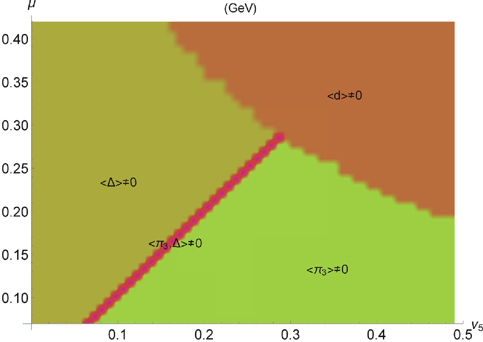Figure1. (color online) Phase diagram of the two-color QCD with two fundamental quarks in the $\mu-\nu_{5}$ plane at zero temperature.

The VEVs of the three condensates are shown as a function of the axial isospin chemical potential and/or temperature in Figs. 2, 3 and 4. These plots demonstrate that the gap of the spin one color superconductor is smaller than the chiral condensate, as revealed in the early studies of the $ N_{c} = 3 $ color superconductivity [1, 72]. We observe that as the temperature increases, all VEVs of the fields decrease, as shown in Fig. 2. The system undergoes a phase transition to a quark-gluon plasma at high temperatures. The order parameters as function of $ \nu_{5} $ for different values of chemical potential and temperature are also shown. The pion superfluid vanishes at high temperature ($ T = 150\; {{\rm{MeV}}} $) and the chiral symmetry is only broken by the scalar diquark condensate, as presented in Fig. 3 for chemical potential $ \mu = 250\; {{\rm{MeV}}} $. The scalar diquark condensate vanishes at high axial isospin density. Simultaneously, the condensation of the axial vector diquark begins. At low temperature $ T = 40\; {{\rm{MeV}}} $, and if the chemical potential is lower than $ 150\; {{\rm{MeV}}} $ or higher than $ 300\; {{\rm{MeV}}} $, the value of the chiral condensate, i.e. the sum of $ \pi_{3} $ and $ \Delta $, is continuous and disappears for dense $ \nu_{5} $. In turn, the system is characterized by the axial vector diquark condensation of d, as is shown in Fig. 4.
Figure2. (color online) Scalar diquark condensate $\Delta $ and axial vector diquark d as a function of T for a given $\mu$ and $\nu_{5}$. The units of $\mu$ and $\nu_{5}$ are ${\rm{GeV}} $.

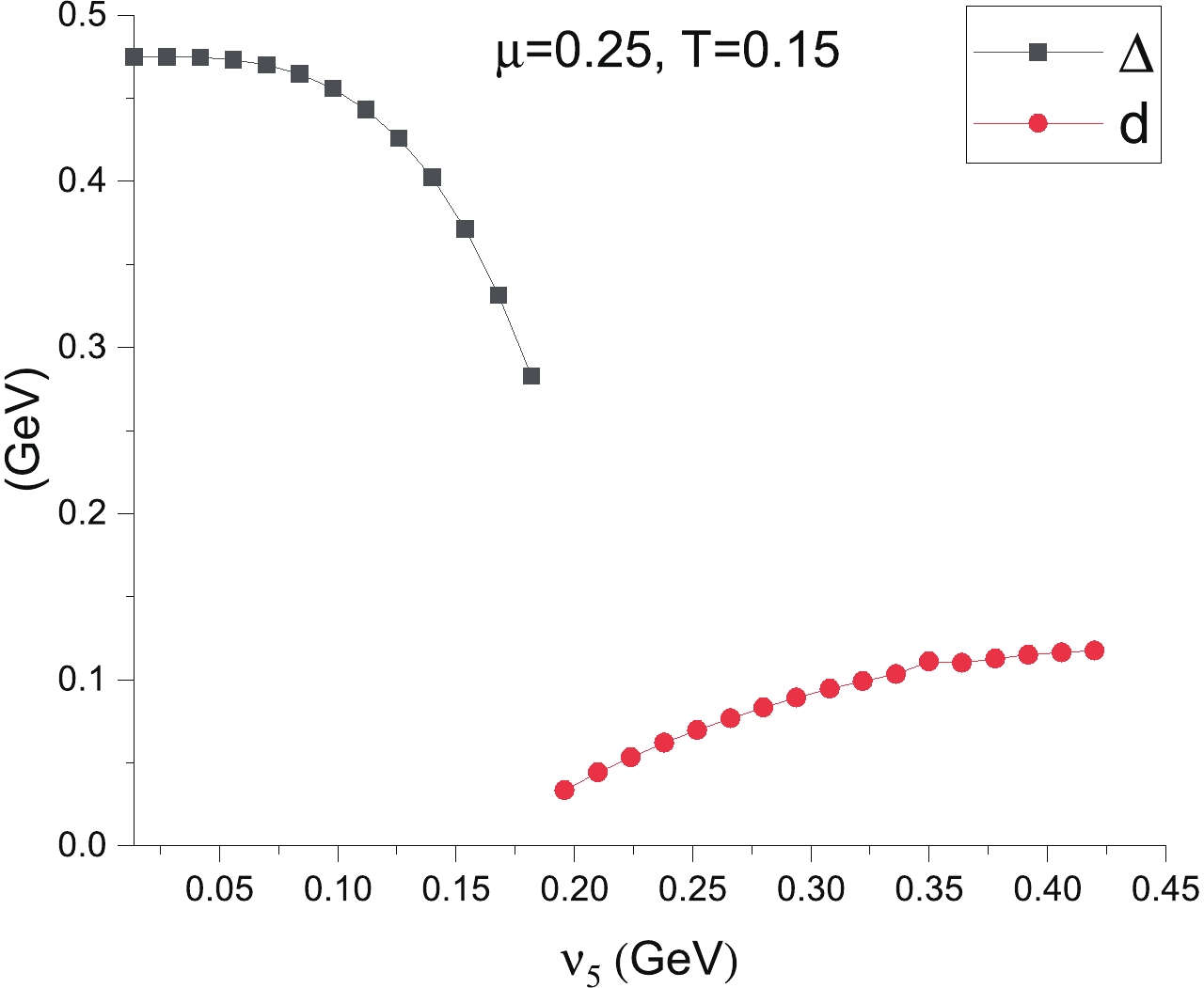Figure3. (color online) Scalar diquark condensate $\Delta $ and axial vector diquark d as a function of $\nu_{5}$ for a given $\mu$ and T. The units of $\mu$ and T are ${\rm{GeV}} $.

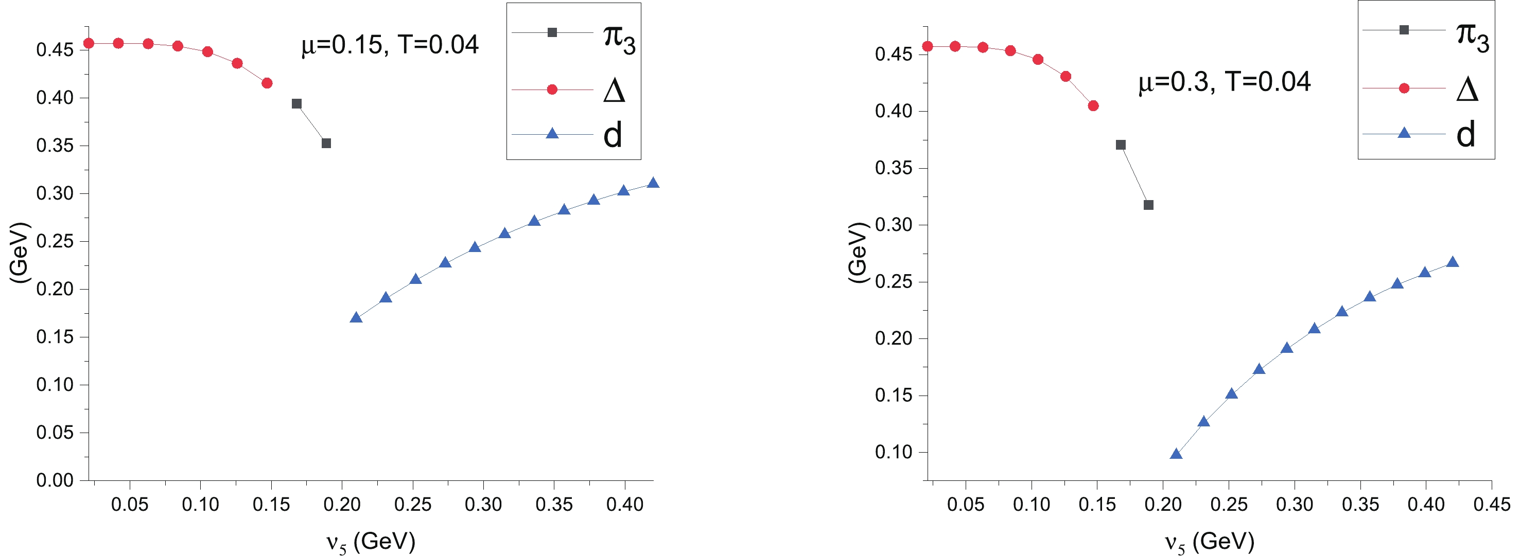Figure4. (color online) Neutral pion condensate $\pi_{3}$, scalar diquark condensate $\Delta $ and axial vector diquark d as a function of $\nu_{5}$ for a given $\mu$ and T. The units of $\mu$ and T are ${\rm{GeV}} $.

In this paper, we proposed that an axial isospin density term $ \nu_{5}\bar{\psi} \gamma_{0} \gamma_{5}\tau_{3}\psi $ is included in the Lagrangian [62-64] to mimic the parallel or anti-parallel EM fields in quark matter. The underlying mechanism is the following: because of their asymmetric electric charges, the $ u, d $ quarks induce an intense electromagnetic triangle anomaly if the EM field strength is at the hadron scale. As we are interested in the pattern of quark-quark paring, we considered in this work a system at finite baryon chemical potential $ \mu $, starting from $ 70\; {{\rm{MeV}}} $. In order to ease the comparison with lattice calculations, we have adopted a two-color QCD toy model to guarantee the positivity of the Euclidean path integral with pseudo-real fermions [4, 7, 8]. In this QCD-like theory, the NJL-type interactions are embedded in the extended global $ {SU}(4) $ symmetry.
Following previous works on anisotopic dense quark matter [4, 7, 8], the chiral rotation in $ {SU}(4) $ space is studied using the low energy effective theory $ \chi {\rm PT} $ at leading order. Using the covariance of the gauge symmetry, we obtained the possible QCD vacuum orientations in several environments. It was shown that there is a qualitative difference between dense baryon systems at finite isospin and axial isospin densities, which originates in the distinct nature of quasi-particles, mesons and baryons (diquarks). We analytically computed the alignment of the ground state to the scalar diquarks, $ \Delta\,( \Delta^{*}) $, axial-vector diquarks, $ d\,(d^{*}) $, and neutral pion meson directions from the usual scalar meson $ \sigma $ condensate in the $ \mu-\nu_{5} $ plane. The possible states of the pion superfluid agree with the results obtained in [56], where the chiral rotation to $ \pi_{3} $ is driven by the electromagnetic anomaly. We emphasize that the neutral $ \pi_{3} $ and charged $ \pi_{\pm} $ lose their degeneracy in the EM fields. It was suggested that the system favors the charged pion instead of neutral pion condensation if more EM anomaly processes are included, such as the box anomaly or the five-point contribution $ \gamma \gamma\to\pi_{3}\pi_{+}\pi_{-} $ [79, 80]. Therefore, it is reasonable that there is a discrepancy between Eq. (23) and the results of charged pion condensation obtained in [75]. In our case, the charged pion condensate is absent for nonzero $ \nu_{5} $ since the axial isospin current is generated by a single triangle anomaly.
Assuming that the condensates involve only real $ \Delta $, d and $ \pi_{3} $, and applying the mean-field approximation, we studied the phase structure of the two-color NJL model. It was shown that the model calculations are consistent with the expectations from $ \chi {\rm PT} $. We remark that a novel result was revealed in the QCD phase diagram, where a co-existent phase appears. It mixes the neutral pion and scalar diquark condensates in a shallow window where $ \mu $ is proportional to $ \nu_{5} $. The relevant thermodynamic quantities at finite temperatures were obtained as well. Using either the $ \chi {\rm PT} $ or NJL models, the two-color calculations can be applied easily to the three-color QCD.
In our simplified model, the back reactions on the electric blind fields have not been taken into account. The coupling of the quark sector to the Polyakov loop is not included and therefore there is no (de)confinement effect [81-83]. Furthermore, a first principles calculation could be pursued by the Dyson-Schwinger equations and/or functional renormalization group approach. As this study was devoted to the properties of the axial isotopically asymmetric dense QCD matter, it could be verified by lattice simulations of the two-color QCD applying similar strategies for finite baryon and isospin chemical potentials.
An application of our analysis to heavy-ion collisions, where strong anti-parallel electric and magnetic fields are produced above and below the reaction plane, is suggested. In addition, we observed that the axial vector diquark condensate develops as a physical ground state in the phase diagram. Its equation-of-state, thermodynamic behavior and transport coefficients, especially its emissivity, could be studied in low-temperature/high-density heavy-ion collision experiments at several worldwide facilities. It also gives reason for further investigations in the case of compact stars.
To summarize, this work explores the phenomenology of the QCD-like matter in different extreme conditions. The study of the two-color QCD serves as a first step towards realistic QCD matter. The subject of a future investigation will be to extend this work to the $ N_{c} = 3 $ QCD matter. We believe that our effort contributes to the general understanding of cold dense strongly interacting matter.
I thank M. Huang, K. Xu and M. Ruggieri for discussions and the comments from T. Schaefer.