Li Cheng ^1,,
, Otto Eberhardt ^2,,
, Christopher W. Murphy ^3,,
,

Corresponding author: Li Cheng, clmamuphy@sina.cn

Corresponding author: Otto Eberhardt, otto.eberhardt@ific.uv.es

Corresponding author: Christopher W. Murphy, cmurphy@bnl.gov

1.Institute of Applied Physics and Computational Mathematics, Beijing 100094, China
2.Instituto de Física Corpuscular, Universitat de València – CSIC, Apt. Correus 22085, E-46071 València, Spain
3.Department of Physics, Brookhaven National Laboratory, Upton, New York, 11973, USA
Received Date:2019-04-16
Available Online:2019-09-01
Abstract:We study the theoretical constraints on a model whose scalar sector contains one color octet and one or two color singlet SU(2)_L doublets. To ensure unitarity of the theory, we constrain the parameters of the scalar potential for the first time at the next-to-leading order in perturbation theory. Moreover, we derive new conditions guaranteeing the stability of the potential. We employ the HEPfit package to extract viable parameter regions at the electroweak scale and test the stability of the renormalization group evolution up to the multi-TeV region. Furthermore, we set upper limits on the scalar mass splittings. All results are given for both cases with and without a second scalar color singlet.

HTML

--> --> -->

The discovery of the 125-GeV Higgs boson at the LHC [1, 2] exemplifies the success of the standard model (SM). Considering experimental precision, the possibility of physics beyond the SM (BSM) is not excluded yet, however, given the null results of the direct search, any BSM physics that is discovered is likely to be more exotic in nature. It is therefore important to determine to what extent different BSM scenarios are viable. Inspired by supersymmetric models, the Two-Higgs-Doublet Model (2HDM) that adds another Higgs doublet is one of the simplest and most commonly studied extensions of the SM. Manohar and Wise (MW), starting from the principle of minimal flavor violation (MFV), proposed an alternative model [3]. It follows from MFV that the scalar sector can only have two representations, the color-singlet and color-octet. Therefore, the authors constructed an extension of the SM by adding a color-octet electroweak doublet scalar. The phenomenology of the model has been studied in detail [4–17], including aspects such as production of scalars, the lower limit of the scalar masses, and possible constraints on the parameter space.
Combining the above motivations, Refs. [18, 19] recently proposed a new model containing aspects of both the MW model and 2HDM. In particular, the scalar sector of the model in consideration consists of two color-singlet electroweak doublets, $ \Phi_{1, 2} $, and one color-octet electroweak doublet, S. The MW model is the limiting case with $ \Phi_2 \to 0 $, whereas the 2HDM is recovered in the limit $ S \to 0 $. Because of the existence of these two limiting cases, we will refer to this model as the 2HDMW. The inclusive character of the 2HDMW model is capable of explaining new physics and is compatible with the established experimental observations. For example, this represents a viable model for LHC physics in terms of h-signal strengths, since they are not necessarily affected at the tree-level. It is also suggested that the 2HDMW can emerge naturally from GUT theories [20–22]. Therefore, the 2HDMW depicts one of the possible physics at the low scale upon breaking down of the more general symmetry. In the meantime, CP violating phases are introduced to the scalar sector in its most general formulation.
Ref. [18] investigated tree-level constraints on the 2HDMW arising from symmetries and perturbative unitarity. A study of LHC phenomenology was also performed, which found that the color-octet scalar added to the 2HDM could produce large corrections to the one-loop couplings of the Higgs boson to two gluons or photons. The study presented in Ref. [19] derived the one-loop beta functions for the scalar couplings in the 2HDMW, and the evolution of the renormalization group equations (RGEs) was then used to place upper limits on the parameters of the model. Similar practices were applied in studies of the the SM [23, 24], MW model [14], and the 2HDM [25–27]. The parameter space was further constrained in Ref. [19] by requiring no Landau poles (LPs) below a certain high-energy scale Λ, the scalar potential being stable and the perturbative unitarity being satisfied at all scales below Λ. The perturbative unitarity constraints imposed on the model in Refs. [18, 19] are of the leading order (LO), and a considerable region in the parameter space survives.
Although instructive, the preceding studies on constraints imposed on the 2HDMW are not yet comprehensive. It is a reasonable expectation that supplementing corrections at higher orders can result in noticeable modifications to the surviving parameter space. However, the behavior of higher order corrections is usually complicated. There is no simple answer to whether their impact is to tighten or relax the viable ranges of couplings. In this study, we utilize the generic tool provided by Refs. [28–30] to explore these perturbative unitarity bounds at next-to-leading order (NLO) and first impose them on color-octet scalar. However, the positivity conditions are only known for 2HDM. Taking an additional color-octet into account, one should reconsider the scalar potential as a whole and secure the existence of the global minimum. Completely solving this problem is extremely challenging. This study is also the first work to expand the set of positivity conditions to both MW and 2HDMW models.
Generally, this work focuses on theoretical constraints of the 2HDMW. An investigation of experimental bounds of the model will be performed in a future study. The rest of the paper is organized as follows: the 2HDMW model is defined in Sec. 2. The theoretical constraints are explained in Sec. 3. Followingly, our results for the surviving parameter space are presented in Sec. 4. Concluding remarks are provided in Sec. 5.

As stated above, the scalar sector of the model consists of two color-singlet electroweak doublets $ \Phi_{1, 2} $, and one color-octet electroweak doublet S. The most general renormalizable potential of the scalar sector is [18, 31]:

$ \begin{split}V_{\rm{gen}}\! =& m_{11}^2\Phi_1^\dagger\Phi_1^{\phantom{\dagger}} \! +\! m_{22}^2\Phi_2^\dagger\Phi_2^{\phantom{\dagger}} \! -\! m_{12}^2 \left( \Phi_1^\dagger\Phi_2^{\phantom{\dagger}} \!+\!\Phi_2^\dagger\Phi_1^{\phantom{\dagger}}\right) \! +\! \displaystyle\frac{1}{2} \lambda_1\left(\Phi_1^\dagger\Phi_1^{\phantom{\dagger}}\right)^2 \\& + \displaystyle\frac{1}{2} \lambda_2\left(\Phi_2^\dagger\Phi_2^{\phantom{\dagger}}\right)^2 \! +\! \lambda_3 \left(\Phi_1^\dagger\Phi_1^{\phantom{\dagger}}\right) \left(\Phi_2^\dagger\Phi_2^{\phantom{\dagger}}\right) \! +\! \lambda_4 \left(\Phi_1^\dagger\Phi_2^{\phantom{\dagger}}\right) \left(\Phi_2^\dagger\Phi_1^{\phantom{\dagger}}\right) \\&+ \displaystyle\frac{1}{2} \left[ \lambda_5 \left(\Phi_1^\dagger\Phi_2^{\phantom{\dagger}}\right)^2 + {\rm h.c.} \right] + \left[ \lambda_6 \left( \Phi_1^\dagger\Phi_1^{\phantom{\dagger}} \right) \left( \Phi_1^\dagger\Phi_2^{\phantom{\dagger}} \right) \right. \\& \left. +\lambda_7 \left( \Phi_2^\dagger\Phi_2^{\phantom{\dagger}} \right) \left( \Phi_1^\dagger\Phi_2^{\phantom{\dagger}} \right) + {\rm h.c.} \right] + 2 m_S^2 {\rm Tr}\left(S^{\dagger i} S^{\phantom{\dagger}}_i\right) \\ & + \mu_1 {\rm Tr}\left(S^{\dagger i} S^{\phantom{\dagger}}_i S^{\dagger j} S^{\phantom{\dagger}}_j\right) + \mu_2 {\rm Tr}\left(S^{\dagger i} S^{\phantom{\dagger}}_j S^{\dagger j} S^{\phantom{\dagger}}_i\right) \\ & + \mu_3 {\rm Tr}\left(S^{\dagger i} S^{\phantom{\dagger}}_i\right) \left(S^{\dagger j} S^{\phantom{\dagger}}_j\right) + \mu_4 {\rm Tr}\left(S^{\dagger i} S^{\phantom{\dagger}}_j\right) \left(S^{\dagger j} S^{\phantom{\dagger}}_i\right) \\ & + \mu_5 {\rm Tr}\left(S^{\phantom{\dagger}}_i S^{\phantom{\dagger}}_j\right) \left(S^{\dagger i} S^{\dagger j}\right) + \mu_6 {\rm Tr}\left(S^{\phantom{\dagger}}_i S^{\phantom{\dagger}}_j S^{\dagger j} S^{\dagger i}\right) \\ & + \nu_1 \Phi_1^{\dagger i}\Phi_{1i}^{\phantom{\dagger}} {\rm Tr}\left(S^{\dagger j} S^{\phantom{\dagger}}_j\right) + \nu_2 \Phi_1^{\dagger i}\Phi_{1j}^{\phantom{\dagger}} {\rm Tr}\left(S^{\dagger j} S^{\phantom{\dagger}}_i\right) \\ & +\left[ \nu_3 \Phi_1^{\dagger i}\Phi_1^{\dagger j} {\rm Tr}\left(S^{\phantom{\dagger}}_i S^{\phantom{\dagger}}_j\right) +\nu_4 \Phi_1^{\dagger i} {\rm Tr}\left(S^{\dagger j} S^{\phantom{\dagger}}_j S^{\phantom{\dagger}}_i\right) \right. \\ &\left.+\nu_5 \Phi_1^{\dagger i} {\rm Tr}\left(S^{\dagger j} S^{\phantom{\dagger}}_i S^{\phantom{\dagger}}_j\right) + {\rm h.c.}\right] + \omega_1 \Phi_2^{\dagger i}\Phi_{2i}^{\phantom{\dagger}} {\rm Tr}\left(S^{\dagger j} S^{\phantom{\dagger}}_j\right) \\ & + \omega_2 \Phi_2^{\dagger i}\Phi_{2j}^{\phantom{\dagger}} {\rm Tr}\left(S^{\dagger j} S^{\phantom{\dagger}}_i\right) +\left[ \omega_3 \Phi_2^{\dagger i}\Phi_2^{\dagger j} {\rm Tr}\left(S^{\phantom{\dagger}}_i S^{\phantom{\dagger}}_j\right)\right. \\ &\left.+\omega_4 \Phi_2^{\dagger i} {\rm Tr}\left(S^{\dagger j} S^{\phantom{\dagger}}_j S^{\phantom{\dagger}}_i\right) +\omega_5 \Phi_2^{\dagger i} {\rm Tr}\left(S^{\dagger j} S^{\phantom{\dagger}}_i S^{\phantom{\dagger}}_j\right) +{\rm h.c.}\right] \\ &+\left[ \kappa_1 \Phi_1^{\dagger i} \Phi_{2i}^{\phantom{\dagger}} {\rm Tr}\left(S^{\dagger j} S^{\phantom{\dagger}}_j\right) +\kappa_2 \Phi_1^{\dagger i} \Phi_{2j}^{\phantom{\dagger}} {\rm Tr}\left(S^{\dagger j} S^{\phantom{\dagger}}_i\right) \right. \\ &\left.+\kappa_3 \Phi_1^{\dagger i} \Phi_2^{\dagger j} {\rm Tr}\left(S^{\phantom{\dagger}}_j S^{\phantom{\dagger}}_i\right) +{\rm h.c.}\right] . \end{split} $

(1)

All interactions between S, $ \Phi_1 $, and $ \Phi_2 $ and the self-interactions are included. In Eq. (1), we use i, j as $ SU(2) $ indices, and the notation $ S_i = S_i^A T^A $, where A is color index. The trace is taken over the color indices.
The physical parameters of this model are the masses of the $ \Phi_1 $ and $ \Phi_2 $ fields, which we denote in the 2HDM as $ m_h $, $ m_H $, and $ m_A $ for the neutral bosons and as $ m_{H^\pm} $ for the charged Higgs particles, as well as the octet masses $ m_R $, $ m_I $ and $ m_{S^\pm} $ for the neutral scalar, neutral pseudoscalar, and the charged octet scalar of the MW model. Moreover, we refer to the two angles of the diagonalization of the mass matrix in the 2HDM sector as α and β, according to the conventions in the literature.
We apply the following conditions to reduce the number of parameters in the scalar potential and the Yukawa potential, defined below in Eq. (2) and Eq. (3), respectively.
● We restrict the 2HDM sector to be CP-conserving.
● Custodial symmetry [32–34]: We adopt the less restrictive method discussed in [18]. The mass degeneracies $ m_{H^\pm} = m_A $ and $ m_{S^\pm} = m_I $ result from custodial symmetry.
● We impose a $ \mathbb{Z}_2 $ symmetry, which is only softly broken by quadratic terms. This prevents tree level flavor changing neutral currents (FCNCs), and further reduces the number of free parameters. The charge assignments we consider are given in Table 1. The original MW study was motivated by the principle of minimal flavor violation [35, 36]. This is in contrast with our approach of imposing $ \mathbb{Z}_2 $ symmetry, which is motivated by the practicality of reducing the number of parameters in the scalar potential while still maintaining some ability to generate flavor effects.

	Φ1	Φ2	S	UR	DR	QL
Type I	?	+	?	?	?	+
Type IIu	?	+	?	?	+	+
Type IId	?	+	+	?	+	+

Table1.$\mathbb{Z}_2$ charge assignments in the 2HDMW that forbid tree level FCNCs. In type IIu (IId), the color-octet scalar S only interacts with up-type (down-type) quarks.

The scalar potential of the model with the aforementioned imposed constraints reads:

$ \begin{split}V_{{\rm {fit}}} =& m_{11}^2\Phi_1^\dagger\Phi_1^{\phantom{\dagger}} \!+\! m_{22}^2\Phi_2^\dagger\Phi_2^{\phantom{\dagger}} \!-\! m_{12}^2 \left( \Phi_1^\dagger\Phi_2^{\phantom{\dagger}} \!+\!\Phi_2^\dagger\Phi_1^{\phantom{\dagger}}\right) \! +\! \displaystyle\frac{1}{2} \lambda_1\left(\Phi_1^\dagger\Phi_1^{\phantom{\dagger}}\right)^2 \\& + \displaystyle\frac{1}{2} \lambda_2\left(\Phi_2^\dagger\Phi_2^{\phantom{\dagger}}\right)^2 + \lambda_3 \left(\Phi_1^\dagger\Phi_1^{\phantom{\dagger}}\right) \left(\Phi_2^\dagger\Phi_2^{\phantom{\dagger}}\right) + \displaystyle\frac{1}{2} \lambda_4 \left[ \left(\Phi_1^\dagger\Phi_2^{\phantom{\dagger}}\right) \right. \\ & \left. + \left(\Phi_2^\dagger\Phi_1^{\phantom{\dagger}}\right) \right]^2 + 2 m_S^2 {\rm Tr}\left(S^{\dagger i} S^{\phantom{\dagger}}_i\right) + \mu_1 \left[ {\rm Tr}\left(S^{\dagger i} S^{\phantom{\dagger}}_i S^{\dagger j} S^{\phantom{\dagger}}_j\right) \right. \\ & \left.+{\rm Tr}\left(S^{\dagger i} S^{\phantom{\dagger}}_j S^{\dagger j} S^{\phantom{\dagger}}_i\right) +2 {\rm Tr}\left(S^{\phantom{\dagger}}_i S^{\phantom{\dagger}}_j S^{\dagger j} S^{\dagger i}\right) \right] \\ & + \mu_3 {\rm Tr}\left(S^{\dagger i} S^{\phantom{\dagger}}_i\right) \left(S^{\dagger j} S^{\phantom{\dagger}}_j\right) + \mu_4 \left[ {\rm Tr}\left(S^{\dagger i} S^{\phantom{\dagger}}_j\right) \left(S^{\dagger j} S^{\phantom{\dagger}}_i\right) \right. \\ & \left. + {\rm Tr}\left(S^{\phantom{\dagger}}_i S^{\phantom{\dagger}}_j\right) \left(S^{\dagger i} S^{\dagger j}\right) \right] + \nu_1 \Phi_1^{\dagger i}\Phi_{1i}^{\phantom{\dagger}} {\rm Tr}\left(S^{\dagger j} S^{\phantom{\dagger}}_j\right) \\ &+\displaystyle\frac{1}{2} \nu_2 \left[ \Phi_1^{\dagger i}\Phi_{1j}^{\phantom{\dagger}} {\rm Tr}\left(S^{\dagger j} S^{\phantom{\dagger}}_i\right) +\Phi_1^{\dagger i}\Phi_1^{\dagger j} {\rm Tr}\left(S^{\phantom{\dagger}}_i S^{\phantom{\dagger}}_j\right) + {\rm h.c.}\right] \\ & +\nu_4 \left[ \Phi_1^{\dagger i} {\rm Tr}\left(S^{\dagger j} S^{\phantom{\dagger}}_j S^{\phantom{\dagger}}_i\right) +\Phi_1^{\dagger i} {\rm Tr}\left(S^{\dagger j} S^{\phantom{\dagger}}_i S^{\phantom{\dagger}}_j\right) + {\rm h.c.}\right] \\ & + \omega_1 \Phi_2^{\dagger i}\Phi_{2i}^{\phantom{\dagger}} {\rm Tr}\left(S^{\dagger j} S^{\phantom{\dagger}}_j\right) +\displaystyle\frac{1}{2} \omega_2 \left[ \Phi_2^{\dagger i}\Phi_{2j}^{\phantom{\dagger}} {\rm Tr}\left(S^{\dagger j} S^{\phantom{\dagger}}_i\right) \right. \\ &\left. +\Phi_2^{\dagger i}\Phi_2^{\dagger j} {\rm Tr}\left(S^{\phantom{\dagger}}_i S^{\phantom{\dagger}}_j\right) + {\rm h.c.}\right] \\ & +\omega_4 \left[ \Phi_2^{\dagger i} {\rm Tr}\left(S^{\dagger j} S^{\phantom{\dagger}}_j S^{\phantom{\dagger}}_i\right) +\Phi_2^{\dagger i} {\rm Tr}\left(S^{\dagger j} S^{\phantom{\dagger}}_i S^{\phantom{\dagger}}_j\right) + {\rm h.c.}\right] , \end{split}$

(2)

where $ \omega_4 = 0 $ in Type I and Type IIu 2HDMW, and $ \nu_4 = 0 $ in the Type IId 2HDMW, which provides four massive and twelve massless parameters. The masses of scalars and their mixing angles are obtained by diagonalizing the mass matrices of this model. The expressions of those physical parameters were presented in Eqs. (6) and (7) in Ref. [18]. An overview over all assumptions, a comparison with the limiting cases of the 2HDM and the MW model, and an account of the free parameters are provided in Table 2.

	MW	dof.	2HDM	dof.	2HDMW	dof.
General	–	(16)	–	(13)	–	(42)
CP conservation	$ {\rm Im}[\nu_{i+2}]=0 $	(14)	$ {\rm Im}[m_{12}^2]=0,\;{\rm Im}[\lambda_{i+4}]=0 $	(10)	$ {\rm Im}[m_{12}^2]={\rm Im}[\lambda_{i+4}]=0 $, $ {\rm Im}[\nu_{i+2}]={\rm Im}[\omega_{i+2}]={\rm Im}[\kappa_i]=0 $	(30)
Custodial symmetry case 1 of Ref.[18]	$ \mu_1=\mu_2=\frac12 \mu_6 $, $ \mu_4=\mu_5 $, $ \nu_2=2\nu_3 $, $ \nu_4=\nu_5^* $	(9)	$ {\rm Im}[m_{12}^2]=0 $, $ {\rm Im}[\lambda_{i+4}]=0 $, $ \lambda_4=\lambda_5 $	(9)	$ {\rm Im}[m_{12}^2]={\rm Im}[\lambda_{i+4}]=0 $, $ \lambda_4=\lambda_5 $, $ \mu_1=\mu_2=\frac12 \mu_6 $, $ \mu_4=\mu_5 $, $ \nu_2=2\nu_3 $, $ \nu_4=\nu_5^* $, $ \omega_2=2\omega_3 $, $ \omega_4=\omega_5^* $, $ \kappa_2=\kappa_3 $	(24)
$ \mathbb{Z}_2 $ symmetry I/IIu	–	(16)	$ \lambda_6=\lambda_7=0 $	(9)	$ \omega_4=\omega_5=\lambda_6=\lambda_7=0 $, $ \kappa_i=0 $	(28)
$ \mathbb{Z}_2 $ symmetry IId	$ \nu_4=\nu_5=0 $	(12)	$ \lambda_6=\lambda_7=0 $	(9)	$ \nu_4=\nu_5=\lambda_6=\lambda_7=0 $, $ \kappa_i=0 $	(28)
Everything I/IIu		(9)		(7)		(16)
Everything IId		(8)		(7)		(16)

Table2.Overview over different model assumptions and their implementation and the number of free parameters ("dof.") in the corresponding scalar potentials. The index i ranges from 1 to 3. The last two lines are combinations of all assumptions and thus represent the CP-conserving custodial $ \mathbb{Z}_2 $ symmetric models used for our fits.

The general Yukawa potential of the 2HDMW in the flavor eigenstate basis is given by

$\begin{split}L_{Y} =& \left(- \eta_1^D {\left( Y_D \right)^a}_b {\bar D}_{R, a }\Phi_1^\dagger Q_L^b - \eta_2^D {\left( Y_D \right)^a}_b {\bar D}_{R, a } \Phi_2^\dagger Q_L^b\right. \\& - \eta_1^U {\left( Y_U \right)^a}_b {\bar U}_{R, a}{\tilde \Phi}_1^\dagger Q_L^b -\eta_S^D {\left( Y_D \right)^a}_b {\bar D}_{R, a}S^\dagger Q_L^b \\&\left.- \eta_S^U {\left( Y_U \right)^a}_b {\bar U}_{R, a }{\tilde S}^\dagger Q_L^b \right) + {\rm h.c.} , \end{split}$

(3)

where the $ \eta_i $ are complex constants^①. In the Type I 2HDMW, we have $ \eta_2^D \equiv 0 $, whereas for Type IIu (IId), $ \eta_1^D\equiv 0 $ and $ \eta_S^D\equiv 0 $ ($ \eta_S^U\equiv 0 $). We use the convention $ {\tilde H}_i = \varepsilon_{ij} H_j^* $, where $ H = \Phi_{1,2},S $, and a, b are flavor indices.

2

-->

3.1.Priors

For our analysis, we make use of the open source package HEPfit [37], which is linked to the Bayesian Analysis Toolkit [38]. Even if experimental constraints are not applied and thus do not necessarily rely on a fitting tool, we chose this set-up for the following reasons: BAT can also deal with flat likelihood distributions, and HEPfit is optimized for a fast evaluation of the constraints. Sampling covers the entire parameter space, such that we cannot miss relevant regions. This is not guaranteed if we use a random scattering approach. Furthermore, the presented HEPfit implementation of the 2HDMW, as well as the MW and 2HDM limiting cases are available [37] and can be used in future HEPfit studies on these models, including the experimental data. More information on HEPfit is provided in Refs. [29, 39].
In our Bayesian fits, we use flat priors for the 2HDMW parameters with the following ranges:

$\begin{aligned}-50<\lambda_i,\mu_i,\nu_i,\omega_i<50\\ -2<\log_{10}(\tan\beta)<2\\ 0 \;{\rm GeV}^2<m_S^2<(1000 \;{\rm GeV})^2.\end{aligned} $

We fix $ \beta-\alpha $ to $ \pi/2 $ to align the light Higgs h with the SM Higgs and reproduce its signal strength values at tree-level. We set $ m_{12}^2 = 0 $, because its value is not relevant in this scenario. We do not require $ m_h = 125 $ GeV in the 2HDMW. This constraint can always be accomplished by adjusting $ m_{12}^2 $. Only in the MW limiting case with $ \Phi_2 = 0 $, we impose that the SM-like Higgs has a mass of $ 125.18\pm0.16 $ GeV [40, 41], which results in an almost fixed $ \lambda_1 $, like in the SM.
2 -->

3.2.Unitarity

The unitarity of the S-matrix can be used to place constraints on the parameters of a theory [42] (see also [14, 28, 43–47]). If a certain combination of parameters becomes too large, an amplitude will appear to be non-unitary at a given order in perturbation theory. We refer to these constraints as perturbative unitarity bounds, or just unitarity bounds, even though the more accurate statement would be the breakdown of the perturbation theory.
Considering only two-to-two scattering, these constraints take the following forms at various orders in perturbation theory:

$\begin{split}&{\rm LO:} \quad \left(a_j^{(0)}\right)^2 \leqslant \frac{1}{4}, \\ &{\rm NLO:} \quad 0 \leqslant \left(a_j^{(0)}\right)^2 + 2 \left(a_j^{(0)}\right) {\rm Re}\left(a_0^{(1)}\right) \leqslant\frac{1}{4} , \\ &{\rm NLO+:} \quad \left[\left(a_j^{(0)}\right) + {\rm Re}\left(a_j^{(1)}\right)\right]^2 \leqslant \frac{1}{4}, \end{split}$

(4)

where $ a_j^{(\ell)} $ is the contribution at the $\ell $th order in perturbation theory to the jth partial wave amplitude. The NLO+ inequality includes the square of the NLO correction, and thus contains some, but not all of the NNLO contributions to the partial-wave amplitude. When considering the scattering of scalars at high energy, only the $ j = 0 $ partial wave amplitude is important. The matrix of partial wave amplitudes is given by

$ \left({{a}_{\bf{0}}}\right)_{i,f} = \frac{1}{16 \pi s} \int_{-s}^0 {\rm d}t \, {\cal{M}}_{i \to f}(s, t) , $

(5)

and we use $ a_0 $ to indicate the eigenvalues of $ {{a}_{\bf{0}}} $.
The two-to-two scattering matrix at the tree level in the neutral, color singlet channel of the 2HDMW model was recently derived in Refs. [18, 19]. As the scalar potential, Eq. (1) contains only quartic interaction terms, and the NLO unitarity bounds can be computed approximately using the algorithm of Ref. [30]. A virtue of this approach is its simplicity, as it only relies on knowledge of the LO partial wave matrix and the one-loop scalar contributions to the beta functions of the theory. This algorithm is built on previous work in Refs. [28, 29], and results for the special case of the 2HDM can be found in those references. The NLO contribution to the eigenvalue is given by a sum of two terms

$ a_0^{(1)} = a_{0, \sigma}^{(1)} + a_{0,\, \beta}^{(1)} . $

(6)

The first term follows from the unitarity of the theory, and it is proportional to the square of the LO eigenvalue

$ a_0^{(1)} = \left(i - \frac{1}{\pi}\right) \left(a_0^{(0)}\right)^2 . $

(7)

The second term depends on the one-loop beta functions of the theory, and it can be written in terms of the well known formula for the perturbations of the eigenvalues of an eigensystem for the which the exact LO solution is known

$ a_{0,\, \beta}^{(1)} = \vec{x}_{(0)}^{\top} \cdot {{a}}_{0,\, \beta}^{(1)} \cdot \vec{x}_{(0)} , $

(8)

where $ \vec{x}_{(0)} $ are the LO eigenvectors and

$ {{a}}_{0,\, \beta}^{(1)} = - \frac{3}{2} \left.{{a}}_{0}^{(0)}\right|_{\lambda_m \to \beta_{\lambda_m}} , $

(9)

with $ \beta_{\lambda_m} $ as the beta function associated with the coupling $ \lambda_m $. The approximation is computed at a scale where the center-of-mass energy is much greater than the other scales in the problem (recently, finite $ m^2/s $ corrections have been studied for colorless scalar SM extensions [46, 47]). Hence, we only start enforcing the unitarity bounds for RGE scales above $ 750 $ GeV$ \:\approx\!\sqrt{10}\:v $, and do not impose unitarity bounds when running from the EW scale to 750 GeV.
We also enforce the smallness of higher order corrections to the partial wave amplitudes with the following constraint [28, 29, 48, 49]

$ R^{\prime} \equiv \frac{\left|a_0^{(1)}\right|}{\left|a_0^{(0)}\right|} < 1 $

(10)

for each eigenvalue of the partial wave matrix, as long as $ a_0^{(0)}>0.01 $.
2 -->

3.3.Boundedness from below

To achieve a potential that is bounded from below, we extract the positivity conditions from the generic potential (1), assuming only that all couplings are real. Setting all but one or two of the real scalar fields to zero, we require the resulting coefficient matrix to be copositive [50].

$ \mu = \mu_1 + \mu_2 + \mu_6 + 2 (\mu_3 + \mu_4 + \mu_5) > 0, $

(11)

$ \mu_1 + \mu_2 + \mu_3 + \mu_4 > 0, $

(12)

$ 14 (\mu_1 + \mu_2) + 5 \mu_6 + 24 (\mu_3 + \mu_4) - 3 \left| 2 (\mu_1 + \mu_2) - \mu_6 \right| > 0, $

(13)

$ 5 (\mu_1 + \mu_2 + \mu_6) + 6 (2\mu_3 + \mu_4 + \mu_5) - \left| \mu_1 + \mu_2 + \mu_6 \right| > 0, $

(14)

$ \nu_1 + \sqrt{\lambda_1 \mu }> 0, $

(15)

$ \nu_1 + \nu_2 - 2|\nu_3| + \sqrt{\lambda_1 \mu}> 0, $

(16)

$ \lambda_1 + \frac14 \mu + \nu_1 + \nu_2 + 2 \nu_3 - \frac{1}{\sqrt{3}}|\nu_4+\nu_5| >0, $

(17)

$ \lambda_1> 0, $

(18)

$ \lambda_2> 0, $

(19)

$ \lambda_3+\sqrt{\lambda_1 \lambda_2}> 0, $

(20)

$ \lambda_3+\lambda_4-|\lambda_5|+\sqrt{\lambda_1 \lambda_2}> 0, $

(21)

$ \frac12(\lambda_1+\lambda_2)+\lambda_3+\lambda_4+\lambda_5-2|\lambda_6+\lambda_7|> 0, $

(22)

$ \omega_1 + \sqrt{\lambda_2 \mu}> 0, $

(23)

$ \omega_1 + \omega_2 - 2|\omega_3| + \sqrt{\lambda_2 \mu}> 0, $

(24)

$ \lambda_2 + \frac14 \mu + \omega_1 + \omega_2 + 2 \omega_3 - \frac{1}{\sqrt{3}}|\omega_4+\omega_5| >0 . $

(25)

We want to stress that these conditions are necessary but not sufficient, since we did not analyze the cases with three or more non-zero fields, leaving the $ \kappa_i $ unconstrained. While pure 2HDM inequalities (18) to (22) have been known before [31, 51], we are not aware of such conditions in the Manohar-Wise model; that is why we derive (11) to (18) in the most general way. Finally, (23) to (25) only appear in the 2HDMW.
In our simplified potential $ V_{{\rm {fit}}} $, the positivity conditions reduce to

$\begin{split}\;\;&\mu' = 4\mu_1 + 2\mu_3 + 4\mu_4 > 0, \qquad 5 \mu_1 + 3 \mu_3 + 3 \mu_4 - \left| \mu_1 \right| > 0, \\ &\nu_1 + \sqrt{\lambda_1 \mu'}> 0, \qquad \nu_1 + 2\nu_2 + \sqrt{\lambda_1 \mu'} > 0, \\& \lambda_1 + \frac14 \mu' + \nu_1 + 2\nu_2 - \frac{2}{\sqrt{3}}|\nu_4| > 0, \qquad\lambda_1> 0, \qquad \lambda_2> 0, \\& \lambda_3+\sqrt{\lambda_1 \lambda_2} > 0, \qquad \lambda_3+2\lambda_4+\sqrt{\lambda_1 \lambda_2} > 0, \\& \omega_1 + \sqrt{\lambda_2 \mu'}> 0, \qquad \omega_1 + 2\omega_2 + \sqrt{\lambda_2 \mu'}> 0, \\& \lambda_2 + \frac14 \mu' + \omega_1 + 2\omega_2 - \frac{2}{\sqrt{3}}|\omega_4| > 0. \end{split}$

(26)

2 -->

3.4.Positivity of the mass squares

Additional bounds are derived from requiring the masses of the colored scalars to be real:

$ \begin{split}& \nu_1 c_{\beta}^2 + \omega_1 s_{\beta}^2 > - \frac{4 m_S^2}{v^2} , \\& (\nu_1 + 2 \nu_2) c_{\beta}^2 + (\omega_1 + 2 \omega_2) s_{\beta}^2 > - \frac{4 m_S^2}{v^2} . \end{split}$

(27)

with $ v = \sqrt{v_1^2 + v_2^2} \approx 246 $ GeV, and where $ s_{\beta} $ and $ c_{\beta} $ are the sine and cosine of β, respectively, with $ \tan\beta = v_1 / v_2 $. We must have $ m_S^2 > 0 $, such that the vacuum preserves $ SU(3)_C $. The mass splitting between the colored states is

$ \frac{2}{v^2} \left(m_R^2 - m_{S^{\pm}}^2\right) = \nu_2 c_{\beta}^2 + \omega_2 s_{\beta}^2 , $

(28)

and $ m_{S^{\pm}}^2 = m_I^2 $ owing to custodial symmetry.
2 -->

3.5.Renormalization group stability

Thus far, we only discussed theory constraints at the electroweak scale. Assuming the validity of the model up to some higher scale imposes bounds on the parameters: Scenarios that define a viable model at $ m_Z $ could feature one (or more) quartic couplings with unstable behavior under the renormalization group evolution to a higher scale. This could be due to a Landau pole, however also the boundedness-from-below criteria described in Sec. 3.3 should be fulfilled at any scale. Furthermore, the unitarity conditions should be applied at least above some scale, $ \mu_u $, as they are computed in the limit $ \mu_u\gg \sqrt{\lambda_i} v $ with $ \lambda_i $ denoting quartic coupling of the theory. Here, we chose $ \mu_u = 750 $ GeV, as in Ref. [29]. We only take into account the quartic coupling terms from [19] and neglect the contributions of Yukawa and gauge couplings to the RGEs. In Ref. [19], it was shown how the parameter space is constrained in three cases where $ \log_{10}(\Lambda/1\ {\rm GeV}) = $10, 13, 19 if LO unitarity and 2HDM stability are applied.

While the boundedness-from-below constraints are trivial, we discuss the different unitarity constraints in the 2HDMW, before considering higher scales and the effect of the theory constraints on the physical parameters for both the 2HDMW and the MW model. Due to the large number of degrees of freedom, we present the direct comparison of model parameters in most cases. The results are also translated into physical parameters, such as scalar masses.
The contours in figures presented below are the 100% posterior probability regions. If we change the prior distribution of tanβ, for instance, replacing a flat $ \log_{10}(\tan\beta) $ by a flat tanβ prior, this will modify the shape of the posterior distributions (probably only slightly), however it will not modify the 100% limit.
2

-->

4.1.Different unitarity constraints

In Fig. 1, we show the effects of LO, NLO, and NLO+ criteria on the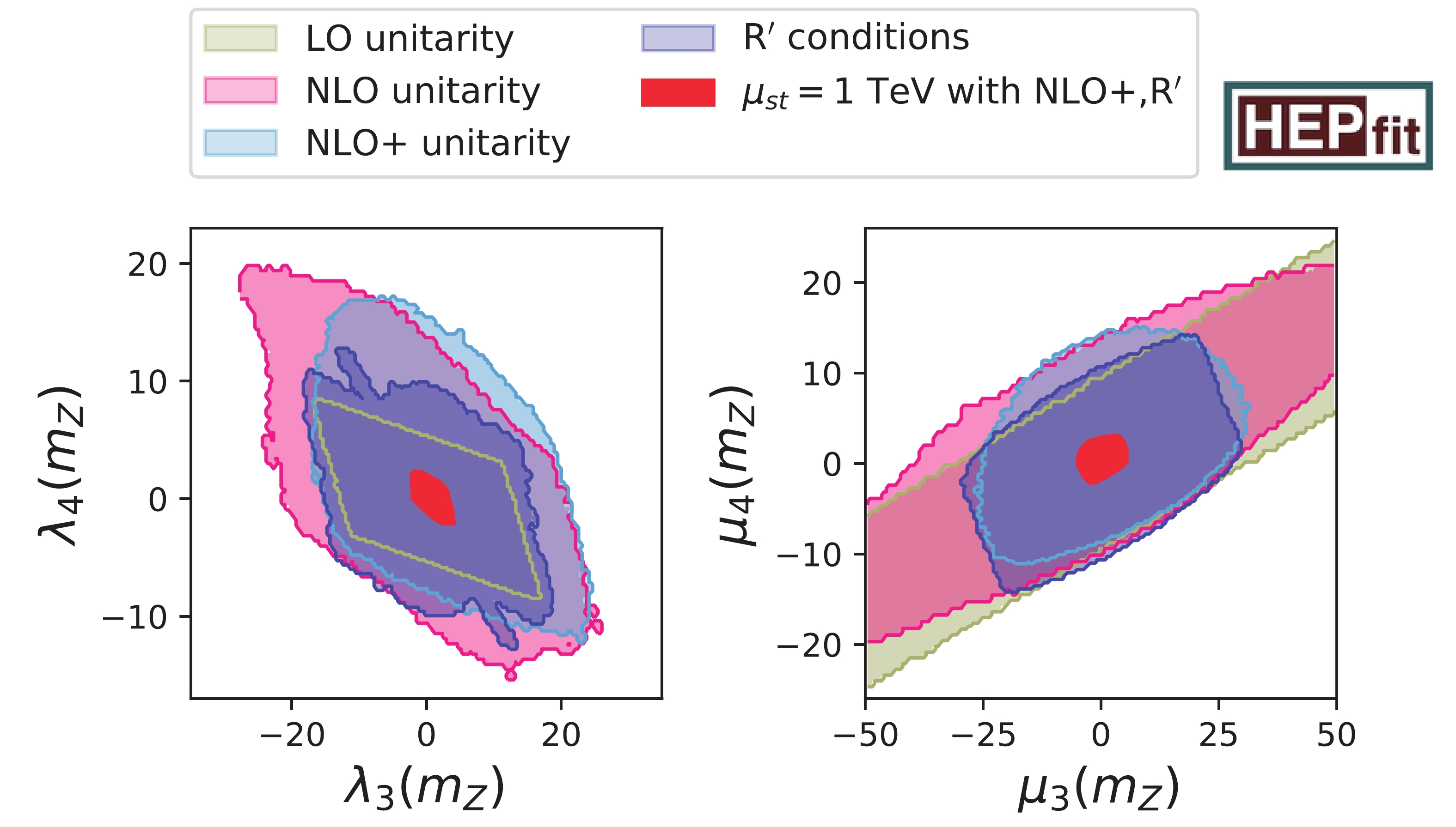 $ \lambda_4 $ vs. $ \lambda_3 $ and $ \mu_4 $ vs. $ \mu_3 $ planes, as well as the impact of the R′ conditions explained in Sec. 3.2 at the electroweak scale. These bounds are calculated without running the renormalization-group equations, except for the red region. We observe that – contrary to the 2HDM case, c.f. Fig. 2 of Ref. [29] – the quartic couplings enjoy more freedom if we apply NLO(+) or the R′ criteria instead of the LO unitarity. The reason for this is that the LO unitarity conditions only depend on a few quartic couplings and disallow extreme values for them, while in the NLO(+) case, large quartic couplings can be compensated by tuning some of the other quartic couplings. Along the diagonal of the left hand panel of Fig. 1, we can observe the consequence of not applying the R′ criteria if the LO unitarity condition is accidentally small: in the small strip with $ |\lambda_4+\lambda_3|\leqslant 0.01 $, the quartic coupling $ \lambda_4 $ can be larger than $ 11 $ in magnitude. If we compare all sets of unitarity constraints with the region that is stable at least up to 1 TeV and compatible with NLO+ unitarity and the R′ conditions, we observe that the latter is a very strong bound. Here, we stress that we recommend to use the NLO(+) unitarity conditions only at scales significantly larger than the electroweak vev, because beyond LO, the quartic couplings are running couplings evaluated at an energy much larger than v.
Figure1. (color online) Comparison of different unitarity bounds in $ \lambda_4 $ vs. $ \lambda_3 $ and $ \mu_4 $ vs. $ \mu_3 $ planes at electroweak scale. Bounds shaded by colors other than red are obtained without running of renormalization-group. Tree-level unitarity constrains the quartic couplings to beige areas; two sets of one-loop conditions NLO and NLO+ force couplings to stay within pink and light blue regions, respectively. The purple contour delimits the area compatible with R′ conditions. Different unitarity bounds at the electroweak scale need to be compared to the regions with stable running, including unitarity up to a scale of 1 TeV (red).

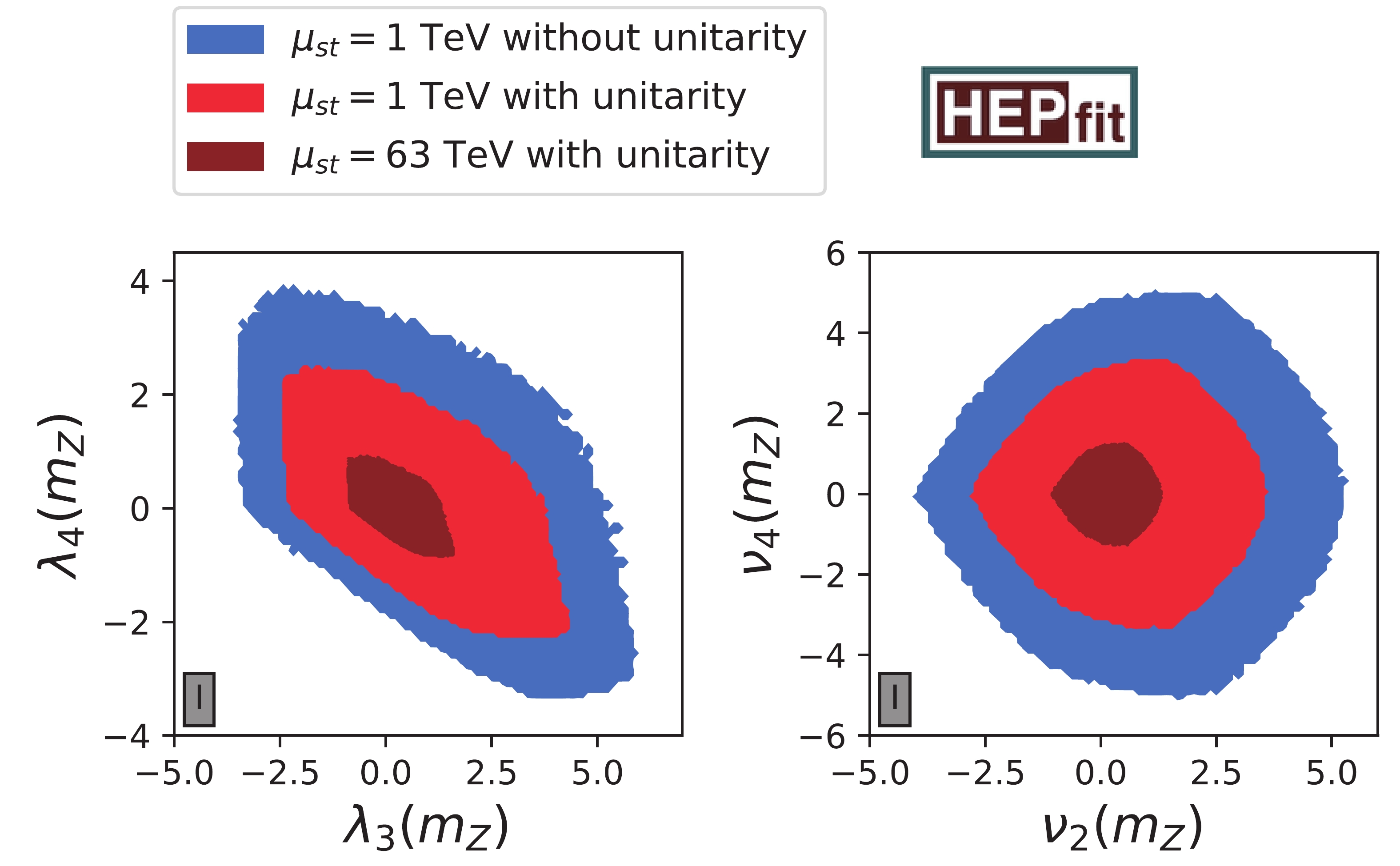Figure2. (color online) RG stability in $ \lambda_4 $ vs. $ \lambda_3 $ and $ \nu_4 $ vs. $ \nu_2 $ planes of 2HDMW of type I at the electroweak scale. Blue contours represent all scenarios that lead to a stable potential up to 1 TeV without imposing any unitarity constraint, whereas NLO+ unitarity and R′ are added to the set of constraints for red regions. The dark red region is compatible with all theory bounds and with a stable potential up to $ 63 $ TeV.

2 -->

4.2.Combination of all theoretical constraints

In Fig. 2, we illustrate the combination of the theory constraints with stability up to a certain scale in the $ \lambda_4 $ vs. $ \lambda_3 $ and $ \nu_4 $ vs. $ \nu_2 $ planes as representative examples of the 2HDMW. The limits obtained from the global fit to all quartic couplings of the 2HDMW and the MW limiting case can be found in Table 3. In this section, we analyze three different scenarios: in the first case, we run all quartic couplings to the stability scale of $ \mu_{st} = 1 $ TeV, whilst at each iteration of the RG evolution controlling whether the potential is bounded from below and whether all quartic couplings are in the perturbative regime, which is smaller than $ 4\pi $ in magnitude. We find that with these constraints, the absolute value of the quartic couplings at the electroweak scale cannot exceed limits between $ 3.3 $ and $ 8.5 $ ($ 1.7 $ and $ 7.5 $) without applying any unitarity bound to the 2HDMW (MW). This has to be confronted with the second scenario, in which we add the NLO+ unitarity constraints as well as the R′ criteria at scales above $ 750 $ GeV to the previous fit. The impact on the parameters is quite sizable: in Fig. 2, we see that the allowed regions shrink by a factor of 1.5 to 2. The maximally allowed values for the quartic couplings range from $ 2.2 $ to $ 5.7 $ in the 2HDMW and from $ 1.3 $ to $ 5.6 $ in the MW, as shown in Table 3. For comparison, the theory-only upper limit on the quartic couplings of the 2HDM is $ 5.75 $ [29]. Finally, we impose that the scalar potential with all discussed theory bounds is stable up to even higher scales $ \Lambda $. Originally, high scales of $ 10^{4.8} $, $ 10^{7.6} $, $ 10^{12} $ and $ 10^{19} $ GeV were to be tested in evenly spaced steps in the logarithm of $ \log_{10} \Lambda $ towards the Planck scale, however our fitting set-up became unstable beyond $ 10^{4.8} $ GeV. If we choose $ 10^{4.8} $ GeV$ \approx 63 $ TeV as our high scale example, all parameters have to be within the range of $ -1.8 $ and $ 2.2 $ in the 2HDMW and between $ -1.6 $ and $ 2.2 $ in the MW. Hence, the limits at $ 63 $ TeV are stronger by a factor of about $ 2/5 $ with respect to the ones obtained with stability at 1 TeV. As a complete illustration, we arrange pairwise correlations of the bounds between all the couplings in Figs. 4 and 5 in the Appendix.

Unitarity $ \mu_{st} $	2HDMW limits					MW limits
	–	LO	NLO+,R'	NLO+,R'		–	LO	NLO+,R'	NLO+,R'
	1 TeV	1 TeV	1 TeV	63 TeV		1 TeV	1 TeV	1 TeV	63 TeV
$ \lambda_1 $	[0, 3.9]	[0, 3.9]	[0, 2.7]	[0, 1.0]		$ 0.2585\pm 0.0007 $
$ \lambda_2 $	[0, 3.9]	[0, 3.9]	[0, 2.7]	[0, 1.0]		–
$ \lambda_3 $	[?3.4, 5.8]	[?3.2, 5.5]	[?2.4, 4.2]	[?0.9, 1.6]		–
$ \lambda_4 $	[?3.3, 3.8]	[?3.2, 3.5]	[?2.2, 2.5]	[?0.9, 0.9]		–
$ \mu_1 $	[?5.5, 6.0]	[?5.3, 5.8]	[?3.8, 4.1]	[?1.5, 1.4]		[?5.3, 5.8]	[?5.3, 2.0]	[?3.6, 4.0]	[?1.4, 1.2]
$ \mu_3 $	[?8.5, 7.8]	[?8.1, 7.7]	[?5.2, 5.7]	[?1.8, 2.2]		[?8.5, 7.5]	[0.0, 4.4]	[?5.1, 5.6]	[?1.6, 2.2]
$ \mu_4 $	[?3.7, 4.9]	[?3.3, 4.8]	[?2.3, 3.2]	[?0.9, 1.2]		[?3.6, 4.8]	[?4.0, 2.3]	[?2.1, 3.1]	[?0.7, 1.2]
$ \nu_1 $	[?4.7, 6.3]	[?4.5, 5.6]	[?3.1, 4.6]	[?1.2, 1.7]		[?1.7, 6.3]	[?1.2, 6.4]	[?1.3, 4.3]	[?0.8, 1.6]
$ \nu_2 $	[?4.0, 5.2]	[?3.6, 5.0]	[?2.7, 3.5]	[?1.1, 1.3]		[?3.3, 5.1]	[?6.2, 6.4]	[?2.3, 3.4]	[?1.0, 1.3]
$ \nu_4 $	[?5.0, 5.0]	[?4.8, 4.7]	[?3.3, 3.3]	[?1.3, 1.3]		[?4.6, 4.5]	[?7.6, 7.7]	[?2.9, 2.9]	[?1.1, 1.1]
$ \omega_1 $	[?4.7, 6.3]	[?4.5, 6.0]	[?3.1, 4.5]	[?1.2, 1.7]		–
$ \omega_2 $	[?4.0, 5.2]	[?3.9, 5.1]	[?2.8, 3.5]	[?1.1, 1.3]		–
$ \omega_4 $	[?4.9, 4.9]	[?4.8, 4.7]	[?3.2, 3.3]	[?1.3, 1.3]		–
$ m_A-m_H $ [GeV]	[?390, 440]	[?340, 400]	[?340, 360]	[?210, 230]		–
$ m_R-m_I $ [GeV]	[?320, 370]	[?280, 330]	[?260, 310]	[?170, 190]		[?250, 300]	[?100, 230]	[?180, 250]	[?150, 180]

Table3.Limits on quartic couplings and two mass differences with different assumptions. Second to fourth columns list 2HDMW results. Note that $ \nu_4 $ ($ \omega_4 $) is only non-zero in the case(s) of the type I, IIu (IId) 2HDMW. Columns five to seven contain the results of the MW limiting case. In this case, $ \lambda_1 = m_h^2/v^2 $.

In the MW limiting case, the role of $ \lambda_1 $ is different, as it is the only parameter that the mass of the SM-like Higgs depends on; it is thus basically fixed by the Higgs mass measurements. Moreover, we do not impose any $ \mathbb{Z}_2 $ symmetry on the MW model, and thus we treat $ \nu_4 $ as a free parameter. The main difference between the limits on quartic couplings in the 2HDMW and MW models is in the extent of negativity of $ \nu_1 $. Since $ \lambda_1 $ is fixed in the MW model, the positivity of the model limits the size of $ \nu_1 $. The Higgs trilinear coupling is sensitive to $ \nu_1 $ at the one-loop level. Thus, larger values of $ \nu_1 $ are advantageous for observation attempts of the double-Higgs boson production at the LHC.
Comparing our results with those of Ref. [19], we find that our permitted ranges for the quartic couplings assuming stability and NLO unitarity up to 63 TeV are more or less of the same size, as previous limits using LO unitarity and no MW positivity up to 2×10⁴ TeV.
The limits on quartic couplings can be translated into bounds on physical model parameters. As in the 2HDM, we observe strong restrictions of the differences between $ m_H^2 $ and $ m_A^2 $ [29, 49], however also $ m_I^2 $ cannot deviate very much from $ m_R^2 $, as shown in Fig. 3. The former mass square difference depends on the values of the $ \lambda_i $, while $ m_R^2-m_I^2 $ is proportional to $ \nu_2 c^2_\beta+\omega_2 s^2_\beta $, see Eq. (28). The linear dependence of the upper limit of the mass splittings for light $ m_H $ and $ m_R $ arises by requiring both masses to be positive. This feature does not appear in the analogous limit in Figure 6 of Ref. [29], because the mass splittings in that figure are plotted against the mass of a third Higgs boson. Fittings to the mass differences $ m_A-m_H $ and $ m_R-m_I $ in the three mentioned scenarios yield upper bounds between $ 440 $ GeV and $ 170 $ GeV in the 2HDMW and between $ 300 $ GeV and $ 150 $ GeV in the MW model, as shown in the last two rows of Table 3. Similarly as in the 2HDMW, the theory-only limit on the mass splitting in the 2HDM is 360 GeV [29]. Even if Figs. 2 and 3 were obtained for the Type I 2HDMW, the 2HDMW limits in Table 3 are valid for all three types, while either $ \nu_4 $ or $ \omega_4 $ have to be set to zero, depending on the type.
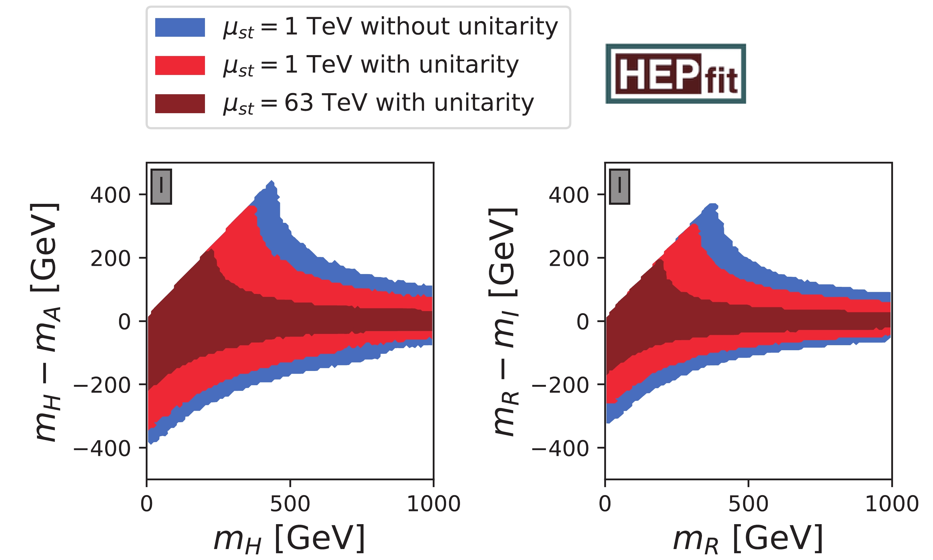Figure3. (color online) Comparison of different stability scales in $ m_H-m_A $ vs. $ m_H $ and $ m_R-m_I $ vs. $ m_R $ planes of Type I 2HDMW. Color coding is described in Fig. 2.

The NLO unitarity bounds were studied on the 2HDMW, which extends the scalar sector of 2HDM with an additional color octet scalar. Although less constraining than the LO unitarity bounds at the electro-weak scale, the NLO unitarity constraints become stronger when approaching higher scales greater than 1 TeV. However, compared with the MW model, which is the limiting case of 2HDMW, common quartic couplings, i.e. μ's and ν's, are allowed for larger ranges under these constraints.
We derived a set of necessary conditions to bound the 2HDMW potential from below for the first time. These conditions constrain most of the quartic couplings with the exception of a few. They are also applicable to the limiting case of the MW model.
Finally, we have combined all theoretical constraints and found limits of the couplings assuming stability at different scales. Requiring a stable potential at a higher scale favors smaller mass differences between pairs of neutral scalars, such as $ m_A-m_H $ and $ m_R-m_I $.
The next step would be a study combining experimental constraints, for which our publicly available HEPfit implementation could be used.
We thank C. Murgui, A. Pich and G. Valencia for fruitful discussions. We thank the INFN Roma Tre Cluster, where most of the fits were performed.

For the sake of completeness, we provide the two-dimensional correlations of the 2HDMW in Fig. 4 and Fig. 5. The former also contains the MW subset, while the latter includes 2HDM correlations.
Figure4. (color online) Pairwise correlations of bounds between all couplings at different scales. The colored scheme of representing different constraints is the same as that of Fig. 2. The cyan dashed box contains MW parameters.

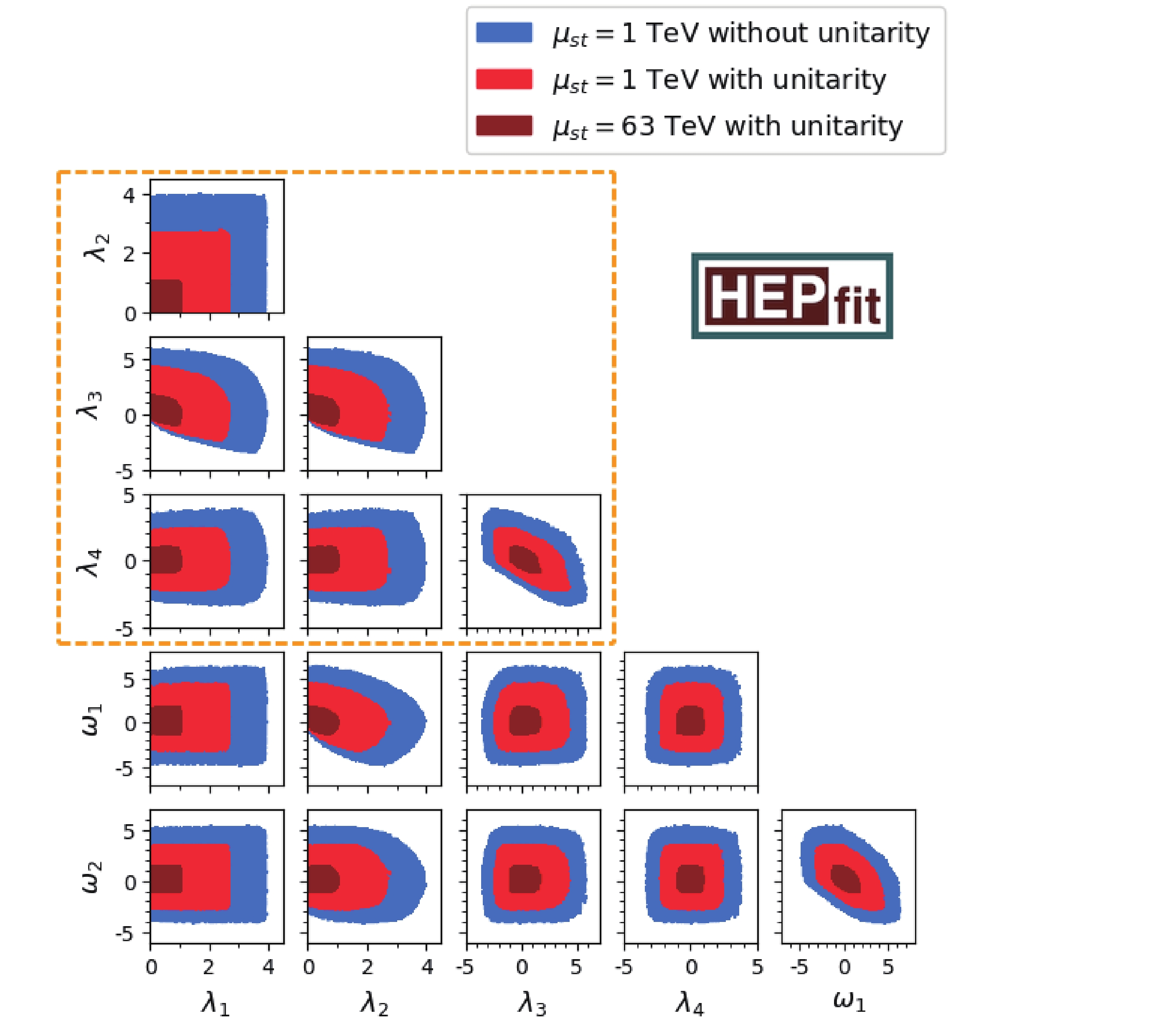Figure5. (color online) Pairwise correlation of bounds between all couplings at different scales. The colored scheme of representing different constraints is the same as that of Fig. 2. The orange dashed box contains 2HDM parameters.