1.School of Physics and Information Engineering, Shanxi Normal University, Linfen 041004 2.DAMTP, Centre for Mathematical Sciences, University of Cambridge, Wilberforce Road, Cambridge CB3 0WA 3.Department of Physics, National Tsing Hua University, Hsinchu 300 4.National Center for Theoretical Sciences, Hsinchu 300 Received Date:2018-10-10 Available Online:2019-02-01 Abstract:We investigate the power spectra of the CMB temperature and matter density in the running vacuum model (RVM) with the time-dependent cosmological constant of $ \Lambda = 3 \nu H^2 + \Lambda_0 $, where $ H $ is the Hubble parameter. In this model, dark energy decreases in time and decays to both matter and radiation. By using the Markov chain Monte Carlo method, we constrain the model parameter $ \nu $ as well as the cosmological observables. Explicitly, we obtain $ \nu \leqslant 1.54 \times 10^{-4} $ (68% confidence level) in the RVM with the best-fit $\chi^2_{\mathrm{RVM}} = 13968.8$, which is slightly smaller than $\chi^2_{\Lambda \mathrm{CDM}} = 13969.8$ in the $\Lambda{\rm{CDM}}$ model of $ \nu=0 $.
HTML
--> --> --> 1.IntroductionOne of the most important recent cosmological observations is that our universe is undergoing a late-time accelerating expansion phase, which is realized by introducing dark energy [1]. Among the many possible dark energy scenarios, the simplest one is the $ \Lambda {\rm{CDM}}$ model, in which a cosmological constant $ \Lambda $ is introduced in the gravitational theory, predicting a constant energy density. Although this model agrees very well with the current cosmological observations, it has several limitations such as “fine-tuning” [2,3] and “coincidence” [4, 5] problems. The running vacuum model (RVM) is one of the popular models used to solve the latter problem [6-17]. In the RVM, instead of a constant, $ \Lambda $ is defined as a function of the Hubble parameter $ H $, and it decays to matter (nonrelativistic fluid) and radiation (relativistic fluid) in the evolution of the universe, leading to the same order of magnitude for the energy densities of dark energy and dark matter [18-33]. Unlike the scalar tensor dark energy theory, such as the simplest realistic scalar field dynamic model [34,35], the RVM has no Lagrangian formula, indicating that this model is an effective theory from some other fundamental gravity theories. One possible origin of the RVM is the quantum effects induced by the cosmological renormalization group, resulting in $ \Lambda = 3\nu H^2 + $$ \Lambda_0 $[36-45] with $ \nu $ and $ \Lambda_0 $ constants. It has been shown in Ref. [46] that the RVM with $ \nu=0 $, i.e., the $ \Lambda {\rm{CDM}}$ limit, is not favored by the observational data, whereas the best-fit for the model occurs at $ \nu=4.8 \times 10^{-3} $, implying that the RVM with $ \nu>0 $ could describe the evolution of our universe well. Results with similar constraints on $ \nu $ have also been given in other types of the RVMs [47-51]. Hence, it is interesting to investigate the matter power spectrum and cosmic microwave background radiation (CMB) temperature fluctuation in this scenario to see if the model is indeed better than the $ \Lambda {\rm{CDM}}$. In this paper, we will derive the growth equations of matter and radiation density fluctuations with the linear perturbation theory and illustrate the matter and CMB temperature power spectra, which can significantly deviate from the $ \Lambda {\rm{CDM}}$ prediction. We will show that the parameter $ \nu $ will be further constrained when the observational data from Planck 2015 is taken into consideration. Furthermore, that the constraint on the RVM obtained in this study is approxiamtely the same order of magnitude as that given in Ref. [52]①), indicating that the CMB photon power spectrum provides a strong constraint on the RVM. In principle, dark energy has to be dynamical, and its density fluctuation should be taken into account when the dark energy decay model is considered. In order to investigate the dynamics of dark energy, the running vacuum energy should be rewritten as a Lorentz scalar at the field equation level. For example, in Refs. [53-56], the cosmological constant is rewritten as $ \Lambda = \Lambda(H) $ with $ H=\nabla_{\mu} U^{\mu}/3 $. In this study, we follow the perturbation method in Refs. [56-59], with which dark energy simultaneously decays to relativistic and nonrelativistic matter and dilutes the density fluctuation. We will also use the Markov chain Monte Carlo (MCMC) method to perform the global fit with the current observational data to further constrain the model. The remainder of this paper is organized as follows. In Section 2, we introduce the RVM and review the background evolutions of matter, radiation, and dark energy. In Section 3, we calculate the linear perturbation theory and present the power spectra of the matter density distribution and CMB temperature by the CAMB program [60]. In Section 4, we use the CosmoMC package [61] to fit the model from the observational data. The conclusions are presented in Section 5.
2.Running vacuum modelThe Einstein equation of the RVM is given by
where $ \kappa^2 = 8 \pi G $, $ R=g^{\mu \nu} R_{\mu \nu} $ is the Ricci scalar, $ \Lambda=\Lambda(H) $ is the time-dependent cosmological constant, and $ T_{\mu \nu}^M $ is the energy-momentum tensor of matter and radiation. In the Friedmann-Lema?tre-Robertson-Walker (FLRW) metric of $ {\rm d}s^2 = a^2(\tau) [ -{\rm d}\tau^2 + \delta_{ij} {\rm d}x^i {\rm d}x^j ] $, the Friedmann equations are derived as
where $ \tau $ is the conformal time, $ H={\rm d}a/(a {\rm d} \tau) $ represents the Hubble parameter, $ \rho_M=\rho_m+\rho_r $ ($ P_{M}=P_m+P_r=P_r $) corresponds to the energy density (pressure) of matter and radiation, and $ \rho_{\Lambda} $ ($ P_{\Lambda} $) is the energy density (pressure) of the cosmological constant. From Eq. (1), we have
In Eq. (1), we consider $ \Lambda $ to be a function of the Hubble parameter, given by [36-45]
$\Lambda = 3\nu {H^2} + {\Lambda _0},$
(6)
where $ \nu $ and $ \Lambda_0 $ are two free parameters. To avoid the negative dark energy density in the early universe, we focus on the RVM with $ \nu \geqslant 0 $ in our investigation. Substituting Eq. (6) into the conservation equation, $ \nabla^{\mu} (T^M_{\mu \nu}+T^\Lambda_{\mu \nu}) = 0 $, we have
where $ \xi=1-\nu $ and $ \rho_{a}^{(0)} $ is the energy density of $ a $ (matter or radiation) at $ z=0 $.
3.Linear perturbation theoryBecause the RVM with the strong coupling $ Q_l $, corresponding to $ \nu \sim \mathcal{O}(1) $, cannot describe the evolution of the universe [47, 49], we only focus on the case of $ \nu \ll 1 $. Note that $ \nu $ is taken to be non-negative, i.e., $ \nu \geqslant 0 $, to avoid $ \rho_{\Lambda}<0 $ in the early universe. The calculation follows the standard linear perturbation theory with the synchronous gauge [62]. The metric is given by
$ i,j=1,2,3 $, $ h $ and $ \eta $ are two scalar perturbations in the synchronous gauge, and $ \hat{k} = \vec{k}/ k $ is the k-space unit vector. From $ \nabla^{\mu} (T^M_{\mu \nu}+T^\Lambda_{\mu \nu}) = 0 $, with $ \delta T^0_0 = \delta \rho_M $, $ \delta T^0_i = -T^i_0 =$$ (\rho_M+P_M) v^i_M $, and $ \delta T^i_j = \delta P_M \delta^i_j $, we can obtain the matter and radiation density perturbations, given by [56-59],
where $ \delta_l \equiv \delta \rho_l / \rho_l $ and $ \theta_l = ik_i v^i_l $ are the density fluctuation and the divergence of the fluid velocity, respectively. Note that Eqs. (13) and (14) describe the evolutions of the density fluctuations of the perfect fluids without the interactions between them. To consider the interactions between any two fluids, these equations should be further modified. Taking the photon-proton interaction as an example, the additional term, $ a n_e \sigma_T (\theta_b - \theta_{\gamma}) $, must be added at the right-hand side of Eq. (14) when $ l=\gamma $; further details of the equations can be found in Ref. [62]. In Eqs. (13) and (14), it can be observed that the last terms in the two equations slow down the increase of $ \delta_l $ and $ \theta_l $ if $ \nu $ in Eq. (9) is positive. To demonstrate how the running vacuum scenario in Eq. (6) influences the physical observables, we used the open-source program CAMB [60], in which we modified the background density evolutions and the evolution equations of $ \delta $ and $ \theta $ in terms of Eqs. (10), (13), and (14). By taking $ 1 \gg \nu \geqslant 0 $, most of the particles are created at the end of inflation, whereas the energy density from the dark energy decay is tiny, implying that the RVM has the same initial conditions as that of the $ \Lambda $ CDM model. In addition, the matter-radiation equality $ z_{eq} $ slightly changes, as shown by
In Fig. 1, we present the matter power spectrum $ P(k) \sim \langle \delta_m^2(k) \rangle $ as a function of the wave number $ k $ with $ \nu=0 $ (solid line), $ 10^{-3} $ (dashed line), $ 5 \times 10^{-3} $ (dotted line), and $ 10^{-2} $(dash-dotted line). As discussed earlier in this section, the matter density fluctuation is diluted by the creation of particles so that the results of $ P(k) $ for a large $ k $ and $ \nu $ in the RVM significantly deviate from that of the $ \Lambda $ CDM model (solid line). Figure1. (color online) The matter power spectrum ${P(k)}$ as a function of the wavelength k with ${\nu=0}$ (solid line), ${10^{-3}}$ (dashed line), ${5 \times 10^{-3}}$ (dotted line), and ${10^{-2}}$ (dash-dotted line), where the boundary conditions are taken to be ${\Omega_b h^2=2.23\times 10^{-2}}$, ${\Omega_c h^2=0.118}$, ${h=0.68}$, ${A_s=2.15 \times 10^{-9}}$, ${n_s=0.97}$, ${\tau=0.07}$, and ${ \Sigma m_{\nu}=0.06}$ eV, respectively.
Figure 2 shows the CMB temperature spectra of (a) $ l(l+1)C_l/2\pi $ and (b) $ \Delta C_l/C_l=(C_l^{\rm RVM}-C_l^{\rm \Lambda CDM})/C_l^{\rm \Lambda CDM} $ in the RVM with $ \nu=0 $ (solid line), $ 10^{-3} $ (dashed line), $ 5 \times 10^{-3} $ (dotted line), and $ 10^{-2} $ (dash-dotted line), where the grey points are the unbinned TT mode data from the Planck 2015. We can observe that the CMB temperature spectra are significantly suppressed in the RVM. The maximum deviations of $ C_l $ from that in the $ \Lambda $ CDM model can be 13.8%, 48.6%, and 64.5% with $\nu = 10^{-3}$, $5\times 10^{-2}$, and $10^{-2}$, respectively. Owing to the accurate measurement from the Planck 2015, we can estimate that the allowed range of $ \nu $should be of the order of $ O(10^{-3}) $ or less. Note that there is a degeneracy with the spatial curvature when studying the dynamical dark energy models. Hence, it might not be reasonable to retain flat geometry if one wants to obtain a realistic set of observational constraints. As shown in the literature [63, 64], a positive spatial curvature shifts the CMB temperature spectra to the smaller $ l $, and increases $ C_l $ in the small $ l $ region. The former phenomenon degenerates with our RVM, whereas the latter does not, i.e., the RVM moves the high $ l $ and keeps the low $ l $ spectra shown in Fig. 2(a). Moreover, as pointed out in Ref. [65], when the curvature is allowed to be a free parameter, the constraints on the dark energy dynamics weaken considerably. In this work, we are interested in the curvature-free case and leave the discussion of the spatial curvature to future work. Figure2. (color online) The CMB temperature power spectra of (a) ${l(l+1)C_l/2\pi}$ and (b) ${\Delta C_l/C_l=(C_l^{\rm RVM}-C_l^{\rm \Lambda CDM})/C_l^{\rm \Lambda CDM}}$ with ${T = 2.73\;K}$; the legend is the same as Fig. 1 and the grey points are the unbinned TT mode data from the Planck 2015.
4.Observational constraintsWe now perform the open-source CosmoMC program [61] with the MCMC method to explore a more precise range for the model parameter $ \nu $. The dataset includes the cosmic microwave background radiation (CMBR), combined with the CMB lensing, from Planck 2015 TT, TE, EE, low-$ l $ polarization [66-68]; baryon acoustic oscillation (BAO) data from 6dF Galaxy Survey [69], SDSS DR7 [70], and BOSS [71]; matter power spectrum data from SDSS DR4 and WiggleZ [72-74], and weak lensing data from CFHTLenS [75]. The priors of the various parameters are listed inTable 1.
Table1.Priors for cosmological parameters with ${\Lambda= 3\nu H^2 + \Lambda_0}$.
In Fig. 3, we show the global fit from the observational data. InTable 2, we list the allowed ranges for various cosmological parameters at 95% confidence level ($\nu$ at 68% one). We find that the best-fit occurs at $\nu = 1.19 \times $$ 10^{-4}$ with $\chi^2_{\mathrm{RVM}}=13968.8$, which is smaller than $\chi^2_{\mathrm{\Lambda CDM}}=$ 13969.8 in the $\Lambda{\rm{CDM}}$ model. This result demonstrates that the RVM with $\Lambda= 3 \nu H^2 + \Lambda_0$ is preferred by the cosmological observations, in which $\nu \lesssim 1.54 \times 10^{-4}$ is constrained at 68% confidence level. However, the model cannot be distinguished from the $\Lambda\,{\rm{CDM}}$ model within $1 \sigma$ confidence level. In addition, although our result of $\chi^2$ is smaller than that of $\Lambda{\rm{CDM}}$, it is clearly not significant owing to the large overall values of $\chi^2$ for both models. Compared to the best fitted value of $\nu = 4.8\times 10^{-3}$ in Ref. [46], our simulation further lowers the model parameter $\nu$ more than one order of magnitude. Figure3. (color online) One and two-dimensional distributions of ${\Omega_bh^2}$, ${\Omega_ch^2}$, ${\tau}$, ${\Sigma m_{\nu}}$, ${\nu}$, and ${\sigma_8}$, where the contour lines represent 68% and 95% confidence levels, respectively.
parameter
RVM
${\Lambda}$CDM
model parameter (${10^4 \nu}$)
${1.19^{+0.35}_{-1.19}}$(68% C.L.)
?
baryon density (${ 100 \Omega_bh^2}$)
${ 2.23^{+0.02}_{-0.03}}$
${ 2.23 \pm 0.03}$
CDM density (${ \Omega_ch^2 }$)
${ 0.118 \pm 0.002}$
${ 0.118 \pm 0.002}$
matter density (${ \Omega_m }$)
${ 0.308^{+0.015}_{-0.013}}$
${ 0.306 \pm 0.014}$
hubble parameter (${ H_0}$)${(km/s \cdot Mpc)}$
${67.58^{+1.14}_{-1.23}}$
${ 67.87^{+1.07}_{-1.22}}$
optical depth (${ \tau}$)
${ 6.66^{+2.82}_{-2.68} \times 10^{-2} }$
${ 6.99^{+2.83}_{-2.77}\times 10^{-2} }$
neutrino mass sum (${\Sigma m_{\nu} }$)
${< 0.186}$ eV
${< 0.200}$ eV
${100 \theta_{MC}}$
${ 1.0411 \pm 0.0006}$
${ 1.0409 \pm 0.0006}$
${\ln \left( 10^{10} A_s \right)}$
${ 3.06^{+0.06}_{-0.05}}$
${ 3.07 \pm 0.05}$
${n_s}$
${ 0.970^{+0.007}_{-0.008}}$
${ 0.970^{+0.007}_{-0.008}}$
${\sigma_8}$
${ 0.805^{+0.023}_{-0.027}}$
${ 0.808^{+0.025}_{-0.026}}$
${z_{eq}}$
${3345^{+46}_{-44}}$
${3348 ^{+45}_{-46} }$
${\chi^2_{\mathrm{Best-fit}}}$
13968.8
13969.8
Table2.Fitting results for the RVM with ${\Lambda = 3\nu H^2 + \Lambda_0} $ and ${ \Lambda }$CDM, where $ {\chi^2_{\mathrm{Best-fit}}=\chi^2_{\mathrm{CMB}}+\chi^2_{\mathrm{BAO}}+\chi^2_{\mathrm{MPK}}+\chi^2_{\mathrm{lensing}} }$, and limits are given at 95% confidence level (${\nu}$ is calculated within 68% C.L.).
5.ConclusionsWe studied the RVM with $ \Lambda= 3 \nu H^2 + \Lambda_0 $, in which dark energy decays to both matter and radiation. We calculated the evolution equations of the matter density fluctuation $ \delta(k,a) $and the divergence of the fluid velocity $ \theta(k,a) $with the linear perturbation theory. We have shown that the decaying dark energy suppresses both $ \delta $ and $ \theta $, while the power spectra of the matter density distribution and CMB temperature fluctuation significantly deviate from those in the $ \Lambda $ CDM model. By performing the global fit from the cosmological observations, we have obtained that $ \nu \leqslant 1.54 \times 10^{-4} $, with the best-fit $ \chi^2_{\mathrm{RVM}} -$$ \chi^2_{\Lambda \mathrm{CDM}} = -1.0 $ at $ \nu=1.19 \times 10^{-4} $. Such a strong constraint on $ \nu $ with a small $ \chi^2 $ difference is due to the TT mode of the CMB measurement, which only allows the physical observables of the modified gravity models slightly deviating from that of the $ \Lambda {\rm{CDM}}$ model. This can be observed in not only the RVM but also in some other dark energy models, such as XCDM and $ \phi $ CDM [76-78]. In summary, although the RVM perfectly describes the evolution of our universe, the accurate measurement from the Planck 2015 strongly constrains this scenario, and the allowed window of the model parameter $ \nu $ is an order of magnitude smaller than the results in Refs. [47-51]. It is clear that the $ \Lambda {\rm{CDM}}$ model should not be ruled out by the current cosmological observations yet. Finally, it is interesting to mention that the results from the spatially-flat XCDM and $ \phi $ CDM models [76-78] also do not agree with those in Refs. [47-51]. We would like to thank Professor Joan Sola for helpful discussions.


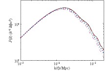 Figure1. (color online) The matter power spectrum
 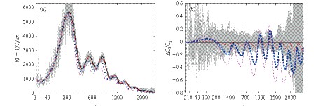 Figure2. (color online) The CMB temperature power spectra of (a)


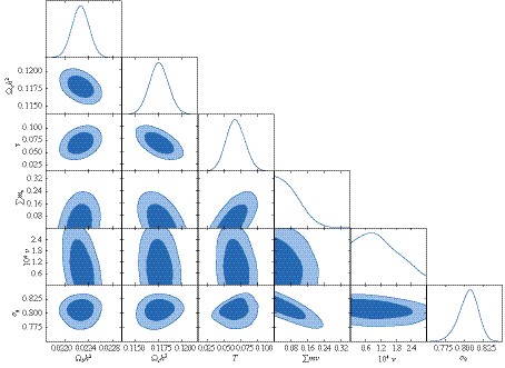 Figure3. (color online) One and two-dimensional distributions of


