 ,1,2, 李加林,1,3, 孙超1, 孙伟伟1, 曹罗丹1, 田鹏1
Classification of Yancheng coastal wetland vegetation based on vegetation phenological characteristics derived from Sentinel-2 time-series
LIU Ruiqing,1,2, LI Jialin,1,3, SUN Chao1, SUN Weiwei1, CAO Luodan1, TIAN Peng1通讯作者:
收稿日期:2020-09-10修回日期:2021-03-26网络出版日期:2021-07-25
| 基金资助: |
Received:2020-09-10Revised:2021-03-26Online:2021-07-25
| Fund supported: |
作者简介 About authors
刘瑞清(1995-), 女, 山西忻州人, 博士生, 研究方向为海岸海洋资源利用与保护。E-mail:

摘要
关键词:
Abstract
Keywords:
PDF (3735KB)元数据多维度评价相关文章导出EndNote|Ris|Bibtex收藏本文
本文引用格式
刘瑞清, 李加林, 孙超, 孙伟伟, 曹罗丹, 田鹏. 基于Sentinel-2遥感时间序列植被物候特征的盐城滨海湿地植被分类. 地理学报[J], 2021, 76(7): 1680-1692 doi:10.11821/dlxb202107008
LIU Ruiqing, LI Jialin, SUN Chao, SUN Weiwei, CAO Luodan, TIAN Peng.
1 引言
滨海湿地位于连接淡水河流系统与咸水海洋系统的沿海地带,是陆地和海洋生态系统之间的缓冲区[1],是地球上具有高生态经济价值以及潜在价值的独特生态系统[2],同时也是全球气候变化与人类活动共同作用下的生态敏感区域[3]。滨海湿地植被具有风暴防护、维持岸线稳定、防洪减灾、污染净化、营养循环、固碳以及栖息地保护等生态功能[4,5],是滨海湿地生态价值的主要维系,也是滨海湿地分布的重要参照[6]。国际地圈—生物圈计划(IGBP)的海岸带海陆相互作用研究(LOICZ)已将滨海湿地植被作为重要的研究对象,旨在推进海岸带可持续发展[7]。近百年来,全球气候变化以及人类干扰的巨大压力导致全球滨海湿地快速减少[8]。自20世纪70年代以来,中国沿海地区经济社会发展迅速,滨海湿地在人类过度开发活动的背景下面临严重退化风险[9,10]。为防止海岸侵蚀,实现保滩促淤[11],中国先后引入大米草和互花米草。米草植被在滨海湿地迅速扩张,与其他本地滨海湿地植被存在生态位竞争,对滨海湿地景观格局产生深远影响[12,13,14]。同时,为解决沿海地区的用地矛盾,中国海岸带地区进行了大规模的湿地围垦工程[15],造成了滨海湿地的大量消失[16]。因此,实现大区域滨海湿地长期精准监测对于沿海地区资源利用与生态保护至关重要。地物分布信息准确、及时获取是遥感领域面临的重要问题,滨海湿地植被向来是遥感监测的困难区域。一方面,滨海湿地植被分布范围广、群落组成复杂、光谱相似度高,造成了基于单一时相、中等空间分辨率影像的分类效果不佳;另一方面,高空间/高光谱遥感影像虽能取得较好的分类效果,但受限于数据成本和覆盖范围,上述影像难以应用在长时期、大范围的动态监测中[17,18,19,20]。已有研究表明不同植被的物候特征变化趋势存在明显差异[21],因此,本文考虑构建影像时间序列体现植被物候特征,以期提供一种顾及识别精度和监测广度的滨海湿地植被分类方法[19-20, 22-24]。随着遥感数据源日益丰富,数据获取性逐步提高,构建精细的年内影像时间序列数据得以实现,为植被变化动态监测带来可能。欧洲航天局(ESA)于2015年、2017年陆续发射2颗哨兵2号卫星(Sentinel-2 A/B),数据具备较高的时间分辨率(5 d)和空间分辨率(10 m),既为高分辨率影像时间序列滨海湿地植被识别创造了契机[25,26],又可细化滨海湿地观测的时间尺度,扩充海岸带遥感监测技术与方法体系。近年来Sentinel-2数据在滨海湿地信息提取监测技术方面已有相关研究,多数为滨海湿地中红树林、互花米草等植被分布的监测。当前滨海湿地遥感分类方法主要包括光谱、纹理、植被指数等单一特征或多特征变量分类法[26,27]、多源影像自动提取法[28]以及影像时间序列分类法[29]等。其中,遥感时间序列与植被物候信息相结合的分类方法研究[30]尚处于探索阶段,多数研究侧重于时间序列重建与植被物候变量提取,缺乏对植被物候特征信息可分性的深入挖掘。
基于此,本文以自然滨海湿地植被演替为主的盐城湿地作为研究区,以Sentinel-2影像为数据源,提出像元级SAVI时间序列及双Logistic植被物候特征拟合重构分类方法,有效避免云及云阴影干扰,在提高像元可用性的同时凸显滨海湿地植被物候特征差异,挖掘植被判别物候特征变量信息在植被快速精准提取方面的能力;分析滨海湿地植被精细识别方法的适用性,探讨大区域滨海湿地植被监测的可能,以期为海岸带资源开发与生态保护提供技术支持,助力海岸带经济与环境的统筹持续发展。
2 研究区概况与数据
2.1 江苏盐城湿地
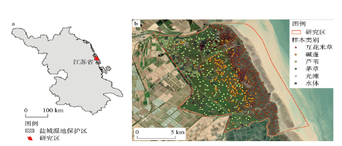
盐城滨海湿地(120°30′E~120°43′E, 33°28′~33°38′N),位于江苏省盐城市。盐城东缘直达黄海,南接南通、泰州两市,西与扬州、淮安相邻,北至连云港。本文选取盐城湿地珍禽国家级自然保护区的核心区——丹顶鹤保护区作为主要研究区(图1),该核心区地处江苏中部沿海射阳县的新洋港口到大丰县的斗龙港口之间的海岸段,西靠海堤,东为泥滩边缘,直面黄海(图1),位于典型的潮间带泥滩海岸之上,沿海岸湿地面积达19100 hm2,属于完全开敞型滨海湿地。盐城湿地原有景观为本地盐沼类型,植被种类匮乏,以耐盐植物为主,湿地优势植被群落为芦苇、茅草、碱蓬等,且具有典型的向陆演替规律。自20世纪中叶,人为引种外来植被的扩张使得盐城湿地植被类型及分布发生显著改变。互花米草作为外来物种,与本地的碱蓬植被生态位接近但其适应更低潮位,因而在海陆交界的潮滩上迅速扩张,近年来已严重影响本地种的生长演替。当前,盐城湿地仍在不断淤积扩张,形成新的潮滩与滨海湿地植被群落。图1
 新窗口打开|下载原图ZIP|生成PPT
图1盐城湿地区位及样本分布
Fig. 1Location and sample distribution of Yancheng wetland
2.2 遥感数据及预处理
本文选取盐城湿地2018年全年可获取的68景Sentinel-2 L1C级影像作为基础数据,影像标识号为T51STT。数据从欧空局数据中心网站(https://scihub.copernicus.eu)免费获取,投影为UTM 51N/WGS1984。Sentinel-2由A与B两颗卫星组成,重访周期为5天,其上的MSI多光谱成像仪覆盖13个,包括可见光谱、近红外和短波红外光谱。本文使用空间分辨率10 m的光谱波段,包括红、绿、蓝光和近红外波段。数据已完成辐射校正和几何校正,还需经过大气校正与影像掩膜处理。影像采用Sen2Cor插件进行大气校正,生成L2A级数据,然后参照SCL质量评估图像过滤云、卷云、云阴影覆盖像元,获取每景影像的可用像元。
2.3 滨海湿地覆被类型划分
经实地观测统计,盐城植被类型主要包括互花米草、碱蓬、芦苇、茅草等优势植被类型。本文结合实地调查采样及影像判读,参考当前盐城湿地分类结果,将研究区湿地划分为6类,分别为芦苇(Phragmites australis, PA)、碱蓬(Suaeda salsa, SS)、互花米草(Spartina alterniflora, SA)、茅草(Imperata cylindrica, IC)、光滩和水域。本文的重点在于滨海湿地植被的分类方法研究①(①为生成研究区完整分类图,基于植被指数SAVI数值变化特征对水域、光滩等地物加以区分。)。2.4 湿地样本数据
样本数据的获取方式主要包括2类,实地调查采样获取样方数据以及结合样方数据通过人为目视解译判读Google Earth高分影像获得。实地调查、采样点及样本数据分布见图1。本文共获取样本像元共694个,其中互花米草像元185个,碱蓬像元178个,芦苇像元208个,茅草像元45个,光滩像元25个,水域像元53个,用于时间序列模型筛选以及滨海湿地植被分类验证过程。3 研究方法
在模型构建前,综合考虑水体、土壤、植被等环境要素,选取了不同典型植被指数以及时间序列重构模型分别进行地物可分离性实验对比,最终研究提出SAVI(Soil-adjusted Vegetation Index)与双Logistic函数(Double Logistic function, DL)拟合方法相结合的像元级时间序列重构拟合模型,并结合植被物候特征,采用随机森林算法进行盐城滨海湿地植被分类,并将分类结果与常规影像分类方法加以比较,分析该方法在滨海湿地分类中的适用性。3.1 像元级时间序列模型重构
本文选取SAVI遥感影像特征指数进行像元级原始时间序列构建。SAVI是土壤调节植被指数,在NDVI基础上提出,修正了NDVI对土壤背景的敏感性。L是随着植被密度而发生变化的参数,取值范围为0~1,当植被覆盖度很高时为0,很低时为1。对于湿地而言,L取0.5时消除土壤反射率效果较好[31,32]。SAVI计算公式如下:式中:
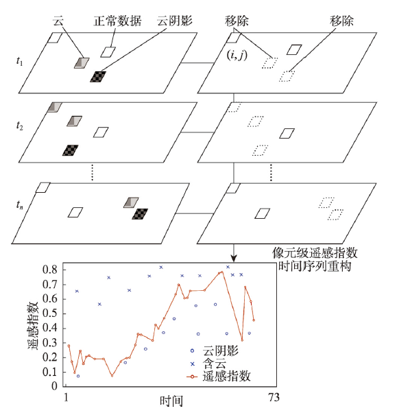
结合SAVI对经过预处理的每景Sentinel-2卫星遥感影像进行遥感指数计算。逐像元的SAVI原始时间序列是指在影像经掩膜处理后所有无云有效观测值形成的按时间顺序排列的遥感影像特征指数层的集合。如果用d代表时间序列t时刻的遥感影像特征指数值,通过提取图像中(i, j)处的像元值,则可生成一个连续的时间序列(ti, di)(图2),其中,i=1, 2, …, n。
图2
 新窗口打开|下载原图ZIP|生成PPT
图2逐像元的遥感影像特征指数原始时间序列示意图
Fig. 2Schematic diagram of the original time series of pixel-by-pixel image feature index
3.2 植被物候特征拟合模型构建
时间序列曲线会包含一定的“噪声”[33]。若直接采用原始时间序列进行地物分类研究,必然会影响滨海湿地分类总体精度,因此,需对时间序列影像数据质量进行改善。曲线函数拟合方法是基于原始时间序列,选用与植被物候生长规律相匹配的函数形式对时间序列曲线进行拟合,获得更为平滑、更符合植被物候生长规律的拟合曲线,适用于本文的数据环境与本文需求,可获取基于植被物候特征的曲线函数拟合模型。研究选取时间序列重构本文中广泛采用的双Logistic函数拟合方法应用于湿地分类。双Logistic拟合函数可用于时间序列拟合[34],采用分段局部拟合的方法[35],确定最终的双Logistic拟合曲线。其函数公式如下:其中,双Logistic函数的具体公式为:
式中:线性参数c1和c2确定用于曲线的基准面(对应植被的生长基准值)和振幅(对应季节性振幅)。在双Logistic函数中,x1和x3表示左侧(即生长季开始日期)和右侧(即生长季结束日期)的拐点位置,x2和x4决定了拐点的变化率(分别对应季初增长率、季末递减率)[36]。
3.3 基于植被物候特征的滨海湿地分类
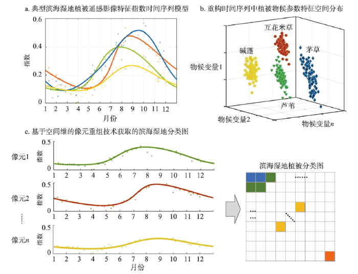
由于不同类型的湿地植被在时间序列模型上具有明显的形状分异(图3a),本文利用时间序列重构模型的物候特征参数构建特征空间,作为湿地精细分类的基础。具体而言,对于遥感影像特征指数,从时间序列模型中可以提取多个物候特征变量,由遥感影像特征指数衍生出的n维物候特征参数即可作为滨海湿地植被分类的特征空间(图3b)。本文主要选取季节开始时间、季节结束时间、基准值、季节性振幅、季初增长率与季末递减率6个物候特征变量完成湿地分类。通过选择典型训练样本,本文尝试随机森林机器学习分类算法确定各像元时间序列模型对应的湿地植被类型。在识别每一像元的湿地植被类型后,利用空间维的像元重组技术,最终获取观测时期内的滨海湿地分类图(图3c)。本文选取混淆矩阵[37]、Kappa系数[38]等评价指标用于分类结果精度验证。图3
 新窗口打开|下载原图ZIP|生成PPT
图3滨海湿地植被物候分类特征空间构建示意
Fig. 3Schematic diagram of spatial construction for phenological classification characteristics of coastal wetland vegetation
4 结果与分析
4.1 植被物候特征拟合曲线对比
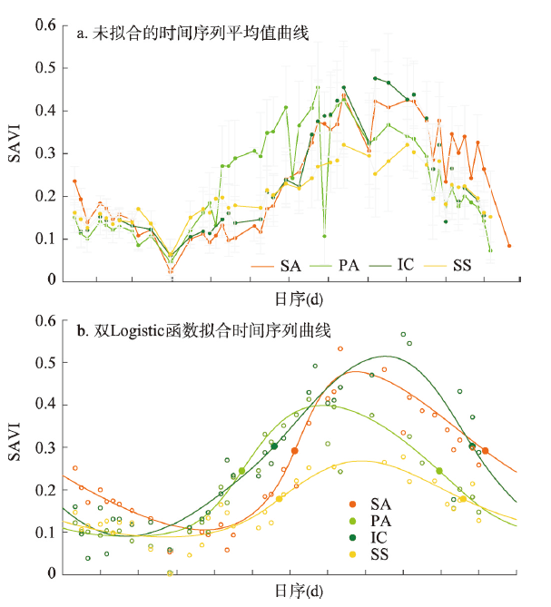
采用SAVI与双Logistic函数拟合时间序列重构模型获得盐城滨海湿地不同植被的拟合时间序列曲线,选取各植被类型代表样本像元的拟合曲线为研究对象,比较不同植被拟合曲线的物候特征提取效果(图4)。图4
 新窗口打开|下载原图ZIP|生成PPT
图4基于时间序列重构模型的盐城湿地各植被SAVI拟合曲线对比
Fig. 4Comparison of fitted curve of Yancheng wetland vegetation based on time series reconstruction model
相比于未拟合的SAVI时间序列,拟合曲线更为光滑,一定程度上消除了像元级时间序列影像数据中异常值“噪声”影响,更直观且准确地反映不同滨海湿地植被的物候变化规律。总体而言,芦苇、碱蓬、互花米草、茅草的物候变化趋势均为单峰变化,根据拟合曲线预估的生长季开始时间与结束时间可以得出,4类植被的生长旺盛期集中在5—12月,生长期峰值在7月末至10月间先后达到峰值,此后进入枯萎期,而在非生长季期间植被物候变化较为平缓。
对植被物候特征曲线进行分析,发现盐城滨海湿地不同植被类型间物候差异显著。芦苇的生长季开始时间最早,4月初开始生长,5月中旬进入生长旺盛期,7—8月达到峰值,9月进入生长后期,11月后完全枯萎。互花米草的生长旺盛期开始时间最晚,5月后曲线开始上升,季初增长率最大,7月初进入生长旺盛期,8—9月达到峰值,10月前后进入生长后期,12月进入枯萎期,1月后完全枯萎,枯萎期最晚。茅草的生长旺盛期开始于6月中旬,介于芦苇、互花米草之间,季初增长率略低于芦苇、互花米草,在9月中旬达到峰值,且峰值略高于互花米草;9月后开始快速衰败,季末递减率为最大,11月下旬生长季结束。碱蓬在4月开始生长,6—7月进入生长旺盛期,季初增长率最低,于8—9月间达到峰值,此后进入生长后期,10月开始逐渐枯萎,季末递减率较低,11月下旬生长季结束。
以上分析充分表明:植被物候特征拟合曲线能较为准确地反映不同滨海湿地植被类型的物候变化规律,也体现了本文基于时间序列重构方法下植被物候特征的分类方法对于滨海湿地分类具有很高的适用性。
4.2 植被物候特征提取及判别分析
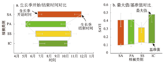
本文深一步探讨可用于各植被类型判别的有效物候特征参数,并针对不同植被类型划分物候特征参数阈值,为滨海湿地各植被类型的精准提取提供分类依据。对盐城滨海湿地不同植被的生长季时间与最值进行对比,如图5所示。从图5a中发现,芦苇的生长季开始时间明显早于其他植被,其他植被生长季开始时间集中于6月下旬至7月上旬,因此判别芦苇的植被物候特征参数阈值范围为:生长季开始时间5—6月。芦苇、碱蓬、茅草的生长季结束时间集中在10月中旬到11月初,而互花米草的生长季结束时间明显滞后于其他原生植被,结束时间在12月中旬前后,因此,判别互花米草的物候特征参数阈值范围为:生长季结束时间12月后期。从图5b中发现,互花米草与芦苇的基准值、峰值以及振幅大小基本相同,难以区分;碱蓬的基准值相对最大,峰值最小,振幅最小;茅草的基准值仅次于碱蓬,而其峰值最大,生长期振幅亦为最大。综上,判别碱蓬的植被物候特征参数阈值范围为:峰值0.25~0.35,振幅< 0.25。虽然茅草的SAVI峰值总体上超过芦苇与互花米草,但结合峰值的波动范围以及实地采样结果,茅草、芦苇与互花米草的峰值大小相似,峰值范围重叠较多,因此峰值不能作为茅草的物候特征判别参数。但结合基准值辅助分析,茅草的振幅显然超过其他植被类型,因此,判别茅草可选植被物候特征参数阈值范围为:振幅> 0.35,但此参数不能作为断定茅草植被类型的唯一参数。
图5
 新窗口打开|下载原图ZIP|生成PPT
图5基于时间序列重构模型的盐城湿地各植被生长季时间/最值对比
Fig. 5Comparison of growth season time/extremum of Yancheng wetland vegetation based on time series reconstruction model
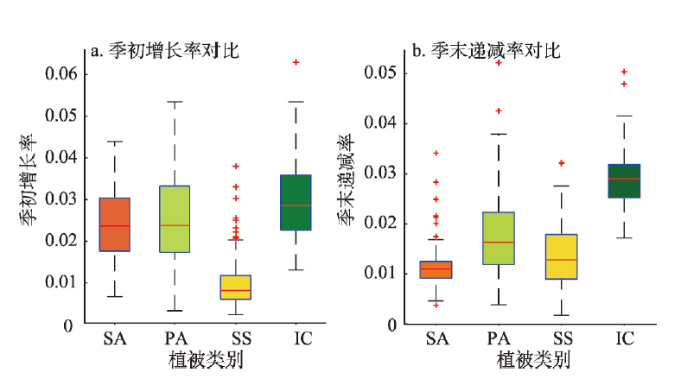
本文对盐城滨海湿地不同植被的生长期季初增长率与季末递减率进行对比看出(图6),芦苇与互花米草的季初增长率数据的中位数基本一致,茅草的季初增长率最高,而碱蓬的季初增长率明显低于其他植被,且其数据分布最为集中。因此,从各植被季初增长率数据的集中状况考虑,本文认为判别碱蓬的植被物候特征参数阈值范围为:季初增长率< 0.015。此外,由于茅草与芦苇、互花米草的季初增长率数据分布重叠较多,因此,茅草的季初增长率不能作为茅草的植被判别物候特征参数。从图6b中发现,互花米草的季末递减率最低,且季末递减率数据分布最为集中,碱蓬次之,其次是芦苇,茅草的季末递减率最大,数据分布较为集中,与其他植被的季末递减率数据总体分布重叠较少,因此,本文认为判别茅草的植被物候特征参数阈值范围为:季末递减率> 0.025。互花米草的季末递减率虽为最低,但其与碱蓬的季末递减率数据分布重叠较多,不具备判别互花米草的能力。
图6
 新窗口打开|下载原图ZIP|生成PPT
图6基于时间序列重构模型的盐城湿地植被增长率/递减率
Fig. 6Growth/decreasing rate of Yancheng wetland vegetation based on time series reconstruction model
综上,生长季开始时间(5—6月)可判别芦苇,生长季结束时间(12月后期)可判别互花米草,季末递减率(> 0.025)、振幅(> 0.35)为辅助可判别茅草,振幅(< 0.25)与季初增长率 (< 0.015)可判别碱蓬。遥感影像数据受水汽、云覆盖等因素影响往往存在数据不足或缺失、可用数据分布不均问题,且由于在植被生长旺盛期(通常为7—8月)进行滨海湿地分类精度最高,但在这一阶段滨海湿地会出现持续云雨天气,影像被水汽、云与云阴影遮挡,无法获得可用像元。通过构建植被物候特征参数用于滨海湿地分类能够一定程度规避数据不足及缺失、可用像元分布不均等问题,采用较少的可用像元数据即可构建基于植被物候特征的重构时间序列分类体系,因此,本文提出的分类方法在滨海湿地分类监测中具有很好的应用前景。此外,植被判别物候特征参数及阈值可为数据不足情况下的滨海湿地分类提供不同植被的判别依据,从植被物候特征角度实现不同植被的精准判别。
4.3 分类结果分析
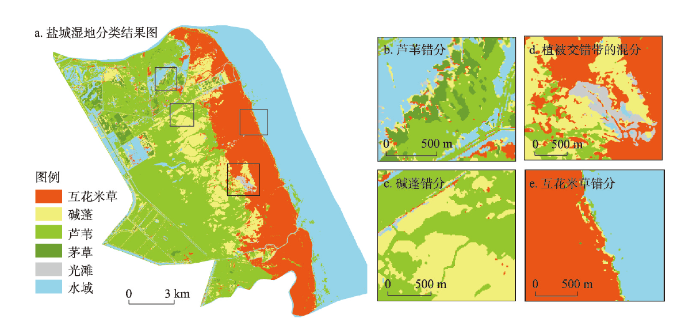
基于SAVI与双Logistic时间序列重构模型,对像元级物候特征变量数据进行随机森林分类,获得盐城滨海湿地分类图(图7),并采用分类混淆矩阵对分类结果进行评价(表1)。从表1发现,分类总体精度达到87.61%,而Kappa系数达到0.8358,盐城滨海湿地在基于植被物候特征分类方法下的分类精度总体较高。各湿地地物类型的使用者精度较高,均超过82%,表明分类中的错分误差相对较小。互花米草的使用者精度最高,其次是水域和芦苇,光滩和碱蓬次之,茅草的使用者精度最低。图7
 新窗口打开|下载原图ZIP|生成PPT
图7基于时间序列重构及植被物候特征分类方法的盐城湿地分类
Fig. 7Yancheng wetland classification map based on time series reconstruction and vegetation phenology feature classification
Tab. 1
表1
表1基于植被物候特征的滨海湿地分类精度评价结果
Tab. 1
| 互花米草 | 碱蓬 | 芦苇 | 茅草 | 光滩 | 水域 | 使用者精度(%) | |
|---|---|---|---|---|---|---|---|
| 互花米草 | 87 | 3 | 0 | 1 | 0 | 2 | 93.55 |
| 碱蓬 | 4 | 76 | 6 | 0 | 4 | 1 | 83.52 |
| 芦苇 | 1 | 9 | 96 | 2 | 0 | 3 | 86.49 |
| 茅草 | 1 | 1 | 1 | 19 | 1 | 0 | 82.61 |
| 光滩 | 0 | 1 | 0 | 0 | 6 | 0 | 85.71 |
| 水域 | 0 | 0 | 1 | 0 | 1 | 20 | 90.91 |
| 生产者精度(%) | 93.55 | 84.44 | 92.31 | 86.36 | 50.00 | 76.9 |
新窗口打开|下载CSV
结合盐城湿地分类结果及前期调研资料来看,分类图较好地展现了滨海湿地的植被空间分布状况,基本符合滨海湿地不同植被类型的生态位分布。由于核心区禁止围垦养殖,因此原先的围垦养殖塘已总体上恢复为自然湿地植被覆被。研究区内滨海湿地植被从陆到海呈群落条带状分布特征,在群落衔接地带由于优势植被生态位有所重叠而存在植被交错混合生长区域,植被群落的分布呈明显的破碎化分布。
在湿地植被交错带以及植被与水域、光滩相接地带容易出现错分现象(图7b~7e)。茅草的使用者精度偏低客观上是由于选取的茅草样本点数量过少导致精度存在误差,其错分现象主因是在植被交错带存在混合像元。芦苇主要被错分为茅草、碱蓬(如图7b),错分为茅草是二者物候特征相似性较强所致;错分为碱蓬则是由于芦苇像元与周围的水体、光滩混合,导致近红外反射率偏低,碱蓬与芦苇的生长期时段一致,因此,导致芦苇表现出类似碱蓬的SAVI变化趋势。碱蓬的错分往往集中于植被群落交错带,植被的混生致使混合像元难以区分(图7c、7d)。互花米草主要错分为碱蓬,分析其原因:一是在互花米草与潮滩相接区域存在错分为碱蓬的现象(图7e),这是由于互花米草外围往往生长着植株密度较低的植被,形成与潮滩、水域等的混合像元,同时受潮位涨落影响,互花米草被淹没,造成拟合曲线值被低估;二是互花米草与碱蓬的生态位有所重叠导致相互竞争生存空间,这一过程往往导致二者间存在混分现象。
4.4 与常规影像分类的对比分析
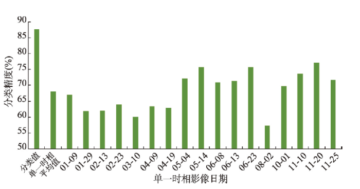
选取盐城滨海湿地研究区在2018年内所有成像清晰的单一时相影像,采用与本文相同的植被像元样本集,基于随机森林分类方法对每一景清晰影像进行分类,对各个单一影像分类与基于植被物候特征的分类进行盐城湿地分类的精度对比。最终得到各方法的总体精度(OA)(图8)。基于植被物候特征的分类方法总体精度为87.61%,而常规单一时相分类的总体精度均小于80%,总体精度的平均值为68.04%。从分类精度对比中可以发现,本方法的总体精度比常规的单一时相影像分类总体提高了19.57%。图8
 新窗口打开|下载原图ZIP|生成PPT
图8基于物候特征的分类与单一时相影像分类的总体分类精度对比
Fig. 8Comparison of overall classification accuracy between phenology-based classification and single temporal classification
此外,从单一时相影像分类精度对比中可以直观地发现,1—4月的影像分类精度普遍偏低,而从5月进入湿地植被生长期后,单景影像分类精度得到显著提升,其中5月14日、6月23日以及11月20日的影像分类精度较高,总体精度超过75%。由此证明,对于滨海湿地常规单影像分类而言,选择植被生长期的影像能显著提高分类精度。但湿地植被生长期往往与夏季多云雨天气对应,导致无法获取可用的植被旺盛期影像用于滨海湿地分类,如本文的7—9月Sentinel-2影像即使重访周期达5 d,但获取的影像均存在云覆盖问题,并无可用的清晰影像,这一现象导致滨海湿地分类存在数据不足或缺失等问题。这也是本文选取像元级影像用于分类的初衷,可以有效避免云及云阴影的干扰,增加影像像元信息的可用性。
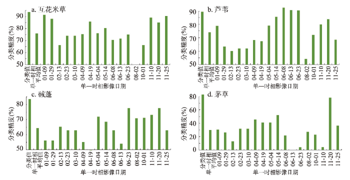
为进一步验证基于植被物候特征的分类方法对滨海湿地不同植被类型的判别分类效果,本文将2018年内各个单一时相影像分类与基于植被物候特征的分类进行不同湿地植被类型分类精度的对比,得到各类方法的不同滨海湿地植被类型分类精度对比图(图9)。
图9
 新窗口打开|下载原图ZIP|生成PPT
图9基于物候特征的分类与常规影像分类的不同植被分类精度对比
Fig. 9Comparison of classification accuracy (OA) of wetland vegetation between phenology-based classification and single temporal classification
从图9可以发现,基于物候特征的分类方法对盐城湿地各植被的分类精度均保持较高水平,而单一时相影像的分类往往能完成部分植被类型的提取,却很难保持不同植被类型分类的较高精度。因此,本文表明,基于物候特征的分类方法能够同时兼顾不同植被类型的分类准确性,在滨海湿地分类中具有很好的适用性。
其中,在单一时相影像分类中,互花米草在11月25日、1月9日的常规影像分类精度超过90%,充分表明生长季结束时间是互花米草的最佳判别物候期,这为实现互花米草的快速精准提取提供了新思路。同理,适合芦苇判别的较优单一影像分布时段主要集中在5—6月,芦苇的分类精度超过90%,表明生长季开始时间是芦苇的最佳判别物候期,该时段的影像可以实现芦苇植被的快速精准提取。值得注意的是,在单时相分类中芦苇的提取精度较植被物候特征分类更高,这进一步验证了常规光谱分类方法应用的前提是具有成像清晰的影像数据且分类对象为芦苇,而当易分类时段的影像质量较差或需提取滨海湿地各类植被时,植被物候特征分类方法的优势即可显现。碱蓬属于滨海湿地植被中较难区分的植被类型,仅通过单一时相影像分类较难实现碱蓬的精准判别,只有在采用植被物候特征分类方法时,才能较好地实现碱蓬的精准提取。11月中下旬(季末递减率)为判别茅草的最佳物候期。
5 结论
利用中高时空分辨率的Sentinel-2影像数据集,重构了像元级SAVI时间序列及双Logistic植被物候特征拟合模型,选取盐城滨海湿地为研究区进行随机森林分类,探讨了各植被类型判别的有效物候特征参数及阈值,分析了时间序列重构模型下基于植被物候特征的分类方法在滨海湿地分类中的优势及适用性。主要结论如下:(1)像元级SAVI时间序列拟合模型可准确提取盐城湿地不同植被的物候特征信息,反映植被物候变化规律。结果表明,盐城湿地各植被类型物候特征差异显著,芦苇生长期开始时间最早,互花米草生长季最晚,茅草SAVI值偏高,碱蓬物候期峰值最低。这为SAVI时间序列植被物候特征分类方法提供了依据。
(2)通过滨海湿地植被物候特征参数对比,植被判别物候特征参数及阈值可提供不同滨海湿地植被的判别依据,生长季开始时间5—6月、结束时间12月后期可分别判别芦苇、互花米草,季末递减率> 0.025、振幅> 0.35为辅助可判别茅草,振幅< 0.25与季初增长率< 0.015可判别碱蓬。物候参数的确定使得从植被物候特征角度实现植被精准判别的方法具备推广应用价值,可服务于滨海植被快速精准提取,也为解决滨海湿地分类研究中重要影像信息缺失或不足的问题提供了新思路。
(3)Sentinel-2像元级遥感时间序列植被物候特征分类方法下,盐城滨海湿地分类结果较好,总体精度达87.61%,相较于常规单时相影像分类方法总体精度有大幅提高,对不同湿地植被的精准判别优势较为显著,在滨海湿地分类监测领域具有很好的适用性。
基于时间序列植被物候特征的分类方法通过结合植被物候特征能实现滨海湿地植被群落混生带的精准分类以及对“异物同谱”植被的有效区分,有效提高滨海湿地分类精度,可提供较高分辨率的年际滨海湿地植被分布信息,服务于海岸带资源开发与湿地生态保护。未来应继续探讨本方法在其他区域滨海湿地植被分类中应用的可能性并推广使用。此外还可进一步探讨本方法在陆地卫星等其他遥感传感器中的适用性,服务于滨海湿地植被精细动态监测。
参考文献 原文顺序
文献年度倒序
文中引用次数倒序
被引期刊影响因子
URL [本文引用: 1]
DOI:10.1038/nclimate3203URL [本文引用: 1]
DOI:10.1038/nature12856URL [本文引用: 1]
DOI:10.1007/s11356-019-05352-2URL [本文引用: 1]
DOI:10.1016/j.ecoser.2014.06.010URL [本文引用: 1]
DOI:10.1890/10-1510.1URL [本文引用: 1]
DOI:10.1016/j.ecss.2007.09.016URL [本文引用: 1]
DOI:10.1146/annurev.marine.010908.163930URL [本文引用: 1]
DOI:10.1016/j.envint.2015.02.017URL [本文引用: 1]
[本文引用: 1]
[本文引用: 1]
DOI:10.1016/j.ecoleng.2005.09.012URL [本文引用: 1]
DOI:10.1016/j.ecoleng.2011.12.014URL [本文引用: 1]
DOI:10.1360/zd-2014-44-11-2339URL [本文引用: 1]
[本文引用: 1]
[本文引用: 1]
[本文引用: 1]
DOI:10.11821/dlxb202001010 [本文引用: 1]

The spatial pattern changes of bays under the influence of reclamation can profoundly reflect how human activities affect the natural environments, which is important to effectively protect and utilize bay resources. Based on 6 Landsat TM/OLI remote sensing images during 1990-2015, this study analyzed the variations of major bays from the coastline and bay surface morphology and explored the correlation between the reclamation intensity and spatial pattern changes for the 12 major bays in the East China Sea (ECS). The main conclusions include that: (1) the length of the main bay coastline in the East China Sea, from 1990 to 2015, increased by 66.65 km. The extensive coastline growth was found during 2005-2010 and the growth reached 38 km. Sansha Bay has the longest coastline (439 km) and the shortest (105 km) was found in Luoyuan Bay; Xinghua Bay experienced the largest coastline growth (54.53 km) in the past decades, and the least was in Luoyuan Bay (25.75 km). In general, the artificial coastline continued to increase and the degree of artificialization had been continuously strengthened. (2) The coastline of the bay continuously moved to the sea, with a distance of 26.93 km (1.08 km/a). The most significant seaward expansions were found in 1995-2000 and 2005-2010, reaching 7.10 km and 6.00 km, respectively. Hangzhou (4.93 km) and Xinghua bays (4.15 km) experienced the largest seaward expansion of coastline, while Xiamen Bay had the shortest (0.55 km). (3) The total area of the major bay waters decreased from 13.85 km2 in 1990 to 12.29 km2 in 2015 in the East China Sea, down by 11.23%. Additionally, the morphological indices of the bays showed a continuous rise trend, which indicates that spatial patterns were transformed to be more complicated. The largest reduction with water area was observed in the Hangzhou Bay (0.726 km2), accounting for 46.69% of the research area. (4) The indexes of artificiality and development intensity showed a continuous rise trend. The utilization degree in the southern part of the study area is higher than that of the northern part, and the interannual fluctuation of the development intensity in the north is much varied. In addition, the bay development is positively correlated with the length of the coastline, the length of the artificial coastline and the shape index of the bay, and negatively correlated with the length of the natural coastline and the area of the waters. As the development intensity increased, the intensity of reclamation activities increased significantly.
[本文引用: 1]
DOI:10.1007/s11442-020-1772-1URL [本文引用: 1]
DOI:10.1016/j.jenvman.2014.05.027URL [本文引用: 1]
DOI:10.1016/j.rse.2009.10.009URL [本文引用: 1]
DOI:10.1016/j.rse.2017.07.034URL [本文引用: 2]
DOI:10.1016/j.rse.2017.09.023URL [本文引用: 2]
DOI:10.1016/j.rse.2013.07.015URL [本文引用: 1]
DOI:10.1016/j.jag.2015.10.008URL [本文引用: 1]
[D].
[D].
DOI:10.1016/j.ecolind.2014.01.041URL [本文引用: 1]
DOI:S0301-4797(19)30899-0PMID:31336348 [本文引用: 1]
Although wetlands remain threatened by human pressures and climate change, monitoring and managing them are challenging due to their high spatial and temporal dynamics within a fine-grained pattern. New satellite time-series at high temporal and spatial resolutions provide a promising opportunity to map and monitor wetlands. The objective of this study was to develop an operational method for managing valley bottom wetlands based on available free remote sensing data. The Potential, Existing, Efficient Wetlands (PEEW) approach was adapted to remote sensing data to delineate three wetland components: (1) potential wetlands, mapped from a digital terrain model derived from LiDAR data; (2) existing wetlands, delineated from land cover maps derived from Sentinel-1/2 time-series; and (3) efficient wetlands, identified from functional indicators (i.e. annual primary production, vegetation phenology, seasonality of carbon flux) derived from MODIS annual time-series. Soil and vegetation samples were collected in the field to calibrate and validate classification of remote sensing data. The method was applied to a 113?000?ha watershed in northwestern France. Results show that potential wetlands were successfully delineated (82% overall accuracy) and covered 21% of the watershed area, while 44% of existing wetlands had been lost. Small wetlands along headwater channels, which are considered as ordinary, cover 56% of wetland area in the watershed. Efficient wetlands were identified as contiguous pixels with a similar temporal functional trajectory. This method, based on free remote sensing data, provides a new perspective for wetland management. The method can identify sites where restoration measures should be prioritized and enables better understanding and monitoring of the influence of management practices and climate on wetland functions.Copyright © 2019 Elsevier Ltd. All rights reserved.
[本文引用: 2]
[本文引用: 2]
DOI:10.3390/rs12091383URL [本文引用: 1]
[本文引用: 1]
[本文引用: 1]
[D].
[本文引用: 1]
[D].
[本文引用: 1]
DOI:10.3390/rs11212479URL [本文引用: 1]
DOI:10.1029/98JD00051URL [本文引用: 1]
DOI:10.1016/0034-4257(88)90106-XURL [本文引用: 1]
[D].
[本文引用: 1]
[D].
[本文引用: 1]
DOI:10.1016/j.rse.2005.10.021URL [本文引用: 1]
DOI:10.1016/j.rse.2013.01.011URL [本文引用: 1]
DOI:10.1016/j.rse.2007.01.004URL [本文引用: 1]
DOI:10.3964/j.issn.1000-0593(2019)07-2271-07 [本文引用: 1]
Hyperspectral imaging technology has been widely used in the detection of agricultural products. This paper studies the non-destructive identification of millet samples from different regions based on hyperspectral imaging and machine learning algorithms. The millet samples from seven provinces were divided into five categories according to geographical regions. They were Dongbei, Hebei, Shaanxi, Shandong, and Shanxi, respectively. A total of 23 samples were collected in these areas, including 6 samples in Dongbei, 5 samples in Shanxi, and respective 4 samples in Hebei, Shaanxi, and Shandong. Each sample was equally divided into 10 equal parts and the hyperspectral data of millet in the wavelength band from 900 to 1 700 nm was collected using a hyperspectral imager. In order to reduce the influence of uneven illumination and dark current on the experiment, the collected hyperspectral data was corrected in black and white. The ENVI software was used to select the region of interest (ROI) of millet hyperspectral image, and 9 ROIs were selected for each sample of millet. The average spectral value in the ROI was calculated, which was used as a spectrum record of the sample. Finally, a total of 2 070 spectral curves were collected, of which 540 from Dongbei, 450 from Shanxi, and several 360 from Hebei, Shandong, and Shaanxi respectively. In order to reduce the scattering phenomenon caused by the unevenness of the sample surface, which would affect the true spectral information of millet, the multivariate scatter correction (MSC) pretreatment was performed on the original spectrum. In addition, randomized division method was used to divide the corrected spectral data into training set and test set. The ratio of test set was 0. 3. Linear Discriminant Analysis (LDA) was used to visualize spectral data of millet from different origins. Substituting the test set into a well-trained LDA model, and finally a confusion matrix of prediction results was created. The results showed that LDA had a prediction accuracy of 0. 84 and 0. 99 for Shaanxi and Shanxi, and only 0. 68, 0. 68, and 0. 40 for Dongbei, Hebei, and Shandong. Therefore, the recursive feature elimination (RFE) was used to select useful spectral information, remove redundant information, and improve the prediction accuracy. The RFE combined with support vector machine (SVM) and Logistic Regression (LR) were used to compare and analyze the discriminant of millet from different regions. Substituting training set of millet spectral data into SVM-RFE and LR-RFE models, and the corresponding feature subsets were selected optimally by the micro-averaging of the model F-values and 3-fold cross validation technology. The results showed that the number of wavelengths selected by the LR-RFE was 74 and the Micro_F of the model was 0. 59 ; Meanwhile the number of wavelengths selected by the SVM-RFE was 220 and the Micro_F of the model was 0. 66. The selected feature subset was applied to the test set. Substituting the test set into SVM and LR models respectively, and confusion matrix of model prediction results and the receiver operating characteristic curve (ROC) of the model were used as the evaluation method. The results showed that the accuracy of SVM-RFE prediction was 1, 0. 37, 0. 72, 0, and 1 for Dongbei, Hebei, Shaanxi, Shandong, and Shanxi, and the area under ROC curve (AUC) was 0. 82, 0. 92, 0. 93, 0. 70, and 0. 99 respectively. The accuracy of LR-RFE prediction was 0. 92, 0, 0. 97, 0, and 0. 80, and the AUC was 0. 72, 0. 74, 0. 94, 0. 66, and 0. 88 respectively. It can be seen from the prediction results that the overall classification performance of SVM-RFE model was better than that of LR-RFE, while the discrimination of Shaanxi class LR-RFE was better than that of SVM-RFE. For the Hebei and Shandong categories, neither model could effectively discriminate it. Compared with LDA, the prediction accuracy of these two models had been improved.
[本文引用: 1]
[本文引用: 1]
[本文引用: 1]
