删除或更新信息，请邮件至freekaoyan#163.com(#换成@)

基于灰色关联模型对江苏省PM2.5浓度影响因素的分析

本站小编 Free考研考试/2021-12-29

贺祥¹^,²^,³^,, 林振山¹^,³^,, 刘会玉¹^,³, 齐相贞¹^,³

1. 南京师范大学地理科学学院,南京 210023

2. 凯里学院,凯里 556011

3. 江苏省地理信息资源开发与利用协同创新中心,南京 210023

Analysis of the driving factors of PM_2.5 in Jiangsu province based on grey correlation model

HEXiang¹^,²^,³^,, LINZhenshan¹^,³^,, LIUHuiyu¹^,³, QIXiangzhen¹^,³

1. College of Geography Science, Nanjing Normal University, Nanjing 210023, China

2. Kaili University, Kaili 556011, Guizhou, China

3. Jiangsu Center for Collaborative Innovation in Geographical Information Resource Development and Application, Nanjing 210023, China

通讯作者:林振山(1955-), 教授, 博士生导师, 主要从事人类活动环境效应研究。E-mail:linzhenshan@njnu.edu.cn
收稿日期:2016-02-25
修回日期:2016-03-21
网络出版日期:2016-07-25
版权声明:2016《地理学报》编辑部本文是开放获取期刊文献，在以下情况下可以自由使用：学术研究、学术交流、科研教学等，但不允许用于商业目的.
基金资助:

国家自然科学基金项目(31470519)

2015年江苏省高校自然科学研究重大项目(15KJA17002)

江苏省自然科学基金项目(BK20131399)

江苏省高校优势学科建设工程资助项目

贵州省科技厅基金项目([2014]7237)

贵州省教育厅人文社科项目(13GH004)

作者简介:
-->作者简介：贺祥(1978-), 男, 贵州水城人, 博士, 副教授, 主要从事生态与环境研究。E-mail:hexiang1997403@163.com

展开

摘要
采用克里金插值法分析2014年江苏省PM_2.5浓度空间分布特征,运用灰色关联模型计算PM_2.5浓度与影响因素间关联度,分析主要影响指标因子与PM_2.5浓度空间分布的相互关系。结果显示：① 江苏省PM_2.5浓度具有沿海低、内陆高,南部高、北部低的空间分布特征;② PM_2.5污染来源指标层的权重值最大（w_i = 0.4691）,空气质量与气象要素指标层的权重稍大（w_i = 0.2866）,城市化与产业结构层的权重值最小（w_i = 0.2453）;③ 在27个指标因子中,与PM_2.5浓度关联度为中度的仅有公路客运量、房屋建筑施工面积、园林绿地面积、人口密度等4个指标因子,PM_2.5与其余指标因子均呈强度相关联,其中与PM₁₀、O₃、降雨量、公路货运总量、地区工业总产值和第二产业占地区生产总值比重等指标的关联度较高;④ PM_2.5污染源指标层与PM_2.5浓度关联度值较大的城市分别是南京、无锡、常州、南通、泰州市;城市化与产业结构指标层与PM_2.5浓度关联度值较大的城市分别是徐州、苏州、盐城、常州市;空气质量与气象要素指标层与PM_2.5浓度关联度值较大的城市分别是盐城、扬州、常州、南通市。综合分析可知,影响指标因子关联度值与PM_2.5浓度空间分布有较好相关性。研究表明,灰色关联模型可有效分析影响PM_2.5浓度的主要因素,能对PM_2.5浓度影响指标进行定量分析与评价。

关键词：灰色关联模型;PM2.5浓度空间分布;影响指标因子;江苏省
Abstract
In this paper, the Kriging interpolation method was introduced to analyze the spatial distribution characteristics of PM_2.5 in Jiangsu province in 2014, and then the evaluation index system for the PM_2.5 was constructed, which consists of three index layers and 27 indexes. The grey correlation analysis method was used to explore the correlation between PM_2.5 and its influencing factors. Finally, the relationship between the spatial distribution of PM_2.5 and the main influencing factors was analyzed. The conclusions can be drawn as follows: (1) The PM_2.5 in the coastal areas and the north is lower, while it is higher in the inland areas and the south. (2) The weight of PM_2.5 pollution sources index layer is the largest (w_i = 0.4691), the weight of the air quality index and meteorological elements layer is larger (w_i = 0.2866), and the weight value of urbanization and industrial structure index layer is the minimum (w_i = 0.2453). (3) In the 27 indexes, the volume of highway freight, housing construction area, garden green space area and population density have moderate correlation degrees. The other indexes have strong correlation degrees, among which, the correlation degree of the PM₁₀, O₃, total road freight volume and gross industrial output value are relatively high. (4) The synthetic correlation degree values between the PM_2.5 pollution sources index layer and PM_2.5 are much higher in cities of Nanjing, Wuxi, Changzhou, Nantong and Taizhou. The synthetic correlation degree values between urbanization and industrial structure index layer and PM_2.5 are much higher in cities of Xuzhou, Suzhou, Yancheng and Changzhou. The synthetic correlation degree values between the air quality index and meteorological elements layer and PM_2.5 are much higher in cities of Yancheng, Yangzhou, Changzhou and Nantong. Our results demonstrate that the grey correlation degrees of the evaluation indexes system are closely related with spatial distribution of PM_2.5 in Jiangsu province. Therefore, the grey correlation analysis model can be employed to analyze and evaluate the spatial distribution of PM_2.5.

Keywords：grey correlation model;the spatial distribution of PM2.5;influencing index;Jiangsu province

-->0
PDF (1683KB)元数据多维度评价相关文章收藏文章
本文引用格式导出EndNote Ris Bibtex 收藏本文-->
贺祥, 林振山, 刘会玉, 齐相贞. 基于灰色关联模型对江苏省PM_2.5浓度影响因素的分析[J]. , 2016, 71(7): 1119-1129 https://doi.org/10.11821/dlxb201607003
HE Xiang, LIN Zhenshan, LIU Huiyu, QI Xiangzhen. Analysis of the driving factors of PM_2.5 in Jiangsu province based on grey correlation model[J]. 地理学报, 2016, 71(7): 1119-1129 https://doi.org/10.11821/dlxb201607003

1 引言

PM_2.5对环境、人体健康及社会经济发展产生重要影响,国内外****对它进行了大量研究,主要包括对PM_2.5的跨界扩散与传输^[1],PM_2.5污染特征及其影响因素^[2-4],PM_2.5污染物组成及其来源解析^[5-7],PM_2.5对人体健康的影响^[8-11],PM_2.5受气象、环境因素影响^[12-13],以及PM_2.5排放来源及排放源清单^[14-16]等方面的研究。针对PM_2.5影响因素的研究,钟无涯等^[17]从城市生活、生产方式与区域产业结构转型3个不同层面探讨与PM_2.5的关系,认为区域产业结构转型、升级和生产方式转变是改善PM_2.5问题途径之一;齐园等^[18]对北京3次产业演变与PM_2.5排放的动态关系进行研究,认为第二产业是PM_2.5排放的长期主要来源,机动车辆及餐饮业是PM_2.5的重要来源;莫莉等^[19]研究认为城市化程度与PM_2.5等颗粒物浓度有明显的关系,与地区生产总值呈正相关,与林木覆盖率呈负相关;Pateraki等^[20]将风速、气温、相对温度及天气条件等因素考虑到PM_2.5浓度形成研究中,并得到气象条件对PM_2.5形成具有显著影响的结论;Yang等^[21]还通过大气稳定气流、气温等因素去研究PM_2.5形成条件及极端雾霾的产生条件与过程。针对PM_2.5污染时空变化影响因素的研究,Querol等^[22]对西班牙1999-2005年PM_2.5的时空变化及影响因素进行了探究,认为气象因素具有显著影响作用;Zheng等^[23]通过有机碳、碳气溶胶和硫酸盐、硝酸盐和铵等主要离子对比分析中国与美国PM_2.5浓度季节变化特征;Xie等^[24]对中国31省份分析认为SO₂、NO₂、CO和O₃等与PM_2.5浓度空间分布存在显著相关性;王占山等^[25]对北京市35个监测站PM_2.5数据分析其时空分布特征及与前体物和大气氧化性的相关性关系。一些****还运用土地利用回归（LUR）模型方法研究不同土地利用类型要素对PM_2.5空间分布特征的影响^[26-30]。虽然许多****对PM_2.5浓度变化与时空分布的影响因素进行了大量研究,但多数****仅考虑了部分指标因素,很少****基于气象、污染源和社会经济等因素的综合影响进行研究。
PM_2.5的形成是大气环境是一个非常复杂系统过程,污染源多样性显著,其中既包含大量已知又含有未知的信息状态,所以它也是一个灰色系统。因此,本研究将采用灰色关联模型方法对江苏省13个省辖市PM_2.5浓度影响指标因子进行综合研究。具体方法与步聚是：首先,对江苏省各省辖市PM_2.5浓度时空分布进行分析,构建PM_2.5浓度影响因素指标体系,包括空气质量指标、气象要素、城市化、工业排放废气、交通尾气、建筑扬尘等3个层次的27个指标因素;其次,利用灰色关联法对PM_2.5浓度与影响指标因子间关联程度进行分析,计算3个指标层次与PM_2.5浓度间的关联度,得到各指标因子的关联度排序;最后分析主要影响指标因子与PM_2.5浓度空间分布的关系。

2 研究方法与PM_2.5浓度影响指标数据

2.1 研究方法

2.1.1 熵值法确定权重系数在信息论中,熵值反映了信息的无序化程度,可以用来度量信息量的大小,某项指标携带的信息越多,表示该指标对决策的作用越大^[31]。熵值法的计算步骤如下：
（1）构建m个方案,n个评价指标的判断矩阵：

\begin{matrix} X = (\begin{matrix} x_{11} & x_{12} & \begin{matrix} ? & x_{1 n} \end{matrix} \\ \begin{matrix} x_{21} \\ ? \end{matrix} & \begin{matrix} x_{22} \\ ? \end{matrix} & \begin{matrix} \begin{matrix} ? & x_{2 n} \end{matrix} \\ \begin{matrix} ? & ? \end{matrix} \end{matrix} \\ x_{m 1} & {x_{m}}_{2} & \begin{matrix} ? & x_{mn} \end{matrix} \end{matrix}), X = {x_{ij}}_{m \times n}, (i = 1, 2, \dots m; j = 1, 2, \dots n) \end{matrix}

（1）
（2）数据的无量纲处理,对原始数据需要消除量纲,进行标准化处理,转换为可比较数据序列。
（3）根据熵的定义,m个评价事物n个评价指标,可以确定评价指标的熵为：

\begin{matrix} f_{ij} = \frac{{x_{i}}_{j}}{\overset{n}{\sum_{j = 1}} {x_{i}}_{j}}, (j = 1, 2, \dots, n) \end{matrix}

（2）

\begin{matrix} e_{j} = - \frac{1}{lnm} \overset{n}{\sum_{i = 1}} f_{ij} \ln f_{ij} \end{matrix}

（3）
式中：e_j为第j个指标的熵;f_ij为第i个评价对象第j个评价指标标准值的比重;如果f_ij = 0,则定义f_ijlnf_ij = 0。那么第j项指标的熵权即可以定义为：

\begin{matrix} w_{j} = \frac{1 - e_{j}}{\overset{n}{\sum_{j}} (1 - e_{j})}, (w_{j} \in [0, 1], \overset{n}{\sum_{j = 1}} w_{j} = 1) \end{matrix}

（4）
2.1.2 灰色关联分析法根据Deng^[32]、刘思峰等^[33]提出的灰色关联公理及计算公式,具体步骤如下：
（1）确定特征序列和因素序列：
进行灰色关联分析,首先要确定作为参照的特征序列和被比较的因素序列。记特征序列为x₀(t),共采集m个数据,即：x₀(t)={x₀(1), x₀(2),…, x₀(m)},t =1, 2, …m;记因素序列为x_i(t),其中有n个子序列,即：x_i(t)={x_i(1), x_i (2),…, x_i (m)},i =1, 2, …n。
（2）如果系统中各因素的量纲不相同,数据无法直接比较,则需要进行标准化处理。
（3）求关联系数和关联度：
① 计算关联系数：

\begin{matrix} ξ (x_{0} (t), x_{i} (t)) = \frac{\min_{i} \min_{t} |x_{0} (t) - x_{i} (t)| + ρ \max_{i} \max_{t} |x_{0} (t) - x_{i} (t)|}{|x_{0} (t) - x_{i} (t)| + ρ \max_{i} \max_{t} |x_{0} (t) - x_{i} (t)|} \end{matrix}

（5）
式中：

\begin{matrix} \min_{i} \min_{t} |x_{0} (t) - x_{i} (t)| \end{matrix}

、

\begin{matrix} \max_{i} \max_{t} |x_{0} (t) - x_{i} (t)| \end{matrix}

分别为极差最小值和极差最大值;ρ为分辨率,一般取值为0.5。
② 计算加权关联度：

\begin{matrix} {R_{i}}_{j} = \overset{n}{\sum_{i = 1}} w_{j} \times ξ_{i} (x_{0} (t), x_{i} (t)) \end{matrix}

（6）

2.2 PM_2.5浓度影响指标体系与数据来源

2.2.1 PM_2.5浓度影响指标体系构建 PM_2.5主要来源为二次硝酸盐和硫酸盐、煤燃烧、机动车尾气（尘）、道路扬尘、土壤扬尘、建筑尘、生物质燃烧等,其形成与变化还受气象等多因素影响。因此,依据其组成来源及影响因素,构建3个指标层,包含27个指标因子的影响指标体系（表1）：① 空气质量指标与气象要素指标层,包括PM₁₀、SO₂、平均风速、平均气温、平均降雨量和平均相对湿度等10个指标因子,反映空气污染物在一定气象条件下形成PM_2.5的程度;② PM_2.5污染物来源指标层：工业生产,以工业用电量指标表征工业生产过程燃煤、工业尾气排放量;工业废气排放,包括二氧化硫排放量,氮氧化物排放量,烟（粉）尘排放量,表征大气污染废气量;交通与路网,主要以等级公路里程、公路客运量、公路货运总量、机动车保有量,表征交通运输排放废气量;建筑,以房屋建筑施工面积为指标因子,主要表征建筑扬尘量;③ 城市化与社会产业指标层：净化空气能力指标,包括园林绿地面积、建成区绿地覆盖率、人均公园绿地面积,反映城市绿化对降低PM_2.5污染的能力;人口密度和市区建成面积指标因子,反映城市建设对PM_2.5浓度的影响;产业结构,反映城市社会产业结构对PM_2.5污染物排放量的影响,包括第二产业占地区生产总值比重、人均地区生产总产值与市区工业总产值等指标因子。
2.2.2 数据来源 PM_2.5数据及空气质量指标数据来源于中国环境监测总站（http://www.cnemc.cn/）,包括PM_2.5、PM₁₀、NO₂、O₃、SO₂和CO等6个空气质量监测指标。研究数据是由江苏省13个省辖市内所有监测站的每日平均值计算得到。气象数据来源于中国气象数据网（http://data.cma.cn/）,主要包括日平均气温、平均相对湿度、平均降水量、平均风速和日照时数等5个指标因子。PM_2.5污染物来源及城市化与社会产业指标因子数据来源于《2015年江苏统计年鉴》与2014年江苏省国民经济和社会发展统计公报（表2）。
Tab. 1
表1
表1江苏省PM_2.5浓度的影响指标体系
Tab. 1PM_2.5 influencing index system in Jiangsu province

指标层		指标因子	指标层		因素层	指标层		指标因子
空气质量指标与气象要素	大气污染物	PM₁₀(μg/m³) (X₁)	PM_2.5污染来源	交通	等级公路里程(km) (X₁₁)	城市化与产业结构	城市与绿化面积	园林绿地面积*(hm²) (X₂₀)
		SO₂(μg/m³）（X₂）			公路客运量(万人)(X₁₂)			建成区绿地覆盖率*(%)(X₂₁)
		CO (mg/m³)(X₃)			公路货运总量(10 kt) (X₁₃)			人均公园绿地面积* (m²/人) (X₂₂)
		NO₂(μg/m³) (X₄)			机动车保有量(万辆)(X₁₄)			建成区面积(km²)(X₂₃)
		O₃* (μg/m³) （X₅）		工业生产	工业用电量(亿千瓦时)(X₁₅)		人口数量	人口密度(人/km²)(X₂₄)
	气象要素	降水量*(0.1mm) (X₆)		工业废气排放	二氧化硫排放量(t) (X₁₆)		产业结构	第二产业占地区生产总值比重(X₂₅)
		平均风速*(0.1m/s) (X₇)	氮氧化物排放量(t) (X₁₇)			人均地区生产总产值(元) (X₂₆)
		平均气温(0.1℃) (X₈)	烟(粉)尘排放量(t) (X₁₈)			地区工业总产值(亿元)(X₂₇)
		平均相对湿度(1%) (X₉)	建筑		房屋建筑施工面积(10 km²) (X₁₉)	–	–	–
		日照时数 (0.1 h) (X₁₀)		–	–	–	–	–

注：*表示负向型指标,其余为正向型指标。

新窗口打开
Tab. 2
表2
表2江苏省13个省辖市PM_2.5浓度影响指标因子的数据
Tab. 2Data of the PM_2.5 influencing indices for the 13 provincial cities in Jiangsu province

指标层		因子	南京市	无锡市	徐州市	常州市	苏州市	南通市	连云港市	淮安市	盐城市	扬州市	镇江市	泰州市	宿迁市
PM_2.5		X₀	73.82	67.27	67.28	66.48	65.92	61.51	74.78	68.65	58.30	65.93	67.28	62.83	68.81
空气质量指标及气象要素	大气污染物	X₁	123.46	105.38	118.86	103.76	89.98	93.89	112.03	101.78	92.54	112.29	109.70	110.42	114.88
		X₂	23.00	28.17	37.95	35.16	22.06	26.37	29.68	27.66	19.83	33.06	24.40	30.61	27.11
		X₃	0.90	1.10	1.22	1.10	0.93	0.74	1.01	1.07	0.77	0.83	1.18	1.21	1.20
		X₄	50.82	44.28	37.16	44.57	51.79	36.30	35.28	23.33	25.43	32.22	45.33	22.87	33.18
		X₅	99.43	101.66	91.68	102.48	95.89	105.04	98.83	111.73	101.12	86.79	90.05	75.59	92.01
	气象要素	X₆	29.99	37.99	22.76	33.21	34.84	36.43	23.55	26.92	37.48	30.56	23.50	22.84	28.74
		X₇	25.96	22.01	17.31	20.93	20.76	28.67	20.03	21.39	22.81	18.76	28.08	22.64	17.30
		X₈	165.09	168.78	156.64	157.37	171.46	159.49	147.39	149.43	149.53	163.13	158.22	156.89	150.55
		X₉	73.96	73.36	66.08	66.12	73.61	77.40	75.31	77.32	78.60	72.47	86.75	74.52	73.01
		X₁₀	51.06	47.23	60.83	48.84	44.47	50.00	53.19	47.15	60.08	56.23	58.86	57.60	54.14
PM_2.5 污染物来源	交通	X₁₁	11131	2951	3926	4276	4610	3928. 0	1529	4871	2891	4203	1602	3242	3228
		X₁₂	10493	3364	10259	4673	24010	6586	3133	4420	4018	6035	2245	3437	1374
		X₁₃	10912	4734	7529	6932	5065	4769	3053	2220	2110	6155	3529	1123	762
		X₁₄	140.41	67.63	35.80	61.01	113.22	34.56	12.13	19.30	14.91	29.02	16.15	17.97	14.45
	工业生产	X₁₅	286.71	194.01	158.90	215.48	418.01	96.62	28.35	63.65	24.96	69.70	84.67	53.43	51.01
	工业气体排放	X₁₆	112435	83745	136060	35916	165939	65145	49739	47931	47125	48891	66346	52501	29906
		X₁₇	143701	148750	209055	93502	248636	71126	45952	70366	51645	81567	82025	53889	37826
		X₁₈	68910	47123	58398	36964	70299	36439	23221	23899	32914	19023	24452	18243	40074
	建筑	X₁₉	16637	4431	7703	8765	10999	54420	3451	8054	8943	17652	1905	18977	4842
城市化与产业结构	城市与绿化面积	X₂₀	86117	18333	15269	8088	21315	7271	19852	6170	4040	6724	7388	3585	8300
		X₂₁	15	15	16	13	15	14	14	13	12	17	18	9	13
		X₂₂	44	43	43	43	42	42	40	41	40	43	42	41	42
		X₂₃	713	325	253	186	441	172	150	140	96	132	128	96	75
	人口数量	X₂₄	1243	2194	1043	1813	1224	1532	736	846	869	1048	1131	1032	710
	产业结构	X₂₅	0.43	0.49	0.54	0.52	0.52	0.53	0.50	0.48	0.56	0.53	0.51	0.56	0.51
	产业结构	X₂₆	98011	115985	83828	99368	121230	82054	54815	48405	59043	90355	103675	79930	41390
		X₂₇	12563	5853	5085	7874	11620	3827	1384	2873	2208	5426	2762	3618	1019

新窗口打开

3 PM_2.5浓度时空变化特征

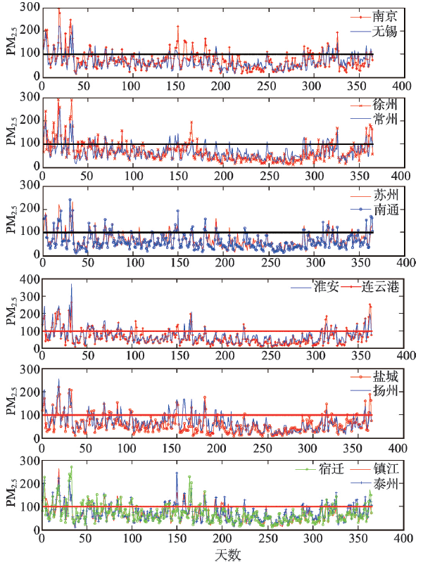
克里金空间插值法是在有限区域内对变量进行无偏最优估计的一种方法^[34],运用ArcGIS 10.0软件,对江苏省PM_2.5浓度进行空间克里金插值。插值结果检验：误差平均值为-0.1007,接近于0;标准均方根误差为0.8614,接近于1;平均标准误差为0.5454,均方根误差值为0.4699。结果表明江苏省PM_2.5浓度的空间插值结果精度高,效果好。插值结果（图1）表明,江苏省连云港、盐城、南通市3个沿海城市的PM_2.5浓度值最低,浓度最高的是南京市与泰州市。同时,江苏省PM_2.5浓度还具有南部比北部高、内陆比沿海高的趋势分布特征。通过对江苏省13个省辖市在2014年PM_2.5浓度的逐日变化（图2）分析可知,各城市PM_2.5污染较严重,浓度值超过100 μg/m³天数较多。PM_2.5浓度在11月、12月、1月,以及5月、6月出现浓度峰值;在8月、9月、10月则出现浓度谷值,同时还呈现出1月、2月PM_2.5浓度比11月、12月浓度高的趋势特征。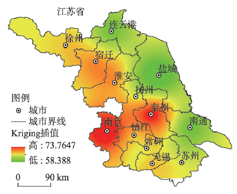

显示原图|下载原图ZIP|生成PPT
图12014年江苏省PM_2.5浓度空间变化
-->Fig. 1Spatial distribution of the PM_2.5 concentration in Jiangsu province in 2014
-->

显示原图|下载原图ZIP|生成PPT
图2江苏省13个省辖市PM_2.5浓度的逐日变化曲线
-->Fig. 2The daily change of PM_2.5 of 13 provincial cities in Jiangsu province
-->

4 结果与分析

4.1 PM_2.5浓度与影响指标关联度分析

4.1.1 指标权重系数计算与分析对原始数据进行无量纲化处理得到标准化数据,然后运用熵值赋权法,利用公式（2）、（3）、（4）计算得到影响PM_2.5浓度的指标层和指标因子的权重（w_i）（表3）。对权重值分析可知,PM_2.5污染来源指标层对江苏省PM_2.5浓度影响最大（w_i = 0.4691）,其次是空气质量指标与气象要素层（w_i = 0.2866）,城市化与产业结构层的影响最弱（w_i = 0.2453）。其中,空气质量指标与气象要素层中平均风速权重值最大,其次是NO₂、平均降雨量和平均气温;污染源指标层中,机动车保有量权重值最大,其次是公路客运量、工业用电量、氮氧化物排放量和房屋建筑施工面积;城市化与产业结构层中城市建成区面积、人口密度和地区工业总产值的权重值较大。
4.1.2 关联系数和关联度计算与分析灰色关联度（R_ij）值越大表示影响因素对PM_2.5浓度影响作用越强,贡献作用越显著,反之亦然。因此,依据关联度值可对影响PM_2.5浓度变化的指标层及指标因子按强弱进行排序。首先,计算PM_2.5浓度与指标因子间的关联度,然后计算PM_2.5浓度与指标层间的综合关联度。将影响指标因子与PM_2.5浓度标准化数据代入公式（5）,得到关联系数（表4）,对各地市关联系数之和求平均值,得到27个指标因子分别与PM_2.5浓度间的关联度值（表5）。将关联系数值代入公式（6）,得到各指标层与PM_2.5浓度的综合关联度值（表6）。
Tab. 3
表3
表3江苏省PM_2.5浓度影响评价指标体系的权重
Tab. 3Weight of the evaluation indexes system for the PM_2.5 in Jiangsu province

空气质量指标与气象要素		PM_2.5污染物来源		城市化与产业结构
w_i= 0.2866		w_i= 0.4691		w_i= 0.2453
指标因子	权重(w_i)	指标因子	权重(w_i)	指标因子	权重(w_i)
X₁	0.0889	X₁₁	0.0879	X₂₀	0.0392
X₂	0.0935	X₁₂	0.1190	X₂₁	0.1026
X₃	0.0921	X₁₃	0.0727	X₂₂	0.0924
X₄	0.1124	X₁₄	0.1622	X₂₃	0.2566
X₅	0.0752	X₁₅	0.1225	X₂₄	0.1769
X₆	0.1175	X₁₆	0.0996	X₂₅	0.0534
X₇	0.1269	X₁₇	0.1095	X₂₆	0.1051
X₈	0.1119	X₁₈	0.0970	X₂₇	0.1738
X₉	0.0930	X₁₉	0.1296	–	–
X₁₀	0.0887	–	–	–	–

新窗口打开
Tab. 4
表4
表4江苏省13个省辖市PM_2.5浓度与影响指标间的灰色关联系数矩阵
Tab. 4Grey correlation coefficient matrix of PM_2.5 of 13 provincial cities in Jiangsu province

指标体系		南京市	无锡市	徐州市	常州市	苏州市	南通市	连云港市	淮安市	盐城市	扬州市	镇江市	泰州市	宿迁市
指标层		南京市	无锡市	徐州市	常州市	苏州市	南通市	连云港市	淮安市	盐城市	扬州市	镇江市	泰州市	指标因子
空气质量指标与气象要素	X₁	1.0000	0.8093	0.6380	0.8118	0.5046	0.8474	0.5368	0.6137	0.8674	0.7413	0.9793	0.6384	0.8828
	X₂	0.3774	0.8095	0.5429	0.6108	0.5763	0.7643	0.4322	0.6804	1.0000	0.6773	0.6053	0.5127	0.6448
	X₃	0.4288	0.7470	0.5428	0.7107	0.8259	0.7074	0.4202	0.9593	0.9133	0.6184	0.5989	0.6503	0.6473
	X₄	0.9368	0.7547	0.8549	0.6917	0.4955	0.6599	0.7124	0.4344	0.8497	0.7477	0.7160	0.3588	0.6093
	X₅	0.4312	0.6257	0.9539	0.6481	0.9049	0.9586	0.7937	0.4284	0.6299	0.7162	0.9587	0.8246	0.7918
	X₆	0.5130	0.4639	0.5429	0.7006	0.6376	0.8272	0.4096	0.8935	0.9370	0.9917	0.5729	0.8318	0.8769
	X₇	0.6773	0.7537	0.4636	0.7061	0.7285	0.3866	0.9756	0.6192	0.5076	0.5791	0.5747	0.5410	0.4247
	X₈	0.6541	0.6167	0.7200	0.8161	0.4955	0.6279	0.6876	0.4621	0.8484	0.7549	0.7958	0.5006	0.4781
	X₉	0.4469	0.6891	0.4634	0.4876	0.7983	0.5945	0.6950	0.8026	0.4522	0.7323	0.5425	0.5074	0.5939
	X₁₀	0.4559	0.5499	0.5429	0.6577	0.5046	0.7919	0.6204	0.4983	0.3438	0.6876	0.6239	0.8461	0.8536
PM_2.5污染来源	X₁₁	1.0000	0.5378	0.6029	0.6745	0.7463	0.9207	0.6876	0.6105	0.7790	0.7008	0.4669	0.4114	0.4999
	X₁₂	0.4557	0.5051	0.7284	0.5671	0.4955	0.9551	0.7699	0.4843	0.8107	0.6361	0.4808	0.3839	0.4247
	X₁₃	1.0000	0.7283	0.8507	0.8613	0.8819	0.7267	0.9971	0.4886	0.7901	0.9270	0.6205	0.3682	0.4247
	X₁₄	1.0000	0.7749	0.5590	0.7736	0.6272	0.9400	0.6876	0.4500	0.9585	0.5812	0.4775	0.3709	0.4314
	X₁₅	0.5995	0.7719	0.6773	0.9214	0.4955	0.9534	0.6959	0.4679	1.0000	0.5694	0.5397	0.3784	0.4501
	X₁₆	0.5597	0.7330	0.7129	0.5085	0.4955	0.9053	0.8600	0.4833	0.7980	0.5866	0.6169	0.4073	0.4247
	X₁₇	0.5011	0.9063	0.6819	0.6551	0.4955	0.9111	0.7261	0.4937	0.8841	0.6374	0.5755	0.3795	0.4247
	X₁₈	0.9493	0.9559	0.7221	0.7488	0.4955	0.7779	0.7917	0.4724	0.6395	0.5118	0.5213	0.3588	0.6598
	X₁₉	0.4100	0.4855	0.5162	0.5576	0.6115	0.3866	0.7166	0.4762	0.7886	0.7224	0.4636	0.4679	0.4459
城市化与产业结构	X₂₀	0.3333	0.6726	0.6414	0.5446	0.6295	0.4005	0.4648	0.6237	0.3346	0.5155	0.5711	0.8246	0.6530
	X₂₁	0.4450	0.7011	0.5540	0.8915	0.7427	0.7092	0.7061	0.8301	0.4229	0.5358	0.4636	0.8246	0.8163
	X₂₂	0.3333	0.6507	0.6303	0.6742	0.9715	0.6706	0.3928	0.7782	0.3621	0.6430	0.7422	0.9319	0.7132
	X₂₃	1.0000	0.7288	0.6250	0.5859	0.8579	0.9013	0.8202	0.4694	0.9382	0.5540	0.5023	0.3674	0.4247
	X₂₄	0.4384	0.5422	0.5851	0.6982	0.7762	0.5903	0.7049	0.4652	0.8233	0.6546	0.6293	0.4251	0.4247
	X₂₅	0.3333	0.8318	0.6750	0.8051	0.7567	0.4829	0.6161	0.6489	0.3462	0.6503	0.9876	0.8249	0.8100
	X₂₆	0.6323	0.5838	0.9134	0.7155	0.4955	0.6230	0.8944	0.4633	0.6934	0.8047	0.7125	0.5489	0.4247
	X₂₇	1.0000	0.7586	0.6880	0.8828	0.5391	0.9320	0.7188	0.4968	0.8292	0.8194	0.5391	0.4279	0.4247

新窗口打开
通常,当0<R ≤ 0.30,关联度为轻度;当0.30<R ≤0.60,关联度为中度;当0.60<R ≤ 1.0,关联度为强度。对各指标因子与PM_2.5浓度的关联度值（表5）分析可知,影响指标因子与PM_2.5浓度的关联度值均较大,其关联度为中度或强度,充分显示各指标因子对PM_2.5浓度变化具有重要影响,也表明各指标因子选择较为合理。关联度为中度的指标仅包括公路客运量、房屋建筑施工面积、园林绿地面积和人口密度,PM_2.5与其余指标因子均呈强度相关联,其中与PM₁₀、O₃、降雨量、公路货运总量、地区工业总产值和第二产业占地区生产总值比重等指标的关联度相对较高。空气污染物质与气候要素是PM_2.5中的水溶性离子、多环芳烃有机物和二次污染物转化形成的重要条件。降雨量对空气中PM_2.5中尘粒具有冲洗作用,风速对降低PM_2.5浓度具有显著作用,PM_2.5属于PM₁₀中粒径更小的组成部分,公路货运汽车尾气排放是交通运输尘粒排放的主要来源,工业用电量及地区工业总产值代表了工业生产的规模与总量,工业废气烟尘排放量是空气中PM_2.5污染来源的主要组成,而园林绿地面积则对降低PM_2.5浓度具有显著作用。因此,各指标因子与PM_2.5浓度的灰色关联度较强,充分说明各指标因子对PM_2.5浓度变化具有较显著影响。
Tab. 5
表5
表5江苏省PM_2.5浓度与影响指标因子间的关联度
Tab. 5Grey correlation degree between PM_2.5 and the index of influencing factors in Jiangsu province

指标因子	X₁	X₂	X₃	X₄	X₅	X₆	X₇	X₈	X₉
关联度(R)	0.7593	0.6334	0.6746	0.6786	0.7435	0.7076	0.6106	0.6506	0.6004
指标因子	X₁₀	X₁₁	X₁₂	X₁₃	X₁₄	X₁₅	X₁₆	X₁₇	X₁₈
关联度(R)	0.6136	0.6645	0.5921	0.7435	0.6640	0.6554	0.6224	0.6363	0.6619
指标因子	X₁₉	X₂₀	X₂₁	X₂₂	X₂₃	X₂₄	X₂₅	X₂₆	X₂₇
关联度(R)	0.5422	0.5546	0.6649	0.6534	0.6750	0.5967	0.6745	0.6543	0.6967

新窗口打开
Tab. 6
表6
表6江苏省13个省辖市PM_2.5浓度与影响指标层的综合关联度
Tab. 6Synthetic grey correlation degrees between PM_2.5 and the index layers of 13 provincial cities in Jiangsu province

指标	南京市	无锡市	徐州市	常州市	苏州市	南通市	连云港市	淮安市	盐城市	扬州市	镇江市	泰州市	宿迁市
PM_2.5浓度	73.8167	67.2667	67.2833	66.4833	65.9167	61.5083	61.825	68.65	58.3	65.9333	67.275	72.1667	68.8083
R_{空气质量指标与气象要素}	0.6219	0.6918	0.6244	0.7014	0.6590	0.6993	0.5764	0.6497	0.7390	0.7204	0.6680	0.6285	0.6889
R_{污染物来源}	0.8902	0.7420	0.6613	0.7208	0.5802	0.8317	0.3476	0.5063	0.8409	0.6582	0.5415	0.8490	0.4790
R_{城市化与产业结构}	0.6511	0.6980	0.6815	0.7052	0.7270	0.7358	0.4476	0.5695	0.7118	0.6690	0.6107	0.6865	0.5431

新窗口打开
对各指标层与PM_2.5浓度的综合关联度（表6）分析可知,3个指标层中,PM_2.5污染源指标层与PM_2.5浓度关联度值较大的城市分别是南京、无锡、常州、南通、泰州市;城市化与产业结构指标层与PM_2.5浓度关联度值较大的城市分别是徐州、苏州、盐城、常州市;空气质量与气象要素指标层与PM_2.5浓度关联度值较大的城市分别是盐城、扬州、常州、南通市。不同城市各指标层与PM_2.5浓度综合关联度值差异,也充分体现出不同城市间在区域环境、社会经济、人口密度、城市产业结构、城市规模等方面对PM_2.5浓度影响的差异。

4.2 指标因子关联度与PM_2.5浓度空间分布的相关性

与PM_2.5浓度呈强度关联的23个指标在不同城市存在空间分异,表明不同城市对PM_2.5浓度的影响作用存在显著差异。影响南京市PM_2.5浓度的指标中PM₁₀、NO₂、等级公路里程、公路货运总量、机动车保有量、烟尘排放量、建成区面积、工业总产值的关联度值在所有城市中最大。苏州市影响PM_2.5浓度的指标中CO、O₃、公路货运总量、人均绿地面积等指标的关联度值较大。而临海的盐城市影响PM_2.5浓度较强指标是SO₂、CO、降雨量、平均气温和工业用电量等指标。因此,通过指标因素关联度分析,可清晰了解不同城市PM_2.5浓度变化的主要影响指标因素。
另外,综合关联度也与PM_2.5浓度空间变化有较好的关联性。连云港市、盐城市和南通市的PM_2.5浓度值在全省最低,但仅连云港市PM_2.5浓度与各指标层的综合关联度均为中度,盐城市、南通市的污染源影响指标层均与PM_2.5浓度的综合关联度为强度。分析可知,虽然盐城与南通市都有形成严重PM_2.5的污染源及污染条件,但他们的PM_2.5浓度值都较低,这是因为它们还受到临近海洋环境的削弱影响作用。南京、泰州是江苏省PM_2.5浓度值最高的城市,其PM_2.5污染来源指标层与PM_2.5浓度的综合关联度值也较高。南京PM_2.5浓度值高的最主要影响指标因素是工业生产废气排放、交通尾气与建筑施工扬尘等,这也与其实际情况吻合。无锡市、徐州市、镇江市、常州市、淮安市和苏州市的PM_2.5浓度值相差较小,但对其影响的各指标层次综合关联度值却存在明显差异,体现出不同城市PM_2.5浓度变化的影响指标层的空间分异。研究结果表明,灰色关联度模型分析法可有效分析出主要影响指标因子与PM_2.5浓度空间分布的相互关系。

5 结论

PM_2.5污染问题是目前人类社会发展中面临的非常严重环境问题,它对人类的身体健康、生态环境系统、社会生产均产生严重影响。通过构建PM_2.5浓度的影响指标体系,运用灰色关联数学分析方法对其关联度进行分析与研究,并探讨其与PM_2.5浓度空间分布的关系。结果表明：PM_2.5污染来源指标层的权重值最大,其次是空气质量与气象要素指标层,城市化与产业结构层的权重值最小;对影响指标的关联度分析表明,与PM_2.5浓度关联度为强度的是PM₁₀、O₃、CO、NO₂、SO₂、平均风速、降雨量、平均气温、平均相对湿度、照时数、等级公路里程、公路货运量、机动车保有量、工业用电量、SO₂排放量、烟（粉）尘排放量、建成区绿地覆盖率、人均公园绿地面积、建成区面积、第二产业占地区生产总值比重、人均地区生产总产值和地区工业总产值;与PM_2.5浓度关联度为中度的指标因子分别是公路客运量、房屋建筑施工面积、园林绿地面积和人口密度等4个指标因子。PM_2.5污染源指标层与PM_2.5浓度关联度值较大的城市分别是南京、无锡、常州、南通、泰州市;城市化与产业结构指标层与PM_2.5浓度关联度值较大的城市分别是徐州、苏州、盐城、常州市;空气质量与气象要素指标层与PM_2.5浓度关联度值较大的城市分别是盐城、扬州、常州、南通市。通过关联系数与关联度值分析均表明,影响指标因子关联度值与PM_2.5浓度空间分布有较好相关性。研究结果表明,灰色关联模型可有效对PM_2.5浓度主要影响因素进行定量分析与评价。
该研究中还存在一些需要改进和深入的地方：PM_2.5浓度影响指标体系仍需要改进,如增加城市交通地、居民用地等指标,考虑距海远近因素、农业生产扬尘与生物资燃烧等因素;深入研究PM_2.5浓度与影响因素间灰色关联度的时空分异及预测模型,继而探讨PM_2.5的污染与防治措施等。
The authors have declared that no competing interests exist.

参考文献原文顺序
文献年度倒序
文中引用次数倒序
被引期刊影响因子

[1]	Gehrig R, Buchmann B.Characterising seasonal variations and spatial distribution of ambient PM₁₀ and PM_2.5 concentrations based on long-term Swiss monitoring data. Atmospheric Environment, 2003, 37(19): 2571-2580.https://doi.org/10.1016/S1352-2310(03)00221-8 Magsci [本文引用: 1]摘要 <h2 class="secHeading" id="section_abstract">Abstract</h2><p id="">Collocated parallel measurements of PM2.5 and PM10 were conducted at 7 sites in Switzerland since January 1998, constituting now one of the longest comparative data sets for PM2.5 and PM10 in Europe. The range of the long-term mean concentrations of PM2.5 was between 7.9 μg/m<sup>3</sup> at Chaumont and 24.4 μg/m<sup>3</sup> in Lugano. For the sites within the Swiss plateau this range narrows from 15.1 μg/m<sup>3</sup> at the rural site of Payerne to 20.8 μg/m<sup>3</sup> at the directly traffic exposed site of Bern. The long-term averages of the PM2.5/PM10 ratios of the daily values vary only from 0.75 to 0.76, with the exception of the traffic exposed site of Bern (0.59). The correlation between the daily values of PM2.5 and PM10 at all sites is generally high. For PM10, as well as for PM2.5 the highest concentrations are normally observed during wintertime. An exception is Chaumont (1140-m a.s.l.), which is often positioned above the inversion layer during wintertime and, therefore, has the lowest concentration during wintertime. A minimum of the PM2.5/PM10 ratio is often found during spring, probably due to the influence of relatively coarse biogenic particles. Though the sites have quite different exposition characteristics, the correlation of the daily values of PM2.5 and PM10 between the different sites of the Swiss plateau is very high, indicating a dominant influence of regional meteorology over local events and sources. The findings imply that from the point of view of an efficient use of financial and personal resources, the number of collocated PM2.5 measurements at PM10 sites in a monitoring network can be kept quite limited. The saved resources could rather be used to investigate other particle related parameters providing substantial new information (e.g. on particle sources, formation and effects) like PM1, particle number concentrations, morphology or chemical composition.</p>
[2]	Song Yu, Tang Xiaoyan, Zhang Yuanhang, et al.Effects on fine particles by the continued high temperature weather in Beijing. Environmental Science, 2002, 23(4): 33-37.https://doi.org/10.3321/j.issn:0250-3301.2002.04.007 URL [本文引用: 1]摘要在 1 999 0 6 2 3北京市出现长达 1 3d的持续高温期间对细粒子 (PM2 5)质量浓度进行了观测 .数据表明 ,持续高温期间细粒子质量浓度比非高温期间要高出 2～ 3倍 .但是通过对持续高温期间的气象数据进行分析 ,发现还是很利于污染物扩散 .进一步分析同步监测的O3浓度、颗粒物中SO2 - 4的粒径范围及其含量等数据 ,发现夏季持续高温期间活跃的光化学反应应该是北京市细粒子的主要来源 [宋宇, 唐孝炎, 张远航, 等. 夏季持续高温天气对北京市大气细粒子(PM_2.5)的影响 . 环境科学, 2002, 23(4): 33-37.]https://doi.org/10.3321/j.issn:0250-3301.2002.04.007 URL [本文引用: 1]摘要在 1 999 0 6 2 3北京市出现长达 1 3d的持续高温期间对细粒子 (PM2 5)质量浓度进行了观测 .数据表明 ,持续高温期间细粒子质量浓度比非高温期间要高出 2～ 3倍 .但是通过对持续高温期间的气象数据进行分析 ,发现还是很利于污染物扩散 .进一步分析同步监测的O3浓度、颗粒物中SO2 - 4的粒径范围及其含量等数据 ,发现夏季持续高温期间活跃的光化学反应应该是北京市细粒子的主要来源
[3]	Wei Yuxiang, Yin Yan, Yang Weifen, et al.Analysis of the pollution characteristics influence factors of PM_2.5 in Nanjing area. Environmental Science and Management, 2009, 34(9): 29-34.https://doi.org/10.3969/j.issn.1673-1212.2009.09.008 URL摘要文章利用2007年南京市草场门和迈皋桥采样点的PM2.5在线监测资料研究了南京地区PM2.5浓度的时空变化特征。对PM2.5质量浓度进行了月季变化、日变化特征分析。并利用同时期气象资料分析了PM2.5浓度与气象条件的关系。结果表明,南京市细颗粒物污染较严重,草场门采样点各月超标率均在55%以上,年超标率达72%;2采样点各季节霾天气下PM2.5质量浓度均大于非霾日下浓度均值,不管是霾天气还是非霾天气下,草场门采样点各季节PM2.5质量浓度均高于迈皋桥采样点(除秋季非霾天气)。2007年南京市PM2.5质量浓度呈现出春冬季节较高、夏秋季节较低的特点;日变化呈双峰分布。对PM2.5质量浓度与水平能见度的相关性研究表明,南京市大气能见度与细粒子质量浓度呈现很好的负相关性,相关系数高达0.98。草场门采样点霾天气下平均能见度水平仅5.2 km,最高能见度为13 km,最低为1.7 km。 [魏玉香, 银燕, 杨卫芬, 等. 南京地区PM_2.5污染特征及其影响因素分析 . 环境科学管理, 2009, 34(9): 29-34.]https://doi.org/10.3969/j.issn.1673-1212.2009.09.008 URL摘要文章利用2007年南京市草场门和迈皋桥采样点的PM2.5在线监测资料研究了南京地区PM2.5浓度的时空变化特征。对PM2.5质量浓度进行了月季变化、日变化特征分析。并利用同时期气象资料分析了PM2.5浓度与气象条件的关系。结果表明,南京市细颗粒物污染较严重,草场门采样点各月超标率均在55%以上,年超标率达72%;2采样点各季节霾天气下PM2.5质量浓度均大于非霾日下浓度均值,不管是霾天气还是非霾天气下,草场门采样点各季节PM2.5质量浓度均高于迈皋桥采样点(除秋季非霾天气)。2007年南京市PM2.5质量浓度呈现出春冬季节较高、夏秋季节较低的特点;日变化呈双峰分布。对PM2.5质量浓度与水平能见度的相关性研究表明,南京市大气能见度与细粒子质量浓度呈现很好的负相关性,相关系数高达0.98。草场门采样点霾天气下平均能见度水平仅5.2 km,最高能见度为13 km,最低为1.7 km。
[4]	Zhao Chenxi, Wang Yunqi, Wang Yujie, et al.Temporal and spatial distribution of PM_2.5 and PM₁₀ pollution status and the correlation of particulate matters and meteorological factors during winter and spring in Beijing. Environmental Science, 2014, 35(2): 418-427. [本文引用: 1] [赵晨曦, 王云琦, 王玉杰, 等. 北京地区冬春PM_2.5和PM₁₀污染水平时空分布及其与气象条件的关系 . 环境科学, 2014, 35(2): 418-427.] [本文引用: 1]
[5]	Wei Fusheng, Teng Enjiang, Wu Guoping, et al.Concentrations and elemental components of PM_{2. 5}、PM₁₀ in ambient air in four large Chinese cities. Environmental Monitoring in China, 2001, 17(7): 1-6.URL [本文引用: 1]摘要报告了 1 995～ 1 996年在中国的广州、武汉、兰州、重庆 4大城市 8个采样点 PM2 .5 、PM2 .5～ 1 0 和 PM1 0 的监测结果。结果表明 ,1 995年 PM2 .5 年均值浓度为 57～ 1 60 μg/m3,比美国 1 997年颁布的标准值 (1 5μg/m3)高 2 .8～ 9.7倍。PM1 0 年日均值为 95～ 2 73μg/m3。除武汉市 1个对照点外 ,其余 7个监测点的 PM1 0 均超过我国空气质量二极标准 (1 0 0μg/m3)2 8%～ 1 73 % ,比美国标准 (50μg/m3)超过更多 ,说明污染是相当严重的。用 XRF分析了 PM2 .5 、PM2 .5～ 1 0 中 4 2种化学元素 ,结果表明 ,燃煤、燃油和其它工业污染的元素 As、Pb、Se、Zn、Cu、Cl、Br、S在这些颗粒物中有明显富集 ,特别是在PM2 .5 中的富集倍数达数十倍至数万倍 ,对人体健康有很大危害 [魏复盛, 滕恩江, 吴国平, 等. 我国4个大城市空气PM_2.5、PM₁₀污染及其化学组成 . 中国环境监测, 2001, 17(7): 1-6.]URL [本文引用: 1]摘要报告了 1 995～ 1 996年在中国的广州、武汉、兰州、重庆 4大城市 8个采样点 PM2 .5 、PM2 .5～ 1 0 和 PM1 0 的监测结果。结果表明 ,1 995年 PM2 .5 年均值浓度为 57～ 1 60 μg/m3,比美国 1 997年颁布的标准值 (1 5μg/m3)高 2 .8～ 9.7倍。PM1 0 年日均值为 95～ 2 73μg/m3。除武汉市 1个对照点外 ,其余 7个监测点的 PM1 0 均超过我国空气质量二极标准 (1 0 0μg/m3)2 8%～ 1 73 % ,比美国标准 (50μg/m3)超过更多 ,说明污染是相当严重的。用 XRF分析了 PM2 .5 、PM2 .5～ 1 0 中 4 2种化学元素 ,结果表明 ,燃煤、燃油和其它工业污染的元素 As、Pb、Se、Zn、Cu、Cl、Br、S在这些颗粒物中有明显富集 ,特别是在PM2 .5 中的富集倍数达数十倍至数万倍 ,对人体健康有很大危害
[6]	Bao Zhen, Feng Yinchang, Jiao Li.Characterization and source apportionment of PM_2.5 and PM₁₀ in Hangzhou. Environmental Monitoring in China, 2010, 26(2): 44-48.URL摘要 2006年在杭州市两个环境受体点位采集不同季节大气中PM和PM样品,同时采集了多种颗粒物源类样品,分析了其质量浓度和多种化学成分,包括21种无机元素、5种无机水溶性离子以及有机碳和元素碳等,并据此构建了杭州市PM和PM的源与受体化学成分谱;用化学质量平衡(CMB)受体模型解析其来源。结果表明,杭州市PM和PM污染较严重,其年均浓度分别为77.5μg/m和111.0μg/m;各主要源类对PM的贡献率依次为机动车尾气尘21.6%、硫酸盐18.8%、煤烟尘16.7%、燃油尘10.2%、硝酸盐9.9%、土壤尘8.2%、建筑水泥尘4.0%、海盐粒子1.5%。各主要源类对PM贡献率依次为土壤尘17.0%、机动车尾气尘16.9%、硫酸盐14.3%、煤烟尘13.9%、硝酸盐粒8.2%、建筑水泥尘8.0%、燃油尘5.5%、海盐粒子3.4%、冶金尘3.2%。 [包贞, 冯银厂, 焦荔. 杭州市大气PM_2.5和PM₁₀污染特征及来源解析 . 中国环境监测, 2010, 26(2): 44-48.]URL摘要 2006年在杭州市两个环境受体点位采集不同季节大气中PM和PM样品,同时采集了多种颗粒物源类样品,分析了其质量浓度和多种化学成分,包括21种无机元素、5种无机水溶性离子以及有机碳和元素碳等,并据此构建了杭州市PM和PM的源与受体化学成分谱;用化学质量平衡(CMB)受体模型解析其来源。结果表明,杭州市PM和PM污染较严重,其年均浓度分别为77.5μg/m和111.0μg/m;各主要源类对PM的贡献率依次为机动车尾气尘21.6%、硫酸盐18.8%、煤烟尘16.7%、燃油尘10.2%、硝酸盐9.9%、土壤尘8.2%、建筑水泥尘4.0%、海盐粒子1.5%。各主要源类对PM贡献率依次为土壤尘17.0%、机动车尾气尘16.9%、硫酸盐14.3%、煤烟尘13.9%、硝酸盐粒8.2%、建筑水泥尘8.0%、燃油尘5.5%、海盐粒子3.4%、冶金尘3.2%。
[7]	Xiao Zhimei, Bi Xiaohui, Feng Yinchang, et al.Source apportionment of ambient PM₁₀ and PM_2.5 in urban area of Ningbo city. Research of Environmental Sciences, 2012, 25(5): 549-555.URL [本文引用: 1]摘要 2010年在宁波3个环境受体点采集不同季节的PM10和PM2.5样品,同时采集颗粒物源类样品,分析它们的质量浓度及多种无机元素、水溶性离子和碳等组分的含量.采用OC/EC最小比值法确定了SOC（二次有机碳）对PM10和PM2.5的贡献,据此重新构建了受体化学成分谱.使用化学质量平衡模型对宁波市区的PM10和PM2.5来源进行了解析.结果表明：城市扬尘、煤烟尘、二次硫酸盐和机动车尾气尘是环境空气中PM10的主要来源,其分担率分别为23.0%、15.9%、13.3%和12.3%;对PM2.5有重要贡献的源类是城市扬尘、煤烟尘、二次硫酸盐、机动车尾气尘、二次硝酸盐和SOC,其分担率分别为19.9%、14.4%、16.9%、15.2%、9.78%和8.85%. [肖致美, 毕晓辉, 冯银厂, 等. 宁波市环境空气中PM₁₀和PM_2.5来源解析 . 环境科学研究, 2012, 25(5): 549-555.]URL [本文引用: 1]摘要 2010年在宁波3个环境受体点采集不同季节的PM10和PM2.5样品,同时采集颗粒物源类样品,分析它们的质量浓度及多种无机元素、水溶性离子和碳等组分的含量.采用OC/EC最小比值法确定了SOC（二次有机碳）对PM10和PM2.5的贡献,据此重新构建了受体化学成分谱.使用化学质量平衡模型对宁波市区的PM10和PM2.5来源进行了解析.结果表明：城市扬尘、煤烟尘、二次硫酸盐和机动车尾气尘是环境空气中PM10的主要来源,其分担率分别为23.0%、15.9%、13.3%和12.3%;对PM2.5有重要贡献的源类是城市扬尘、煤烟尘、二次硫酸盐、机动车尾气尘、二次硝酸盐和SOC,其分担率分别为19.9%、14.4%、16.9%、15.2%、9.78%和8.85%.
[8]	Dockery D W, Pope C A, Xu X, et al.An association between air pollution and mortality in six US cities. New England Journal of Medicine, 1993, 329(24): 1753-1759.https://doi.org/10.1056/NEJM199312093292401 URLPMID:8179653 [本文引用: 1]摘要 The effects of air pollution on mortality are analyzed taking into account individual risk factors such as cigarette smoking. "Survival analysis including Cox proportional-hazards regression modeling was conducted with data from a 14-to-16-year mortality follow-up of 8111 adults in six U.S. cities. Mortality rates were most strongly associated with cigarette smoking. After adjusting for smoking and other risk factors we observed statistically significant and robust associations between air pollution and mortality." (EXCERPT)
[9]	Yin Yongwen, Cheng Jinping, Duan Yusen, et al.Correlation analysis between the PM_2.5, PM₁₀ which were taken in the hazy day and the number of outpatient about breathing sections, breathing sections of pediatrics in shanghai. Environmental Sciences, 2011, 32(7): 1894-1898.URL摘要为了探讨上海市霾期间PM2.5、PM10污染与呼吸科、儿呼吸科日均门诊人数的相关性;对上海市6所大中型医院2009-01-01～2009-12-31期间医院呼吸科、儿呼吸科日门诊人数及霾天PM2.5、 PM10的浓度数据运用广义相加泊松回归模型进行统计分析,并进行当日和滞后日的危险度评估.结果发现,在霾发生当日,PM10日均浓度每增加 50μg/m^3,呼吸科、儿呼吸科日均门诊人数分别增加3%和0.5%;PM2.5日均浓度每增加34μg/m^3,呼吸科、儿呼吸科日均门诊人数分别增加3.2%和1.9%;同时PM2.5、PM10污染对门诊人数影响的滞后累积效应大于当日效应,且在霾污染暴发第6 d时累积效应达到最大化.从而推测,上海市霾期间PM2.5、PM10污染对医院呼吸科、儿呼吸科日均门诊人数具有一定影响. [殷永文, 程金平, 段玉森, 等. 上海市霾期间 PM_2.5、PM₁₀污染与呼吸科、儿呼吸科门诊人数的相关分析 . 环境科学, 2011, 32(7): 1894-1898.]URL摘要为了探讨上海市霾期间PM2.5、PM10污染与呼吸科、儿呼吸科日均门诊人数的相关性;对上海市6所大中型医院2009-01-01～2009-12-31期间医院呼吸科、儿呼吸科日门诊人数及霾天PM2.5、 PM10的浓度数据运用广义相加泊松回归模型进行统计分析,并进行当日和滞后日的危险度评估.结果发现,在霾发生当日,PM10日均浓度每增加 50μg/m^3,呼吸科、儿呼吸科日均门诊人数分别增加3%和0.5%;PM2.5日均浓度每增加34μg/m^3,呼吸科、儿呼吸科日均门诊人数分别增加3.2%和1.9%;同时PM2.5、PM10污染对门诊人数影响的滞后累积效应大于当日效应,且在霾污染暴发第6 d时累积效应达到最大化.从而推测,上海市霾期间PM2.5、PM10污染对医院呼吸科、儿呼吸科日均门诊人数具有一定影响.
[10]	Jia Yuqiao, Zhao Xiaohong, Guo Xingbiao.Effects of PM₁₀ and PM_2.5 on secretion of inflammatory factors in human lung fibroblast cell. Journal of Environment and Health, 2011, 28(3): 206-208. [贾玉巧, 赵晓红, 郭新彪. 大气颗粒物PM₁₀和PM_2.5对人肺成纤维细胞及其炎性因子分泌的影响 . 环境与健康杂志, 2011, 28(3): 206-208.]
[11]	Wang Wengming, Sheng Huiping, Huang Yunbiao, et al.The PM_2.5 fine particulate pollution states and its impact on human health. Shanghai Journal of Preventive Medicine, 2015, 27(5): 290-295. [本文引用: 1] [王文朋, 沈惠平, 黄云彪, 等. 大气PM_2.5细颗粒物污染状况及对人体健康的影响 . 上海预防医学, 2015, 27(5): 290-295.] [本文引用: 1]
[12]	Buseck P R, POsfai M.Airborne minerals and related aerosol particles: effects on climate and the environment. Proceedings of the National Academy of Sciences, 1999, 96(7): 3372-3379.https://doi.org/10.1073/pnas.96.7.3372 URLPMID:10097046 [本文引用: 1]摘要 Aerosol particles are ubiquitous in the troposphere and exert an important influence on global climate and the environment. They affect climate through scattering, transmission, and absorption of radiation as well as by acting as nuclei for cloud formation. A significant fraction of the aerosol particle burden consists of minerals, and most of the remainder- whether natural or anthropogenic-consists of materials that can be studied by the same methods as are used for fine-grained minerals. Our emphasis is on the study and character of the individual particles. Sulfate particles are the main cooling agents among aerosols; we found that in the remote oceanic atmosphere a significant fraction is aggregated with soot, a material that can diminish the cooling effect of sulfate. Our results suggest oxidization of SO2 may have occurred on soot surfaces, implying that even in the remote marine troposphere soot provided nuclei for heterogeneous sulfate formation. Sea salt is the dominant aerosol species (by mass) above the oceans. In addition to being important light scatterers and contributors to cloud condensation nuclei, sea-salt particles also provide large surface areas for heterogeneous atmospheric reactions. Minerals comprise the dominant mass fraction of the atmospheric aerosol burden. As all geologists know, they are a highly heterogeneous mixture. However, among atmospheric scientists they are commonly treated as a fairly uniform group, and one whose interaction with radiation is widely assumed to be unpredictable. Given their abundances, large total surface areas, and reactivities, their role in influencing climate will require increased attention as climate models are refined.
[13]	Tsai Y I, Kuoc S C, Lee W J, et al.Long-term visibility trends in one highly urbanized, one highly industrialized, and two rural areas of Taiwan. Science of Total Environment, 2007, 382(2/3): 324-341.https://doi.org/10.1016/j.scitotenv.2007.04.048 URLPMID:17544482 [本文引用: 1]摘要 Visibility trends on the island of Taiwan were investigated employing visibility and meteorological (1961-2003), and air pollutant (1994-2003) data from one highly urbanized center (Taipei), one highly industrialized center (Kaohsiung), and two rural centers (Hualien and Taitung). Average annual visibility (1961-2003) was significantly higher at the rural centers. Unlike at the other centers, visibility in Taipei improved between 1992 (6.6 km) and 2003 (9.9 km), and this can be linked to the construction and expansion of a mass transit rail system in Taipei, the use of which has helped reduce emissions of traffic related air pollutants, particles, and . This has left Kaohsiung with the lowest annual visibility since 1994, despite its 1961-2003 average being superior to that of Taipei. Precipitation lowers visibility, as demonstrated by the all-centers correlation coefficient for visibility and precipitation of -0.92. Hence, frequency of precipitation is one of the factors contributing to the average annual visibility number. The poorest air quality category ('episode'), most commonly experienced in Taipei and Kaohsiung, was characterized by relatively high concentrations of PM10 and NOx at those centers, with comparatively high atmospheric pressure and comparatively low visibility and wind speed. Excepting O3, pollutant concentrations were slightly higher during weekdays, although there was no consistent, significant difference in weekday-weekend visibility. Principal component analysis demonstrated that visibility was markedly reduced in Taipei, Kaohsiung, and Hualien by increased vehicular emissions, road traffic dust, and industrial activity, but not in Taitung, where visibility was as a result superior to that at the other centers and degradation in visibility was likely a response to long-range of pollutants rather than local sources. Optimal empirical regression models indicated a negative impact on visibility for each of PM10, and , particularly so for PM10, and validity of these models for Taipei, Kaohsiung, and Hualien was confirmed by correlation coefficients of simulated and observed average visibility of 0.63-0.72 for daily visibility and 0.85-0.88 for monthly visibility. For Taitung these figures were only 0.46 and 0.50, respectively, indicating that simulations for Taitung should include long-range as a pollutant source.
[14]	Viana M, Kuhlbusch T A, Querol X, et al.Source apportionment of particulate matter in Europe: A review of methods and results. Journal of Aerosol Science, 2008, 39(10): 827-849.https://doi.org/10.1016/j.jaerosci.2008.05.007 URL Magsci [本文引用: 1]摘要 European publications dealing with source apportionment (SA) of atmospheric particulate matter (PM) between 1987 and 2007 were reviewed in the present work, with a focus on methods and results. The main goal of this meta-analysis was to provide a review of the most commonly used SA methods in Europe, their comparability and results, and to evaluate current trends and identify possible gaps of the methods and future research directions. Our analysis showed that studies throughout Europe agree on the identification of four main source types ( PM 10 PM 10 mathContainer Loading Mathjax and PM 2.5 PM 2.5 mathContainer Loading Mathjax ): a vehicular source (traced by carbon/Fe/Ba/Zn/Cu), a crustal source (Al/Si/Ca/Fe), a sea-salt source (Na/Cl/Mg), and a mixed industrial/fuel-oil combustion ( V / Ni / SO 4 2 - mathContainer Loading Mathjax ) and a secondary aerosol ( SO 4 2 - / NO 3 - / NH 4 + ) mathContainer Loading Mathjax source (the latter two probably representing the same source type). Their contributions to bulk PM levels varied widely at different monitoring sites, and showed clear spatial patterns in the cases of the crustal and sea-salt sources. Other specific sources such as biomass combustion or shipping emissions were rarely identified, even though they may contribute significantly to PM levels in specific locations.
[15]	Zhu Xianlei, Zhang Yuanhang, Zeng Limin, et al.Source identification of ambient PM_2.5 in Beijing. Research of Environmental Sciences, 2005, 18(5): 1-5.https://doi.org/10.3321/j.issn:1001-6929.2005.05.001 URL摘要 2000-2001年在北京联合大学化学学院、中国预防科学研究院和中国环境科学研究院3个采样点采集北京市PM2.5样品,并对其中无机元素、阴阳离子、有机碳(OC)、元素碳(EC)和有机物进行测定.以多环芳烃和部分无机组分为示踪物,利用CMB受体模型对PM2.5来源进行解析.结果表明,北京市PM2.5的主要来源为燃煤、扬尘、机动车排放、建筑尘、生物质燃烧、二次硫酸盐和硝酸盐及有机物.污染源贡献率随地域变化不大,燃煤、扬尘、生物质燃烧、二次硫酸盐和硝酸盐随季节变化比较明显.与1989-1990年解析结果相比,10年间PM2.5来源发生了一定变化. [朱先磊, 张远航, 曾立民, 等. 北京市大气细颗粒物PM_2.5的来源研究 . 环境科学研究, 2005, 18(5): 1-5.]https://doi.org/10.3321/j.issn:1001-6929.2005.05.001 URL摘要 2000-2001年在北京联合大学化学学院、中国预防科学研究院和中国环境科学研究院3个采样点采集北京市PM2.5样品,并对其中无机元素、阴阳离子、有机碳(OC)、元素碳(EC)和有机物进行测定.以多环芳烃和部分无机组分为示踪物,利用CMB受体模型对PM2.5来源进行解析.结果表明,北京市PM2.5的主要来源为燃煤、扬尘、机动车排放、建筑尘、生物质燃烧、二次硫酸盐和硝酸盐及有机物.污染源贡献率随地域变化不大,燃煤、扬尘、生物质燃烧、二次硫酸盐和硝酸盐随季节变化比较明显.与1989-1990年解析结果相比,10年间PM2.5来源发生了一定变化.
[16]	Cheng Hairong, Wang Zuwu, Feng Jialiang, et al.Carbonaceous species composition and source apportionment of PM_2.5 in urban atmosphere of Wuhan. Ecology and Environmental Sciences, 2012, 21(9): 1574-1579.URL [本文引用: 1]摘要大气细颗粒物(PM2.5)和碳组分(OC,EC)是影响大气能见度、气候变化以及人体健康的重要污染物,研究大气颗粒物及其中碳组分的污染特征及各类典型污染源对大气细颗粒物及碳组分的贡献,对于认识区域和城市大气污染状况,控制细颗粒物的污染,具有重要意义。2011年7月至2012年2月,利用大流量PM2.5采样器采集武汉市大气细颗粒物样品并对其碳组分进行测定。武汉市城区大气中PM2.5、OC和EC的质量浓度平均值分别为(127±48.7)、(19.4±10.5)和(2.9±1.48)μg·m-3。其PM2.5的浓度处于我国主要城市的中等偏高水平,而OC、EC的浓度则属中等偏下水平,但均高于国外城市。武汉市大气PM2.5质量浓度的季节性变化呈现出秋季冬季夏季的趋势,是气象因素和污染源排放综合影响的结果。OC浓度和EC浓度具有较好的相关性(r2=0.69),表明二者存在来源联系。OC/EC的比值为6.7,指示武汉市大气中OC和EC的来源受汽车尾气排放和生物质燃烧的共同影响。SOA的平均质量浓度值为12.5μg·m-3约占PM2.5平均质量浓度的9.8%,表明SOA对武汉市城区大气PM2.5具有重要贡献。结合PM2.5所含的水溶性离子、微量元素组成,利用正矩阵因子分析(PMF)模型对武汉市城区大气PM2.5来源进行解析,结果表明,其主要来源及贡献率分别为机动车源(27.1%)、二次硫酸盐和硝酸盐(26.8%)、工厂排放(26.4%)和生物质燃烧(19.6%)。 [成海容, 王祖武, 冯家良, 等. 武汉市城区大气PM_2.5的碳组分与源解析 . 生态环境学报, 2012, 21(9): 1574-1579.]URL [本文引用: 1]摘要大气细颗粒物(PM2.5)和碳组分(OC,EC)是影响大气能见度、气候变化以及人体健康的重要污染物,研究大气颗粒物及其中碳组分的污染特征及各类典型污染源对大气细颗粒物及碳组分的贡献,对于认识区域和城市大气污染状况,控制细颗粒物的污染,具有重要意义。2011年7月至2012年2月,利用大流量PM2.5采样器采集武汉市大气细颗粒物样品并对其碳组分进行测定。武汉市城区大气中PM2.5、OC和EC的质量浓度平均值分别为(127±48.7)、(19.4±10.5)和(2.9±1.48)μg·m-3。其PM2.5的浓度处于我国主要城市的中等偏高水平,而OC、EC的浓度则属中等偏下水平,但均高于国外城市。武汉市大气PM2.5质量浓度的季节性变化呈现出秋季冬季夏季的趋势,是气象因素和污染源排放综合影响的结果。OC浓度和EC浓度具有较好的相关性(r2=0.69),表明二者存在来源联系。OC/EC的比值为6.7,指示武汉市大气中OC和EC的来源受汽车尾气排放和生物质燃烧的共同影响。SOA的平均质量浓度值为12.5μg·m-3约占PM2.5平均质量浓度的9.8%,表明SOA对武汉市城区大气PM2.5具有重要贡献。结合PM2.5所含的水溶性离子、微量元素组成,利用正矩阵因子分析(PMF)模型对武汉市城区大气PM2.5来源进行解析,结果表明,其主要来源及贡献率分别为机动车源(27.1%)、二次硫酸盐和硝酸盐(26.8%)、工厂排放(26.4%)和生物质燃烧(19.6%)。
[17]	Zhong Wuya, Yan Wei.Analysis on urban economic development in view of PM_2.5 . Urban Insight, 2013(1): 169-174.https://doi.org/10.3969/j.issn.1674-7178.2013.01.018 URL [本文引用: 1]摘要基于PM2.5的视角,阐述了PM概念、背景及其在我国当前城市的PM2.5基本现状,并就城市发展与PM2.5关系从城市生活方式、城市生产方式与区域产业结构转型三个不同层面进行探析,认为改变城市生活方式对于缓解城市PM2.5问题作用有限,而根本出路在于区域产业结构转型、升级和生产方式转变,并且以法制形式将环境成本内生化于单一的城市经济绩效考核标准,才真正有可能解决PM2.5的环境问题. [钟无涯, 颜玮. 城市经济发展与PM_2.5关系探析 . 城市观察, 2013(1): 169-174.]https://doi.org/10.3969/j.issn.1674-7178.2013.01.018 URL [本文引用: 1]摘要基于PM2.5的视角,阐述了PM概念、背景及其在我国当前城市的PM2.5基本现状,并就城市发展与PM2.5关系从城市生活方式、城市生产方式与区域产业结构转型三个不同层面进行探析,认为改变城市生活方式对于缓解城市PM2.5问题作用有限,而根本出路在于区域产业结构转型、升级和生产方式转变,并且以法制形式将环境成本内生化于单一的城市经济绩效考核标准,才真正有可能解决PM2.5的环境问题.
[18]	Qi Yuang, Zhang Yongan.Dynamic relationship between the evolution of three industries and PM_2.5 emissions in Beijing. China Population, Resources and Environment, 2015, 25(7): 15-23.https://doi.org/10.3969/j.issn.1002-2104.2015.07.003 URL [本文引用: 1]摘要基于三次产业经济增长与PM2.5排放关系视角回答PM2.5排放源争议以及减排措施的有效性问题,文章基于2008-2014年季度数据,利用X-12-ARIMA方法分析PM2.5排放数据的季节性波动,并构建向量自回归模型,实证结果显示,PM2.5排放数据不存在稳定季节性和移动季节性特征;第二、三产业经济增长是PM2.5排放的格兰杰原因;第二产业是PM2.5排放的长期主要来源,累计效应稳定在15,短期波动对PM2.5排放产生较强促排效应,但在滞后3期出现抑排效应,表明减排措施存在滞后效应;第三产业长期为抑排效应,累计效应稳定在-3,但在滞后3期出现促排效应,表明存在PM2.5排放部门;方差分解结果显示,三次产业经济增长对PM2.5排放的贡献比例为45.2%,其中第二产业〉第三产业〉第一产业,贡献率分别为33.82%,11.04%,0.36%;其余为区域传输和生活排放,区域传输贡献为28%-36%,生活排放包括私家车、生活消耗燃煤,以及居民烹饪的油烟,比例可达到20%左右。研究结果支持了PM2.5排放源中存在31.1%的机动车和14.1%的餐饮业排放,而不存在高比例的生物质燃烧排放。据此明确了当前第二产业减排措施的有效性和滞后性,以及加强第三产业减排、顶层设计京津冀区域协同减排和控制生活排放的相应措施。 [齐园, 张永安. 北京三次产业演变与PM_2.5排放的动态关系研究 . 中国人口·资源与环境, 2015, 25(7): 15-23.]https://doi.org/10.3969/j.issn.1002-2104.2015.07.003 URL [本文引用: 1]摘要基于三次产业经济增长与PM2.5排放关系视角回答PM2.5排放源争议以及减排措施的有效性问题,文章基于2008-2014年季度数据,利用X-12-ARIMA方法分析PM2.5排放数据的季节性波动,并构建向量自回归模型,实证结果显示,PM2.5排放数据不存在稳定季节性和移动季节性特征;第二、三产业经济增长是PM2.5排放的格兰杰原因;第二产业是PM2.5排放的长期主要来源,累计效应稳定在15,短期波动对PM2.5排放产生较强促排效应,但在滞后3期出现抑排效应,表明减排措施存在滞后效应;第三产业长期为抑排效应,累计效应稳定在-3,但在滞后3期出现促排效应,表明存在PM2.5排放部门;方差分解结果显示,三次产业经济增长对PM2.5排放的贡献比例为45.2%,其中第二产业〉第三产业〉第一产业,贡献率分别为33.82%,11.04%,0.36%;其余为区域传输和生活排放,区域传输贡献为28%-36%,生活排放包括私家车、生活消耗燃煤,以及居民烹饪的油烟,比例可达到20%左右。研究结果支持了PM2.5排放源中存在31.1%的机动车和14.1%的餐饮业排放,而不存在高比例的生物质燃烧排放。据此明确了当前第二产业减排措施的有效性和滞后性,以及加强第三产业减排、顶层设计京津冀区域协同减排和控制生活排放的相应措施。
[19]	Mo Li, Yu Xinxiao, Zhao Yang, et al.Correlation analysis between urbanization and particle pollution in Beijing. Ecology and Environmental Sciences, 2014, 23(5): 806-811.https://doi.org/10.3969/j.issn.1674-5906.2014.05.012 URL [本文引用: 1]摘要城市化程度的提升带来严重的资源环境问题,尤其是空气污染问题,严重影响了人类的健康。大气中的PM2.5等颗粒物已经成为影响我国城市空气质量的主要污染物。现有研究多数是对于多年来多地区的宏观研究,缺乏对于典型地区的具体数据报道。通过分析北京市PM2.5和PM10的质量浓度与不同城市化程度地区的相关关系,探索城市化程度对PM2.5等颗粒物浓度的影响。选取北京市7处具有代表性空气质量监测点,于2013年7月至10月对PM2.5和PM10的质量浓度进行连续4个月的实时监测,结合《北京市区域统计年鉴》中的城市化指标数据,包括常住人口密度、地区生产总值和林木覆盖率,对数据进行变化趋势分析、Pearson相关分析和回归分析。研究结论表明：由于北京市不同区域城市化程度不同导致颗粒物污染状况不同,每个区域的PM2.5与PM10的质量浓度虽有差异但均显著相关,PM2.5的质量浓度约占PM10的质量浓度的 60%,PM2.5是PM10的主要组成成分。城市化程度与PM2.5等颗粒物浓度有明显的关系,PM2.5等颗粒物浓度与地区生产总值和林木覆盖率显著相关,与地区生产总值呈正相关,与林木覆盖率呈负相关;与常住人口密度呈正相关趋势但并不显著相关。其中,PM2.5的质量浓度与地区生产总值的相关系数为0.875,与林木覆盖率的相关系数为-0.838;PM10的质量浓度与地区生产总值相关系数为0.947,与林木覆盖率相关系数为-0.775。总体来看,PM2.5等颗粒物浓度随城市化程度的提高而增加,北京市区域城市化程度与颗粒物污染情况关系明显。我国在快速发展城市化的同时,应关注环境与经济相协调。调整产业结构,增加植被绿化,控制污染源将有助于减少北京市大气中颗粒物的污染程度,为我国的城市化进程提供相应的支持和保障。 [莫莉, 余新晓, 赵阳, 等. 北京市区域城市化程度与颗粒物污染的相关性分析 . 生态环境学报, 2014, 23(5): 806-811.]https://doi.org/10.3969/j.issn.1674-5906.2014.05.012 URL [本文引用: 1]摘要城市化程度的提升带来严重的资源环境问题,尤其是空气污染问题,严重影响了人类的健康。大气中的PM2.5等颗粒物已经成为影响我国城市空气质量的主要污染物。现有研究多数是对于多年来多地区的宏观研究,缺乏对于典型地区的具体数据报道。通过分析北京市PM2.5和PM10的质量浓度与不同城市化程度地区的相关关系,探索城市化程度对PM2.5等颗粒物浓度的影响。选取北京市7处具有代表性空气质量监测点,于2013年7月至10月对PM2.5和PM10的质量浓度进行连续4个月的实时监测,结合《北京市区域统计年鉴》中的城市化指标数据,包括常住人口密度、地区生产总值和林木覆盖率,对数据进行变化趋势分析、Pearson相关分析和回归分析。研究结论表明：由于北京市不同区域城市化程度不同导致颗粒物污染状况不同,每个区域的PM2.5与PM10的质量浓度虽有差异但均显著相关,PM2.5的质量浓度约占PM10的质量浓度的 60%,PM2.5是PM10的主要组成成分。城市化程度与PM2.5等颗粒物浓度有明显的关系,PM2.5等颗粒物浓度与地区生产总值和林木覆盖率显著相关,与地区生产总值呈正相关,与林木覆盖率呈负相关;与常住人口密度呈正相关趋势但并不显著相关。其中,PM2.5的质量浓度与地区生产总值的相关系数为0.875,与林木覆盖率的相关系数为-0.838;PM10的质量浓度与地区生产总值相关系数为0.947,与林木覆盖率相关系数为-0.775。总体来看,PM2.5等颗粒物浓度随城市化程度的提高而增加,北京市区域城市化程度与颗粒物污染情况关系明显。我国在快速发展城市化的同时,应关注环境与经济相协调。调整产业结构,增加植被绿化,控制污染源将有助于减少北京市大气中颗粒物的污染程度,为我国的城市化进程提供相应的支持和保障。
[20]	Pateraki S, Asimakopoulos D N, Flocas H A, et al.The role of meteorology on different sized aerosol fractions (PM₁₀, PM_2.5, PM_2.5-10). Science of the Total Environment, 2012, 419: 124-135.https://doi.org/10.1016/j.scitotenv.2011.12.064 URLPMID:22285081 [本文引用: 1]摘要 The scope of the present study is to assess the influence of meteorology on different diameter particles (PM(10), PM(2.5), PM(2.5-10)) during a 53 months long experimental campaign at an urban Mediterranean area. Except for the investigation of the wind, temperature and relative humidity role, day by day synoptic conditions were classified over the Attica peninsula in order to explore as well, the role of the synoptic scale atmospheric . The strong dependence of the aerosols character on their various sources, not only explain the different diameter particles and their differentiation with the inorganic pollutants but also highlights the need for an effective emission policy. High PM(10) and PM(2.5-10) concentrations found to be closely related to the southwesterly regime, suggesting long range from the 'polluted' south sector while the general prevalence of the secondary particles generation revealed the health hazard. PM(2.5) showed a weaker correlation than the bigger particles with both the patterns and the parameters' fluctuations. Temporal pollutants variations were clearly governed by the emissions patterns while the low wind speed was not necessarily a good indicator of high concentration levels. Finally it was found that only during the open/close anticyclonic days and the southwesterly wind regime the morning levels were continuously higher than those of the night.
[21]	Yang Y, Liu X, Qu Y, et al.Formation mechanism of continuous extreme haze episodes in the megacity Beijing, China, in January 2013. Atmospheric Research, 2015, 155: 192-203.https://doi.org/10.1016/j.atmosres.2014.11.023 URL [本文引用: 1]摘要 The primary objective of this study is to investigate the formation and evolution mechanism of the regional haze in Beijing by analyzing the process of a severe haze episode that occurredfrom1 to 31 January 2013. The mass concentration of PM 2.5 and its chemical components were simultaneously measured at the Beijing urban atmospheric environmental monitoring station. The haze was characterized by a high frequency, a long duration, a large influential region and an extremely high PM 2.5 values (>0250002μg/m 3 ). The primary factors driving the haze formation were stationary atmospheric flows (in both vertical and horizontal directions), while a temperature inversion, a lower planetary boundary layer and a higher RH accelerated the formation of the regional haze. In one incident, the temperature inversion layer occurred at a height of 13002m above ground level, which prevented the air pollutants from being dispersed vertically. The regional transport of pollutants also played an important role in the formation of the haze. Wind from the south of Beijing increased from 58% in January 2012 to 63% in January 2013. Because the area to the south of Beijing is characterized by high industrial development, the unusual wind direction favored the regional transport of pollutants and severely exacerbated the haze. SO 4 261 , NO 3 61 and NH 4 + are the three major water-soluble ions that contributed to the formation of the haze. The high variability in Cl 61 and K + indicated that large quantities of coal combustion and biomass burning occurred during the haze.
[22]	Querol X, Alastuey A, Rodriguez S, et al.Monitoring of PM₁₀ and PM_2.5 around primary particulate anthropogenic emission sources. Atmospheric Environment, 2001, 35(5): 845-858.https://doi.org/10.1016/S1352-2310(00)00387-3 Magsci [本文引用: 1]摘要 <h2 class="secHeading" id="section_abstract">Abstract</h2><p id="">Investigations on the monitoring of ambient air levels of atmospheric particulates were developed around a large source of primary anthropogenic particulate emissions: the industrial ceramic area in the province of Castelló (Eastern Spain). Although these primary particulate emissions have a coarse grain-size distribution, the atmospheric transport dominated by the breeze circulation accounts for a grain-size segregation, which results in ambient air particles occurring mainly in the 2.5–10 μm range. The chemical composition of the ceramic particulate emissions is very similar to the crustal end-member but the use of high Al, Ti and Fe as tracer elements as well as a peculiar grain-size distribution in the insoluble major phases allow us to identify the ceramic input in the bulk particulate matter. PM2.5 instead of PM10 monitoring may avoid the interference of crustal particles without a major reduction in the secondary anthropogenic load, with the exception of nitrate. However, a methodology based in PM2.5 measurement alone is not adequate for monitoring the impact of primary particulate emissions (such as ceramic emissions) on air quality, since the major ambient air particles derived from these emissions are mainly in the range of 2.5–10 μm. Consequently, in areas characterised by major secondary particulate emissions, PM2.5 monitoring should detect anthropogenic particulate pollutants without crustal particulate interference, whereas PM10 measurements should be used in areas with major primary anthropogenic particulate emissions.</p>
[23]	Zheng M, Salmon L G, Schauer J J, et al.Seasonal trends in PM_2.5 source contributions in Beijing, China. Atmospheric Environment, 2005, 39(22): 3967-3976.https://doi.org/10.1016/j.atmosenv.2005.03.036 URL Magsci [本文引用: 1]摘要 The 24-h PM2.5 samples (particles with an aerodynamic diameter of 2.5 μm or less) were taken at 6-day intervals at five urban and rural sites simultaneously in Beijing, China for 1 month in each quarter of calendar year 2000. Samples at each site were combined into a monthly composite for the organic tracer analysis by GC/MS (gas chromatography/ mass spectrometry). Compared to the data obtained from other metropolitan cities in the US, the PM2.5 mass and fine organic carbon (OC) concentrations in Beijing were much higher with an annual average of 101 and 20.9 μg m
[24]	Yangyang Xie, Bin Z, Lin Z, et al.Spatiotemporal variations of PM_2.5 and PM₁₀ concentrations between 31 Chinese cities and their relationships with SO₂, NO₂, CO and O₃. Particuology, 2015, 20: 141-149.https://doi.org/10.1016/j.partic.2015.01.003 URL [本文引用: 1]摘要 The variations of mass concentrations of PM 2.5 , PM 10 , SO 2 , NO 2 , CO, and O 3 in 31 Chinese provincial capital cities were analyzed based on data from 286 monitoring sites obtained between March 22, 2013 and March 31, 2014. By comparing the pollutant concentrations over this length of time, the characteristics of the monthly variations of mass concentrations of air pollutants were determined. We used the Pearson correlation coefficient to establish the relationship between PM 2.5 , PM 10 , and the gas pollutants. The results revealed significant differences in the concentration levels of air pollutants and in the variations between the different cities. The Pearson correlation coefficients between PMs and NO 2 and SO 2 were either high or moderate (PM 2.5 with NO 2 : r 02=020.256–0.688, mean r 02=020.498; PM 10 with NO 2 : r 02=020.169–0.713, mean r 02=020.493; PM 2.5 with SO 2 : r 02=020.232–0.693, mean r 02=020.449; PM 10 with SO 2 : r 02=020.131–0.669, mean r 02=020.403). The correlation between PMs and CO was diverse (PM 2.5 : r 02=020.156–0.721, mean r 02=020.437; PM 10 : r 02=020.06–0.67, mean r 02=020.380). The correlation between PMs and O 3 was either weak or uncorrelated (PM 2.5 : r 02=02610.35 to 0.089, mean r 02=02610.164; PM 10 : r 02=02610.279 to 0.078, mean r 02=02610.127), except in Haikou (PM 2.5 : r 02=020.500; PM 10 : r 02=020.509).
[25]	Wang Zanshan, Li Yunting, Chen Tian, et al.Spatial-temporal characteristics of PM_2.5 in Beijing in 2013. Acta Geographica Sinica, 2015, 70(1): 110-120.https://doi.org/10.11821/dlxb201501009 Magsci [本文引用: 1]摘要 <p>对2013年北京市35个自动空气质量监测子站的PM<sub>2.5</sub>数据进行分析,探讨PM<sub>2.5</sub>的时间分布特征、空间分布特征以及与前体物和大气氧化性的相关性关系。结果表明,PM<sub>2.5</sub>浓度由高到低的季节依次是冬季、春季、秋季和夏季,平均浓度分别为122.8 μg·m<sup>-3</sup>、85.1 μg·m<sup>-3</sup>、84.9 μg·m<sup>-3</sup>和79.1 μg·m<sup>-3</sup>;各类监测站中浓度由高到低的依次是交通站、城区站、郊区站和区域站,平均浓度分别为102.2 μg·m<sup>-3</sup>、91.8 μg·m<sup>-3</sup>、89.1 μg·m<sup>-3</sup>和88.7 μg·m<sup>-3</sup>。PM<sub>2.5</sub>月均浓度呈波浪型分布,在1月份、3月份、6月份和10月份各出现一个峰值。全年来看,交通站PM<sub>2.5</sub>的日变化规律呈单峰型分布,其他站点呈双峰型分布。分地区来看,年均PM<sub>2.5</sub>浓度由高到低的依次是东南部、西南部、城六区、东北部和西北部。PM<sub>2.5</sub>浓度与NO<sub>2</sub>、SO<sub>2</sub>和OX浓度均为显著正相关,表明前体物和大气氧化性对PM<sub>2.5</sub>浓度有显著影响。</p> [王占山, 李云婷, 陈添, 等. 2013年北京市PM_2.5的时空分布 . 地理学报, 2015, 70(1): 110-120.]https://doi.org/10.11821/dlxb201501009 Magsci [本文引用: 1]摘要 <p>对2013年北京市35个自动空气质量监测子站的PM<sub>2.5</sub>数据进行分析,探讨PM<sub>2.5</sub>的时间分布特征、空间分布特征以及与前体物和大气氧化性的相关性关系。结果表明,PM<sub>2.5</sub>浓度由高到低的季节依次是冬季、春季、秋季和夏季,平均浓度分别为122.8 μg·m<sup>-3</sup>、85.1 μg·m<sup>-3</sup>、84.9 μg·m<sup>-3</sup>和79.1 μg·m<sup>-3</sup>;各类监测站中浓度由高到低的依次是交通站、城区站、郊区站和区域站,平均浓度分别为102.2 μg·m<sup>-3</sup>、91.8 μg·m<sup>-3</sup>、89.1 μg·m<sup>-3</sup>和88.7 μg·m<sup>-3</sup>。PM<sub>2.5</sub>月均浓度呈波浪型分布,在1月份、3月份、6月份和10月份各出现一个峰值。全年来看,交通站PM<sub>2.5</sub>的日变化规律呈单峰型分布,其他站点呈双峰型分布。分地区来看,年均PM<sub>2.5</sub>浓度由高到低的依次是东南部、西南部、城六区、东北部和西北部。PM<sub>2.5</sub>浓度与NO<sub>2</sub>、SO<sub>2</sub>和OX浓度均为显著正相关,表明前体物和大气氧化性对PM<sub>2.5</sub>浓度有显著影响。</p>
[26]	Lin Qiaoying, Chen Yongshan.Spatial variation of PM_2.5 in cities in winter and anthropogenic influencing factors in China. Journal of Ecology and Rural Environment, 2015, 31(4): 460-465.https://doi.org/10.11934/j.issn.1673-4831.2015.04.003 URL [本文引用: 1]摘要以我国114个城市冬季(2013年12月-2014年2月)公布的PM25数据为基础,结合其他相关数据,运用空间自相关分析、克里格插值法和逐步回归分析法,研究我国冬季PM2.5浓度空间分布差异及其影响因素. 结果显示,研究期间PM2.5在空间分布上具有高值集聚、低值集聚和高值邻域的低值集聚的变化特征,全局自相关系数Moran's I为0.27.PM2.5浓度分布由北到南、从内陆到沿海具有先升高后逐渐降低的变化趋势,高浓度区域主要集中在华北平原、长江中下游平原和陕西关中平原等地区,这些区域的冬季PM2.5平均质量浓度都达到150 μg·m-3以上,最高达250 μg·m-3.多因子逐步回归分析结果表明,人为活动对我国高浓度PM25(＞150μg·m-3)分布影响显著,对低浓度PM2.5(≤75μg·m- 3)分布影响不显著.市辖区人口密度和第二产业GDP是显著影响我国高浓度PM2.5分布的主要人为影响因子.市辖区建成区面积、全市年末总人口和市辖区道路面积等是影响我国城市间PM2.5浓度分布差异的主要人为影响因子. [林巧莺, 陈永山. 我国城市冬季PM_2.5空间特征及其人为影响因子 . 生态与农村环境学报, 2015, 31(4): 460-465.]https://doi.org/10.11934/j.issn.1673-4831.2015.04.003 URL [本文引用: 1]摘要以我国114个城市冬季(2013年12月-2014年2月)公布的PM25数据为基础,结合其他相关数据,运用空间自相关分析、克里格插值法和逐步回归分析法,研究我国冬季PM2.5浓度空间分布差异及其影响因素. 结果显示,研究期间PM2.5在空间分布上具有高值集聚、低值集聚和高值邻域的低值集聚的变化特征,全局自相关系数Moran's I为0.27.PM2.5浓度分布由北到南、从内陆到沿海具有先升高后逐渐降低的变化趋势,高浓度区域主要集中在华北平原、长江中下游平原和陕西关中平原等地区,这些区域的冬季PM2.5平均质量浓度都达到150 μg·m-3以上,最高达250 μg·m-3.多因子逐步回归分析结果表明,人为活动对我国高浓度PM25(＞150μg·m-3)分布影响显著,对低浓度PM2.5(≤75μg·m- 3)分布影响不显著.市辖区人口密度和第二产业GDP是显著影响我国高浓度PM2.5分布的主要人为影响因子.市辖区建成区面积、全市年末总人口和市辖区道路面积等是影响我国城市间PM2.5浓度分布差异的主要人为影响因子.
[27]	Gelencsér A, May B, Simpson D, et al. Source apportionment of PM_2.5 organic aerosol over Europe: primary/secondary, natural/anthropogenic,fossil/biogenic origin . Journal of Geophysical Research: Atmospheres, 2007, (1984-2012), 112(D23).
[28]	Briggs D J, Collins S, Elliott P, et al.A Mapping urban air pollution using GIS: A regression-based approach. International Journal of Geographical Information Science, 1997, 11: 699-718.https://doi.org/10.1080/136588197242158 URL摘要 Abstract. As part of the EU-funded SAVIAH project, a regression-based methodology for mapping traffic-related air pollution was developed within a GIS environment. Mapping was carried out for NO2 in Amsterdam, Huddersfield and Prague. In each centre, surveys of NO2 , as a marker for traffic-related pollution, were conducted using passive diffusion tubes, exposed for four 2-week periods. A GIS was also established, containing data on monitored air pollution levels, road network, traffic volume, land cover, altitude and other, locally determined, features. Data from 80 of the monitoring sites were then used to construct a regression equation, on the basis of predictor environmental variables, and the resulting equation used to map air pollution across the study area. The accuracy of the map was then assessed by comparing predicted pollution levels with monitored levels at a range of independent reference sites. Results showed that the map produced extremely good predictions of monitored pollution levels, both for individual surveys and for the mean annual concentration, with r2 0.79-0.87 across 8-10 reference points, though the accuracy of predictions for individual survey periods was more variable. In Huddersfield and Amsterdam, further monitoring also showed that the pollution map provided reliable estimates of NO2 concentrations in the following year ( r2 0.59-0.86 for n 20).
[29]	Wu Jiansheng, Liao Xing, Peng Jian, et al.Simulation and influencing factors of spatial distribution of PM_2.5 concentrations in Chongqing. Environmental Science, 2015, 36(3): 759-767.https://doi.org/10.13227/j.hjkx.2015.03.001 URL摘要基于Arcgis平台,利用土地利用回归模型模拟重庆市 PM2.5浓度分布,获取了高分辨率结果图.从重庆市环保局网上获取了17个空气质量监测站点的PM2.5数据,利用16个监测点数据,结合土地利用数据、路网数据、DEM数据和人口数据建立土地利用回归模型,利用剩余的1个监测点数据来对回归映射结果进行检验.按照模型设置的变量生成方法,对监测点建立多种尺度的缓冲区,提取变量数据,最终生成了56个变量.按照土地利用回归模型的设置,56个自变量最终有3个变量进入PM2.5的回归方程,模型的 R2逐步增大,且最终R2为0.84,模型拟合程度非常好.回归方程中,与研究区PM2.5浓度空间分布相关性最大的因素是空气质量监测站点500 m范围内的农用地面积,然后依次是DEM和1000 m范围内一级公路总长度,它们与PM2.5的皮尔森相关系数依次是：0.695、-0.599和0.394.回归映射检验结果显示,检验点的误差率为 2.7％,误差可以接受.回归映射结果显示,PM2.5浓度以高值分布于主城区,沿一级公路分布趋势明显,与高层紧密相关,模拟结果与实际情况相符. [吴健生, 廖星, 彭建, 等. 重庆市PM_2.5浓度空间分异模拟及影响因子 . 环境科学, 2015, 36(3): 759-767.]https://doi.org/10.13227/j.hjkx.2015.03.001 URL摘要基于Arcgis平台,利用土地利用回归模型模拟重庆市 PM2.5浓度分布,获取了高分辨率结果图.从重庆市环保局网上获取了17个空气质量监测站点的PM2.5数据,利用16个监测点数据,结合土地利用数据、路网数据、DEM数据和人口数据建立土地利用回归模型,利用剩余的1个监测点数据来对回归映射结果进行检验.按照模型设置的变量生成方法,对监测点建立多种尺度的缓冲区,提取变量数据,最终生成了56个变量.按照土地利用回归模型的设置,56个自变量最终有3个变量进入PM2.5的回归方程,模型的 R2逐步增大,且最终R2为0.84,模型拟合程度非常好.回归方程中,与研究区PM2.5浓度空间分布相关性最大的因素是空气质量监测站点500 m范围内的农用地面积,然后依次是DEM和1000 m范围内一级公路总长度,它们与PM2.5的皮尔森相关系数依次是：0.695、-0.599和0.394.回归映射检验结果显示,检验点的误差率为 2.7％,误差可以接受.回归映射结果显示,PM2.5浓度以高值分布于主城区,沿一级公路分布趋势明显,与高层紧密相关,模拟结果与实际情况相符.
[30]	Chen Jingwen, Zou Bin, Wang Min, et al.Bayesian network in PM_2.5 concentration prediction considering data characteristics. Environmental Science & Technology, 2015, 38(11): 49-56.URL [本文引用: 1]摘要针对传统贝叶斯网络模型在样本数据不充分限制下预报精度低的缺陷,引入相似性度量方法,提出一种基于Jaccard相似性系数修正的贝叶斯网络PM_(2.5)日均浓度预报模型。在传统模型缺失对应输出时,改进贝叶斯网络模型可依据相似性原理,从历史资料筛选预报日相似样本,并基于筛选出的相似样本估算预报日PM_(2.5)浓度值。以2013年长沙市3个空气质量监测点监测数据为例,运用改进模型和传统模型在各站点不同季节典型月份开展了预报实验。结果表明:改进贝叶斯网络模型相对传统贝叶斯网络模型在5月、11月、2月的预报准确率均有不同程度的提高;同一月份,各站点预报效果无显著差异;不同月份预报效果差别明显,预报准确率从高到低依次是8月、5月、11月和2月。研究证实,引入样本相似性度量手段提高传统贝叶斯网络模型在空气质量预报中的精度具有可行性。 [陈璟雯, 邹滨, 王敏, 等. 顾及数据特征的贝叶斯网络 PM_2.5浓度预报研究 . 环境科学与技术, 2015, 38(11): 49-56.]URL [本文引用: 1]摘要针对传统贝叶斯网络模型在样本数据不充分限制下预报精度低的缺陷,引入相似性度量方法,提出一种基于Jaccard相似性系数修正的贝叶斯网络PM_(2.5)日均浓度预报模型。在传统模型缺失对应输出时,改进贝叶斯网络模型可依据相似性原理,从历史资料筛选预报日相似样本,并基于筛选出的相似样本估算预报日PM_(2.5)浓度值。以2013年长沙市3个空气质量监测点监测数据为例,运用改进模型和传统模型在各站点不同季节典型月份开展了预报实验。结果表明:改进贝叶斯网络模型相对传统贝叶斯网络模型在5月、11月、2月的预报准确率均有不同程度的提高;同一月份,各站点预报效果无显著差异;不同月份预报效果差别明显,预报准确率从高到低依次是8月、5月、11月和2月。研究证实,引入样本相似性度量手段提高传统贝叶斯网络模型在空气质量预报中的精度具有可行性。
[31]	Shannon C E.A mathematical theory of communication. ACM SIGMOBILE. Mobile Computing and Communications Review, 2001, 5(1): 3-55. [本文引用: 1]
[32]	Deng Julong.Control problems of grey systems. Systems & Control Letters, 1982, 1(5): 288-294.https://doi.org/10.1016/S0167-6911(82)80025-X URL [本文引用: 1]摘要 The stability and stabilization of a grey system whose state matrix is triangular is studied. The displacement operator and established transfer developed by the author are the indispensable tool for the grey system.
[33]	Liu Sifeng, Dang Yaoguo, Fang Zhigeng, et al.Grey System Theory and Its Application. 5th ed. Beijing: Science Press, 2010: 169-175. [本文引用: 1] [刘思峰, 党耀国, 方志耕, 等. 灰色系统理论及其应用. 5版. 北京: 科学出版社, 2010: 169-175.] [本文引用: 1]
[34]	Brus D J, Heuvelink G B.Optimization of sample patterns for universal kriging of environmental variables. Geoderma, 2007, 138(1): 86-95.https://doi.org/10.1016/j.geoderma.2006.10.016 URL [本文引用: 1]摘要 The quality of maps obtained by interpolation of observations of a target environmental variable at a restricted number of locations, is partly determined by the spatial pattern of the sample locations. A method is presented for optimization of the sample pattern when the environmental variable is interpolated with the help of exhaustively known covariates, which are assumed to be linearly related to the target variable. In this method the spatially averaged universal kriging variance (MUKV), which incorporates trend estimation error as well as spatial interpolation error, is minimized. The optimal pattern is obtained using simulated annealing. The method requires that the covariance function or variogram of the regression-residuals is known. The method is tested in a case study on the Mean Highest Water table in a coversand area in The Netherlands. The patterns of 25, 50 and 100 sample locations are optimized and compared with the patterns optimized with the ordinary kriging (OK) model (assuming no trend) and with the multiple linear regression (MLR) model (assuming no spatial autocorrelation of residuals). The results show that the UK-patterns are a good compromise between spreading in geographic space and feature space. The MUKV for the UK-patterns is 19% ( n =25), 7% ( n =50) and 3% ( n =100) smaller than for the OK-patterns. Compared with the MLR-patterns the reduction is 2%, 4% and 4%, respectively.

基于灰色关联模型对江苏省PM2.5浓度影响因素的分析

本站小编 Free考研考试/2021-12-29

Analysis of the driving factors of PM_2.5 in Jiangsu province based on grey correlation model

1 引言

2 研究方法与PM_2.5浓度影响指标数据

2.1 研究方法

2.2 PM_2.5浓度影响指标体系与数据来源

3 PM_2.5浓度时空变化特征

4 结果与分析

4.1 PM_2.5浓度与影响指标关联度分析

4.2 指标因子关联度与PM_2.5浓度空间分布的相关性

5 结论

参考文献原文顺序
文献年度倒序
文中引用次数倒序
被引期刊影响因子

相关话题/指标 城市 数据 质量 污染

领限时大额优惠券,享本站正版考研考试资料!

基于分层分区法的中国历史耕地数据的网格化重建

生计多样化背景下种植业非点源污染负荷演变

西安市城市景观的正负生态系统服务测算及空间格局

2011-2015年《地理学报（英文版）》引证指标分析

基于电子地图兴趣点的城市建成区边界识别方法

煤炭资源型城市产业结构演替与空间形态演变耦合——以安徽省淮南市为例

基于综合指标法的中国生态系统服务保护有效性评价研究

重庆市新型城镇化质量与生态环境承载力耦合分析

青藏高原东北缘马衔山夷平面特征指标的提取与分析

基于潜在语义信息的城市功能区识别----广州市浮动车GPS时空数据挖掘

基于灰色关联模型对江苏省PM2.5浓度影响因素的分析

本站小编 Free考研考试/2021-12-29

Analysis of the driving factors of PM2.5 in Jiangsu province based on grey correlation model

1 引言

2 研究方法与PM2.5浓度影响指标数据

2.1 研究方法

2.2 PM2.5浓度影响指标体系与数据来源

3 PM2.5浓度时空变化特征

4 结果与分析

4.1 PM2.5浓度与影响指标关联度分析

4.2 指标因子关联度与PM2.5浓度空间分布的相关性

5 结论

参考文献文献选项 原文顺序 文献年度倒序 文中引用次数倒序 被引期刊影响因子

相关话题/指标 城市 数据 质量 污染

Analysis of the driving factors of PM_2.5 in Jiangsu province based on grey correlation model

2 研究方法与PM_2.5浓度影响指标数据

2.2 PM_2.5浓度影响指标体系与数据来源

3 PM_2.5浓度时空变化特征

4.1 PM_2.5浓度与影响指标关联度分析

4.2 指标因子关联度与PM_2.5浓度空间分布的相关性

参考文献原文顺序
文献年度倒序
文中引用次数倒序
被引期刊影响因子

相关话题/指标城市数据质量污染