Guangcan CHEN¹,
Yunfei FU^1,2,3,,

Corresponding author: Yunfei FU,fyf@ustc.edu.cn

1.School of Earth and Space Sciences, University of Science and Technology of China, Hefei 230026, China
2.Hubei Key Laboratory for Heavy Rain Monitoring and Warning Research, Institute of Heavy Rain, China Meteorological Administration, Wuhan 430205, China
3.Anhui Meteorological Observatory, Hefei 230031, China
Manuscript received: 2020-10-21
Manuscript revised: 2021-05-19
Manuscript accepted: 2021-05-20
Abstract:Satellite microwave instruments have different field of views (FOVs) in different channels. A direct average technique (“direct method”) is frequently used to generate gridded datasets in the earth science community. A large FOV will measure radiance from outside the area of a designated grid cell. Thus, the direct method will lead to errors in a measurement over a grid cell because some pixels covering areas outside of the cell are involved in the averaging process. The Backus?Gilbert method (BG method) is proposed and demonstrated to minimize those uncertainties. Three sampling resolutions (6.5 km × 6.0 km, 11.5 km × 6.0 km, 13.0 km × 6.0 km) are analyzed based on the scanning characteristics of the Global Precipitation Measurement (GPM) Microwave Imager (GMI) 18.9-GHz channel. Brightness temperatures (TBs) at 0.5 km × 0.5 km resolution over eastern China are used to obtain synthetic 18.9-GHz TBs at the three sampling resolutions. The direct and BG methods are both applied to create a 25 km × 25 km gridded dataset and their related uncertainties are analyzed. Results indicate the error variances with the direct method are 3.00, 3.68 and 4.99 K² at the three sampling resolutions, respectively. By contrast, the BG method leads to a much smaller error variance than the direct method, especially over areas with a large TB gradient. Two GMI orbital measurements are applied to verify the BG method for gridding process is reliable. The BG method could be utilized for general purpose of creating a gridded dataset.
Keywords: Backus?Gilbert method,
optimization,
satellite passive microwave imager
摘要:星载微波辐射计不同的通道具有不同的视场角。地球科学社区经常使用直接平均的方法（直接方法）来产生格点化的微波数据。一个大视场角的像元会采样格点外的辐射数据。因为一些格点外的辐射数据被带入了这个格点，直接方法将引入测量误差。基于此，本文提出了Backus-Gilbert方法（BG方法）并分析了其降低格点化过程的误差的效果。首先，本文分析了GMI仪器的18.9-GHz通道的扫描特点并总结了三种像元间扫描间隔(6.5 km × 6.0 km, 11.5 km × 6.0 km, 13.0 km × 6.0 km)。其次中国东部区域内0.5 km × 0.5 km分辨率的合成亮温数据被用于生成这三种扫描间隔下的亮温图像用于模拟分析。然后本文用直接方法和BG方法将这些亮温图像格点化到25km × 25 km 的分辨率并分析了其格点化的误差。结果显示直接方法的误差方差分别为: 3.00, 3.68 和4.99 K²。而BG方法结果的误差方差有显著减小，特别是在高亮温梯度的区域。同时BG方法被应用于GMI两条轨道的实际测量数据中，验证了模拟分析结论的可靠性。因此BG方法可被广泛应用于产生格点化的微波数据。
关键词:Backus?Glibert方法,
最优化,
星载被动微波辐射计

HTML

--> --> -->

Passive microwave remote sensing is a commonly used method to obtain meteorological parameters and land surface parameters. Microwaves are electromagnetic waves with long wavelength, which can penetrate cloud, and can be detected day and night. Signals obtained by microwave instruments are utilized in the retrieval of cloud liquid/ice water, precipitation, soil moisture, vegetation index, etc. (Liu et al., 2001; Liu and Fu, 2007; Wang et al., 2009, 2014, 2019a, b), Over the last few decades, many microwave instruments have been launched—for instance, the Soil Moisture Active?Passive imager and the Micro-Wave Humidity Sounder, as well as other microwave imagers that use the conical scanning technique, such as the Special Sensor Microwave Imager/Sounder, the Global Precipitation Measurement (GPM) Microwave Imager (GMI), etc., to monitor changes in the Earth’s atmosphere, oceans, and land. Although scan modes of passive microwave instruments are different, the retrieval and algorithm principles based on multi-band information are similar.
Due to platform limitation, most instruments only have a paraboloidal antenna, and the antenna gain has an inverse association with wavelength when the size of the antenna is constant, meaning the fields of view (FOVs) of the high-frequency channels are smaller than those of the low-frequency channels (higher resolution). The different representativeness and beam-filling effect will cause error in the final products (Greenwald et al., 1997; Rapp et al., 2009). Up to now, the different spatial resolutions in different frequency channels, the beam-filling effect, and the overlapping effect of contiguous pixels are still the three main problems faced by passive microwave remote sensing. The overlapping effect can be used to obtain a high resolution for passive microwaves, especially at the lower frequencies (Fu et al., 2013), while the other problems need further study.
The latest generation GMI is more advanced than the TMI (Tropical Rainfall Measuring Mission (TRMM) Microwave Imager). However, the low-frequency channels of GMI still have poor resolution. The FOV of GMI at 10.6-GHz is about 32.1 km × 19.4 km, which is larger than the pixel sampling interval (6 km × 12 km). Usually, the smaller the sampling interval of adjacent pixels, the larger the overlapping part. Furthermore, GMI uses the conical scanning technique that causes different sampling intervals between pixels in different parts of the scan line (see Fig. 1). These different sampling intervals generate different overlapping effects.
Figure1. Horizontal distribution of the pixels observed by the low-frequency channel group of GMI. Blue points represent the pixel locations. The red dashed lines are the sub-satellite track, and the black dashed lines are the outline of swath. The difference between (a) and (b) is the projection only.


On the other hand, gridding meteorological data is very common and useful in the atmospheric sciences. For example, 3A GPROF (GPM Profiling Algorithm) produces global 0.25° × 0.25° (~25 km) gridded means using Level 2 GPROF data (Kummerow et al., 2001). Njoku et al. (2003) averaged the brightness temperatures onto 0.25° × 0.25° grid cells before retrieving the soil moisture. Deeter and Vivekanandan (2006) also averaged the 37- and 89-GHz brightness temperatures observed by ASMR-E onto 0.25° × 0.25° grid cells, in order to retrieve the liquid water path. There are many benefits to using gridded data. For instance, the size of the dataset is reduced, which will benefit data storage. Furthermore, doing so can facilitate comparisons of retrieval product from different instrument platforms.
Generally, researchers use the direct averaging technique (hereafter, “direct method”) to produce gridded datasets. The direct method averages all pixels in the grid box with equal weight, which is recognized as being both a simple and effective approach. Deeter and Vivekanandan (2006), for example, indicated that the direct method can reduce instrumental noise. At the same time, Heng and Fu (2014) studied TMI’s liquid water path errors at different grid resolutions. They found that the 0.25° gridded dataset retained local details in the instantaneous pixel data and that these data were suitable for analyzing weather activities from the meso to synoptic scale. However, there is a dense overlapping effect between pixels of microwave instruments. The direct method will count the overlapping part twice or more, but the non-overlapping parts only once. Therefore, the weights of different areas will vary. At the same time, the direct method does not consider the FOVs of pixels. The FOV of GMI at 10.6-GHz (32.1 km × 19.4 km) is larger than the size of 0.25° × 0.25° grid cells. When such pixels fall at the edge of the grid cells, half of the pixels’ FOVs sample radiance lies outside the grid cells. With this in mind, in the present paper, a gridded dataset at higher resolution is obtained on the premise of ensuring these errors are as small as possible.
Backus and Gilbert (1968) first proposed the Backus?Gilbert (BG) method in 1968. After many years of subsequent development, this method, which can reconstruct the brightness temperature of target pixels as observed by a virtual microwave imager, has since emerged as a complete theoretical system. It was first applied to data processing in the field of earth exploration. Green (1975) used the method to retrieve gravity profiles. Then, Stogryn (1978) attempted to use the BG method to match the FOVs of different channels of microwave imagers, in which a cost function was defined that balanced noise amplification and the matching effect. Since then, the BG method has been widely used in matching the FOVs of different channels of microwave imagers (Poe, 1990; Farrar and Smith, 1992; Long and Daum, 1998; Rapp et al., 2009; Wang et al., 2011; Petty and Bennartz, 2017; Chen et al., 2018; Zhou and Yang, 2020). In these studies, the antenna patterns of pixels are considered. Obviously, the closer the antenna pattern and grid cell size, the smaller the error caused by the gridding method. This paper uses this as a basis to discuss the advantages of the BG method.
This paper introduces the advantages of the BG method to the gridding process for low-frequency channels of microwave imagers and in so doing, promotes the BG method. The rest of the paper is organized as follows: section 2 introduces the GMI, antenna pattern, and BG method. Results from a simulation experiment are used in section 3 to quantitatively analyze the errors caused by the direct and BG methods. Then, some examples of applying the BG method to actual orbit data are presented in section 4. Finally, a discussion and conclusions are presented in section 5.

2

-->

2.1. GMI

GMI is a conical-scanning microwave imager that forms the main part of the GPM core platform. It has 13 channels, all of which—except 23-GHz and 183-GHz—are equipped with double polarization. The 13 channels are divided into two groups (S1 and S2, respectively). The low-frequency group (S1) has an incidence angle of 52°, and the instrument samples 221 points in one scan cycle with a scan range of about 152°. The high-frequency group (S2) parameters are the same as those of the low-frequency group, except for the incident angle, which is about 49°. The FOVs of the 10-, 18.9- and 89-GHz channels are 32.1 km (along-track direction) × 19.8 km (cross-track direction), 18.1 km× 11.7 km and 7.2 km× 6.4 km, respectively (Petty and Bennartz, 2017). Since GPROF officially tries to match all channels’ FOVs to that of the 18.9-GHz channel (Passive Microwave Algorithm Team Facility, 2017), this paper is based on the characteristics of the 18.9-GHz channel.
In order to intuitively understand the scanning characteristics of GMI, the spatial distribution of pixels observed by the low-frequency channel group (see Fig. 1) is displayed. As indicated, distances between adjacent pixels vary. The distance at the edge is larger than that at the center. There are different overlapping parts at different scan positions because of different sampling intervals between adjacent pixels. In this paper, the shortest distance between adjacent pixels with different scan numbers on the scan line is calculated (see Fig. 2). Figure 2a is a partly magnified plot of Fig. 1. Dashed lines connect adjacent pixels (blue) with the same scan numbers, while solid lines connect pixels whose distances are shortest. Figure 2a also shows that the dashed and solid lines do not coincide in the along-track direction, which means that the distance between adjacent pixels with the same scan number is not the shortest. Curves of the shortest distance along the scan line are shown in Fig. 2b. Black and red lines in Fig. 2b represent the cross- and along-track direction, respectively. The black line is close to a straight line, indicating that the distances between adjacent pixels in the cross-track direction are similar, while the red line shows a large difference in distance with scan numberr. Five regions can be clearly distinguished by the different slopes of the red line, and the demarcation points are around the scan numbers of 52, 93, 130 and 172. The shortest distance also changes, from 3.2 km at the edge region to 13.0 km at the center region. In this paper, a scan line is divided into three regions—namely, “edge”, “sub-edge” and “center” regions. The sampling intervals of these three regions are 6.5 km (along-track direction) × 6.0 km (cross-track direction), 11.5 km × 6.0 km and 13.0 km× 6.0 km, respectively. This paper is based on these three sampling intervals.
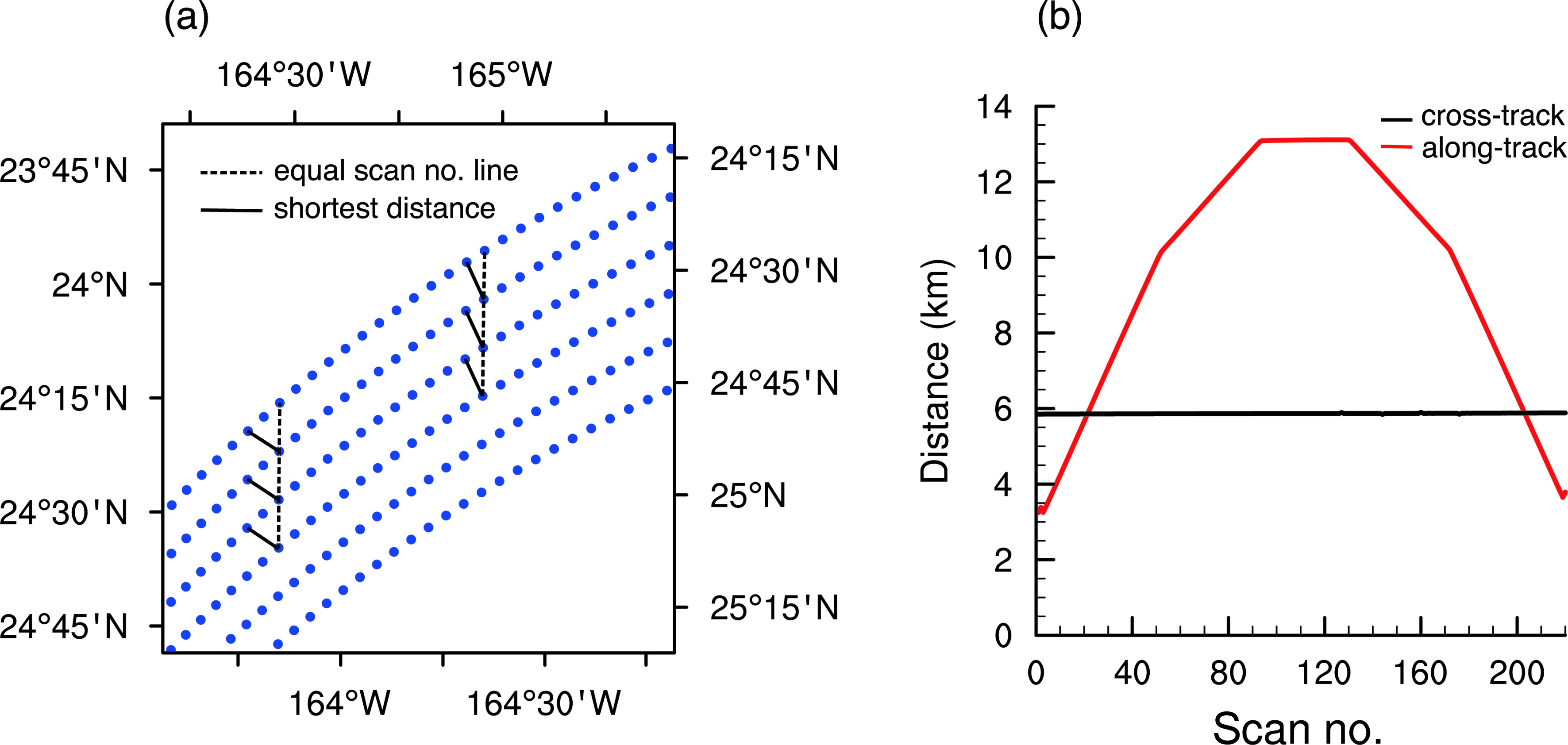Figure2. (a) Partly magnified plot of Fig. 1b, in which the pixels (blue) on the dashed line have the same scan number and the pixels on the solid line have the shortest distance. (b) Curves of shortest distance between pixels along the scan line, where the red line indicates the along-track direction and the black line the cross-track direction.



2 -->

2.2. Antenna pattern and projection

The Sinek function or Gaussian gain function is generally used to approximate antenna pattern. This paper follows previous research (Wang et al., 2011) and uses a Gaussian gain function to describe the antenna pattern:
In this application, w represents the beam width. In actual satellite observations, GMI uses the conical-scanning technique, wherein pixels at the surface approximate an ellipse, and the sizes of pixels are roughly the same. The parameters, such as beam width (w), observation location (H), azimuth ($ \varphi $), and incident angle ($ \theta $), together determine the size and shape of pixels. Because the incident angle of GMI is about 52°, all locations need to be projected from the surface coordinate system to the instrument coordinate system to calculate the antenna response. In the projection process, it is assumed that the observation axis of the instrument is the negative direction of the z-axis, and the intersection of the axis and the ground is taken as the origin to establish a new Cartesian coordinate system. The orthogonal basis ($ {\boldsymbol{A}} $) of the new coordinate system is:
Then, the coordinates of the point $ {\boldsymbol{V}}_{\rm{p}} $ on the ground in the new coordinate system can be expressed as:
In Eq. (3), z equals zero, meaning the point is on the surface. The square of the distance from $ {\boldsymbol{V}}_{\rm{p}} $ to the new z-axis is:
The projection is completed after replacing the $ x $ in Eq. (1) with $ d $ to obtain the antenna response.
Figure 3 compares two antenna patterns with beam widths of 50 km and 11.7 km before and after projection (H = 407 km, $ \varphi $ = 0°, $ \theta $ = 52°), respectively. In Fig. 3a, the curve is compressed in the direction of the satellite and stretched in the other direction. This situation is not evident in Fig. 3b. It can be seen that the projected antenna pattern gives better agreement with the actual instrument measurement than the unprojected one, especially for channels with wide beam widths. Furthermore, for the 18.9-GHz channel of GMI, projection processing seems unnecessary. In this paper, however, the 18.9-GHz antenna pattern is projected.
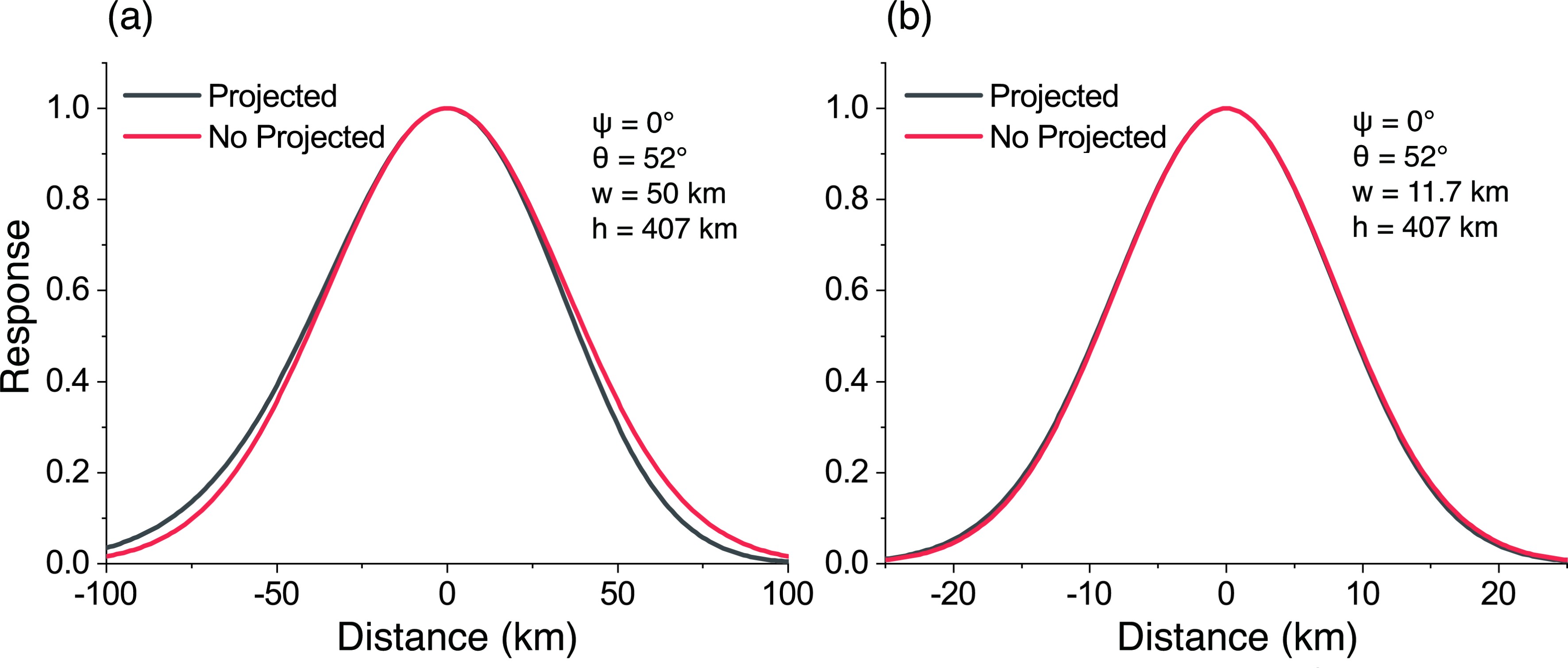Figure3. Normalized response curves of the antenna in the along-track direction before (red) and after (black) projection. The azimuth was set at 0°, the incident angle at 52°, the beam width at 50 km, and the satellite height at 407 km for (a), and the other parameters were kept the same but the beam width changed to 11.7 km for (b).



2 -->

2.3. BG method

A measured brightness temperature corresponds to a convolution of the original brightness temperature field using its antenna as a convolution kernel. The brightness temperature ($ {T}_{\rm{A}}) $ of an existing pixel can be written as
where $ {x}_{0},{y}_{0} $ represents the position of the center of the actual measured pixel. $ {T}_{\rm{B}}\left(x,y\right) $ is the original brightness temperature, and $ G $ is the sensor original antenna pattern.
The brightness temperature at a target pixel can be represented by a linear combination of the adjacent pixels’ brightness temperatures,
where $ {x}_{{\rm{d}}},{y}_{{\rm{d}}} $ represent the center position of a target pixel (virtual pixel); $ {x}_{i},{y}_{i} $ represent the center position of an actual measured pixel; $ {q}_{i} $ represents the weight coefficient, which is the solution to Eq. (15); and n is the number of adjacent pixels. In this paper, all pixels in the 50 km × 50 km gridded cells are chosen. The gridded cells have the same center as the target gridded cells (25 km × 25 km).
Eq. (5) is substituted for Eq. (6) to give:
It can be seen that the most important part of Eq. (7) is to solve all coefficients ($ {q}_{i} $). Eq. (7) is simplified to:
The function $ f $ can be viewed as an equivalent antenna pattern, and brightness temperature ($ {T}_{\rm{A}}^{'} $) would be observed by a designed imager with an equivalent antenna pattern.
Since $ f $ is the equivalent antenna pattern, it has the constraints of an antenna pattern:
The cost function ($ \varnothing) $ can be defined as
where Eq. (12) describes the theoretical brightness temperature of the target pixel. $ F $ in Eq. (11) and Eq. (12) is a designed antenna pattern of the virtual instrument. For example, in applications of mapping high-frequency channels (high-resolution) to low-frequency channels (low-resolution), $ F $ represents the low-frequency channel antenna pattern and $ G $ in Eq. (5) as the high-frequency channel antenna pattern. In this paper, the defined principle of $ F $ is to ensure that the weight at any position within the grid cell is equal and zero outside the grid, and $ G $ is the 18.9-GHz antenna pattern. $ J $ in Eq. (11) is used to deal with the sidelobe, and it has been pointed out that the effect of this part is limited, so this parameter is always set to 1 (Wang et al., 2011). To minimize the cost function, only the equivalent antenna pattern [$ f $ in Eq. (9)] can be closest to the designed target one [$ F $ in Eq. (12)].
Stogryn (1978) noted that there is noise in actual satellite observations. The noise ($ {e}^{2} $) of BG method process can be expressed as
where $ {\boldsymbol{E}} $ is the error covariance matrix, and $ {e}_{\rm{pre}}^{2} $ represent “native” instrument noise. The sum of squares of weight coefficients ($ {q}_{i} $) can be viewed as an error amplification factor. When the $ {q}_{i} $ are all positive and equal, the error amplification factor is minimized, and the BG method corresponds to the direct method. If the cost function is considered as an evaluation criterion for improving the resolution, then Eq. (13) can be considered as an evaluation criterion for the effect of error amplification while improving the resolution. Finding the balance between error amplification and resolution improvement involves dealing with a trade-off, Petty and Bennartz (2017) proposed a new cost function ($ C $):
By adjusting γ, a trade-off between resolution improvement and error amplification is considered. In this paper, an error amplification factor no greater than 1 is required. The solution to Eq. (14) is:
The matrices $ {\boldsymbol{Z}} $, $ {\boldsymbol{u}} $, and $ {\boldsymbol{v}} $ can be written as:
where $ {\delta }_{ij} $ is the Kronecker delta, $ G $ is the sensor original antenna pattern, and $ F $ is the designed antenna pattern.

In order to better understand the errors involved in the direct method, a simulation experiment was designed. Eastern China was selected as the study area in the experiment (Fig. 4a), and the range was 1000 km × 1000 km with a pixel resolution of 0.5 km × 0.5 km. The presence of ocean and lakes in the study area was consistent with actual detection. The horizontal distribution of the synthesized brightness temperature was generated by one-to-one correspondence between surface vegetation attributes and brightness temperatures in the original grid cells (Fig. 4a), and the vegetation-attribute data were obtained from the MCD12Q1 data product (available at https://lpdaac.usgs.gov/products/mcd12q1v006/). This approach, as referenced in a previous study (Limaye et al., 2006), while somewhat arbitrary, but we believe is good enough for such a simulation experiment. The raw data were gridded by the direct method to obtain the 25 km × 25 km spatial resolution (Fig. 4b), and these results are considered as the “true” values.
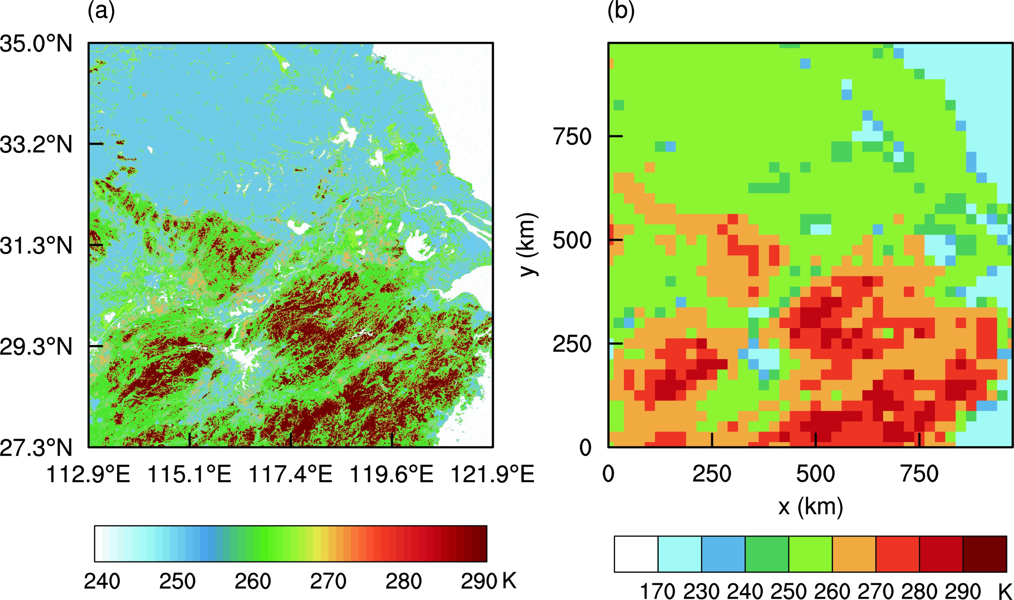Figure4. (a) Horizontal distribution of brightness temperature (0.5 km × 0.5 km) in the simulated region. (b) Horizontal distribution of gridded brightness temperature (25 km × 25 km), as processed by the direct method, from (a). The values in (b) are denoted as “true” values for the sake of clarity.


To investigate influence of the three sampling intervals on the results using the direct method, the distribution of pixels and grid lines in the simulation area was generated. The horizontal distribution of pixels (dots) and grid lines (black lines) is shown in Fig. 5 for the sampling interval of 6.5 km × 6 km (edge). Ellipses in Fig. 5 represent the FOV of 18.9-GHz pixels (18.1 km × 11.7 km). Figure 5 shows that a pixel’s measurement is a large range convolution of brightness temperatures, and overlaps exist between adjacent pixels. The figure also shows that, when a pixel is at the grid edge, its measurement will include radiance from outside the grid cell. This implies that the direct method is not appropriate for processing data that are densely overlapped and have a large FOV, where the FOV of the processed data is clearly larger than the size of a grid cell.
Figure5. Horizontal distribution of pixels and grids when the pixel interval is about 6.5 km × 6 km in the simulation experiment. Solid lines indicate the boundaries of the grid (25 km × 25 km), ellipses represent the FOVs of 18.9-GHz, points (regardless of color) represent pixel locations, and blue points indicate pixels used by the BG method.


For the three sampling intervals defined in the previous section (i.e., edge, sub-edge, and center), the horizontal distributions of pixels for 6.5 km (along-track direction) × 6 km (cross-track direction), 11.5 km × 6 km, and 13 km × 6 km were generated, respectively, using the generation approach in Fig. 5. The antenna pattern of pixels is the same as that of the GMI 18.9-GHz channel and is projected; other observation parameters are set to w = 11.7 km, H = 407 km, φ = 0°, and θ = 52°, respectively. Each pixel’s brightness temperature is calculated by convolving the brightness temperature field (0.5 km × 0.5 km) with the 18.9-GHz antenna pattern. The horizontal distributions of synthesized brightness temperatures for the three pixel sampling intervals are shown in Fig. 6. The distribution of brightness temperatures in the edge region is finer than that of the center region. The brightness temperature distribution in all three regions loses detail compared to the raw data, which is due to resolution degradation.
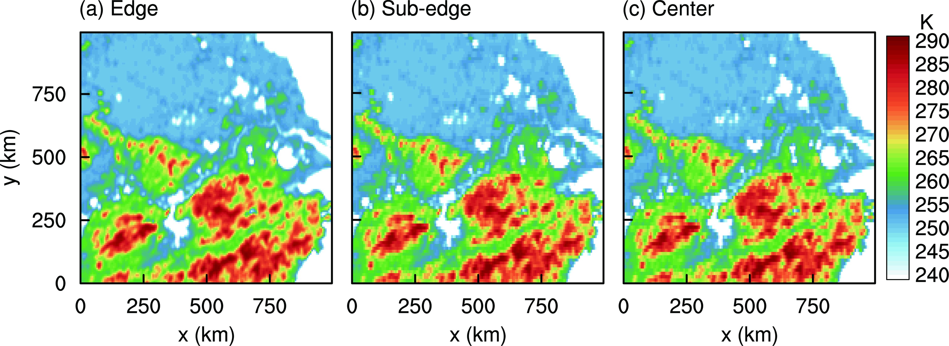Figure6. Horizontal distribution of synthesized brightness temperature for three intervals: (a) edge, 6.5 km × 6.0 km; (b) sub-edge, 11.5 km × 6.0 km; (c) center, 13.0 km × 6.0 km. The method for generating pixel locations for the three sampling intervals is shown in Fig. 5. GMI’s 18.9-GHz FOV is applied for each pixel of the three sampling intervals to obtain the synthesized brightness temperature.


The gridded results at the 25-km resolution for the three synthesized distributions in Fig. 6 are shown in Fig. 7 using the direct method. To highlight the differences and facilitate comparison, a different colorbar scale is used in Fig. 7. The three distributions in Figs. 7a-c are different from Fig. 4b, which shows the true values, but the entire distribution is the same. This shows that the direct method is a simple method when precision is not required. Results from comparing the gridded results with the true values are shown in Figs. 7d-f. The errors in Fig. 7d are smaller than those in Fig. 7f, which indicates that the results from using the direct method have smaller error for the edge region than for the center region. In addition, the figure shows that there are large errors in regions of strong gradients in brightness temperatures, such as over the coastline, indicating that the direct method will produce larger error where the gradient of the grid cell is significant. This situation is frequently found in actual observations, because the sizes of mesoscale convective systems are smaller than the FOV of the GMI’s 18.9-GHz channel. In regions such as the edge of a convective system, a strong gradient in brightness temperature is generated by the non-uniform distribution of cloud phase and height.
Figure7. (a?c) Horizontal distribution of gridded brightness temperature (25 km × 25 km), as processed by the direct method, for three intervals of pixels: (a) edge; (b) sub-edge; (c) center. (d?f) Horizontal distribution of the differences between the gridded brightness temperature and true values (see Fig. 4): (d) edge; (e) sub-edge; (f) center.


In essence, the errors of the direct method are mainly caused by the fact that the equivalent antenna pattern does not coincide with the designed antenna pattern. In other words, brightness temperature information from outside the grid cell is used in this method. The BG method is introduced to reduce this error. The advantage of the BG method is that it synthesizes an antenna pattern that is as consistent as possible with the target one by convolution and deconvolution. To compare the equivalent antenna patterns of the direct and BG methods, one grid cell in Fig. 5 (50 km?75 km in the x-direction and 25 km?50 km in the y-direction) was selected as an example. 16 pixels are used in the direct method. In this paper, all of the 72 blue pixels within the 50 km × 50 km grid cell are involved in the BG method. The center of the 50 km × 50 km grid cell coincides with the target grid cell center. So all of the 72 blue pixels have radiance contributions from this target grid cell. To strike a balance between resolution improvement and error amplification, $ \gamma $ is set to 3 × 10^?5, so the error amplification factor is less than 1.0. After determining the weights of target grid cells from Eq. (15), an equivalent antenna pattern of the grid cells can be calculated using Eq. (9).
The BG method’s equivalent antenna pattern is shown in Fig. 8b. To discuss the advantages of the BG method, the antenna patterns of the direct and BG methods in the along- and cross-track directions are compared in Figs. 8c and 8d. Black curves in Figs. 8c and 8d are extracted from Fig. 8a along the two solid lines (along- and cross-track), and have been normalized. Red and blue curves are the same as black curves but extracted from Fig. 8b and the designed antenna pattern, respectively. The direct method’s antenna patterns in Figs. 8c and 8d (black) are significantly different from the designed one (blue) in both the along- and cross-track direction. The distance between the two half-power (50% of max response) points of the BG method is closer to 25 km than that of the direct method. Therefore, the equivalent antenna pattern of the BG method (red) is reasonable.
Figure8. Equivalent antenna pattern [$ f $ in Eq. (9)] of the example grid in Fig. 5 using the (a) direct and (b) BG method. Black curves in (c, d) are extracted from (a) along the two solid lines (along- and cross-track), and it has been normalized. Red and blue curves are the same as black curves but extracted from (b) and the designed antenna pattern, respectively.


Figures 9a-c give the results of the three synthesized brightness temperatures in Fig. 6 processed by the BG method to 25-km grid cells. Figures 9d-f, meanwhile, show the errors between the gridded results and the true values. It can be seen from Figs. 9d-f that the grid cell error of the BG method is smaller. The error in Fig. 9d is also smaller than that in Fig. 9f, which indicates that the BG method’s effectiveness is limited when adjacent pixels are badly overlapped. When Petty and Bennartz (2017) matched the FOVs of GMI, they also found that the 89-GHz channels were badly overlapped in the cross-track direction, and the synthetic FOV fitted to the target effective FOV was poor in that direction.
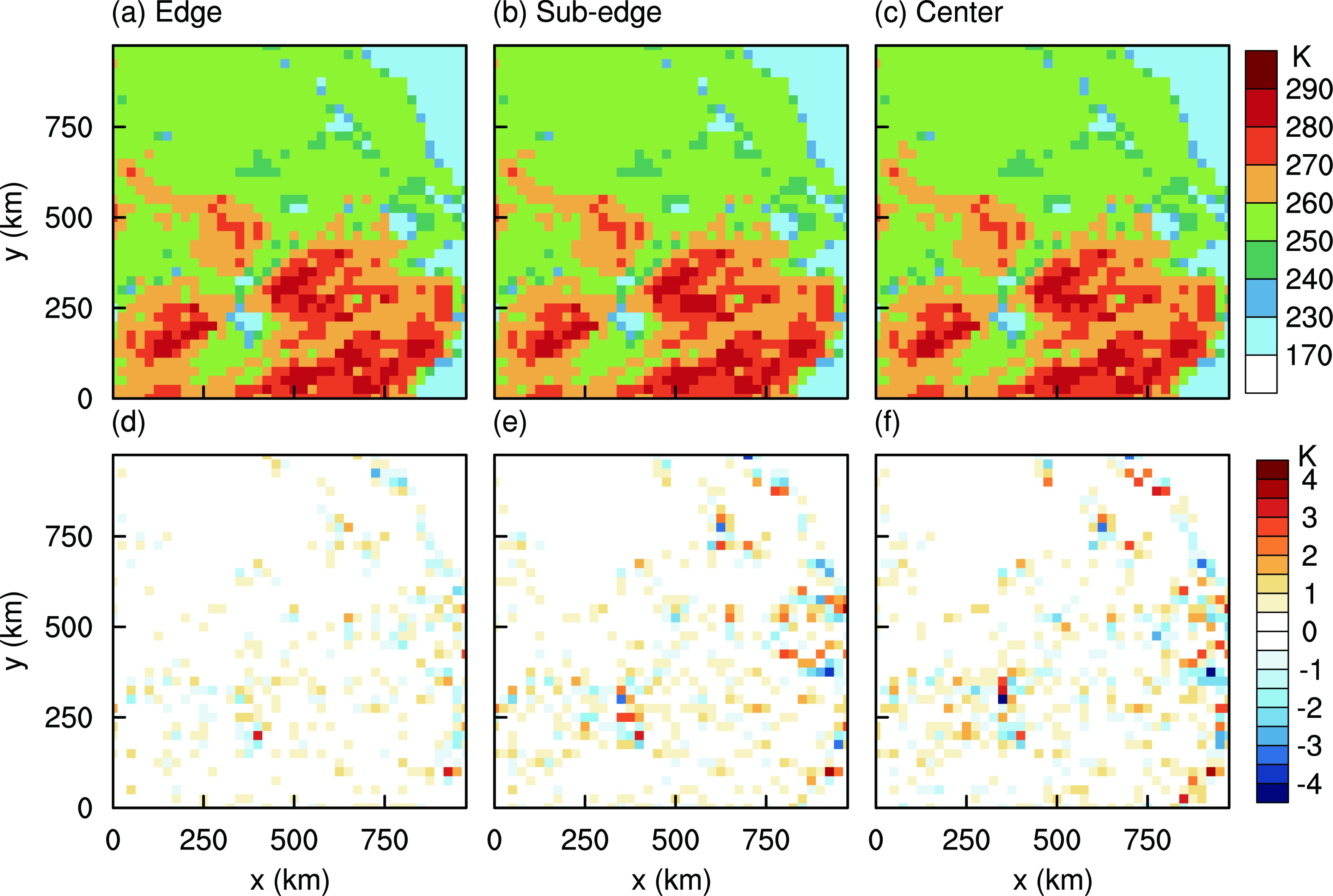Figure9. As in Fig. 7 but using the BG method.


In order to quantify these errors, the mean, error variance, and correlation coefficients for two methods’ results were calculated, separately. As Table 1 shows, the three cases’ mean values from using the direct method are almost the same as the true values, but the error variances are 3.00, 3.62 and 4.99 K², respectively. This error is greater than the inherent instrumental noise of the GMI’s 18.9-GHz channel. Combined with the information from Fig. 7, these errors are mainly associated with regions displaying strong gradients in brightness temperature. The correlation coefficients between the direct method and true values are greater than 0.99, which indicates that the direct method’s results do not change the spatial distribution of the data. The error variances of the BG method are 0.22, 0.42 and 0.49 K², respectively, which are only about 10% of those of the direct method. Because the BG method uses pixels whose center is outside the study region when computing the result of the grid edge of the study area, the average values of the BG method differ significantly from the true values. The correlation coefficients of the BG method are also higher than those of the direct method. These results show that the BG method produces smaller error and higher correlation coefficients than the direct method, which indicates that the data quality of the BG method is higher than that of the direct method.

Cases	Edge			Sub-edge			Center
	Mean (K)	Variance / R2 (K2)		Mean (K)	Variance / R2 (K2)		Mean (K)	Variance / R2 (K2)
True values	251.59	?		251.59	?		251.59	?
Direct method	251.68	3.00/0.9976		251.60	3.68/0.9971		251.63	4.99/0.9959
BG method	251.68	0.22/0.9998		251.71	0.42/0.9997		251.70	0.49/0.9996

Table1. Mean, variance of error, and correlation coefficient of the direct method and BG method.


In order to examine the consistency and reliability of the results, the simulation experiment was repeated at another location, and the results were consistent and reliable. For brevity, the related figures can be found in the electronic supplementary material (ESM, Figs. S1?S3, Table S1).

The BG method, which can greatly reduce the error of gridded results, was applied to two actual orbits. The orbit numbers of these orbits are 14 216 (example 1) and 11 386 (example 2), respectively. The 18.9-GHz vertically (V) polarized channel brightness temperatures are shown in Figs. 10a (example 1) and 10d (example 2). The direct method’s gridded results are shown in Figs. 10b and 10e, while Figs. 10c and 10f show the gridded results of the BG method. Orbit 11 386 passes over the ocean, while orbit 14 216 passes over the Tibetan Plateau. Figures 10a and b show that there are some small-scale regions of high brightness temperature in each area. Because 18.9-GHz is near the water absorption line at 22.235-GHz, the channel is influenced by precipitating water content. The high brightness temperature regions indicate a high water content in example 2. The results from using the direct and BG methods have large differences in these regions. To investigate the relationship between the differences in the results of the two methods and the brightness temperature gradient, we calculated the horizontal gradient field for each orbit’s data (example 1: Fig. 11c; example 2: Fig. 11d), as well as the horizontal distribution of the differences between the direct and BG methods (example 1: Fig. 11a; example 2: Fig. 11b). The figures show that the errors of the two methods are larger in regions of large brightness temperature gradient, which is similar to the results from the simulation experiment. This finding demonstrates that the BG method can better preserve information in these regions, such as mesoscale convective systems and cloud boundaries, and reduce the errors of gridded data. The quality of subsequent retrieval products could then also be improved.
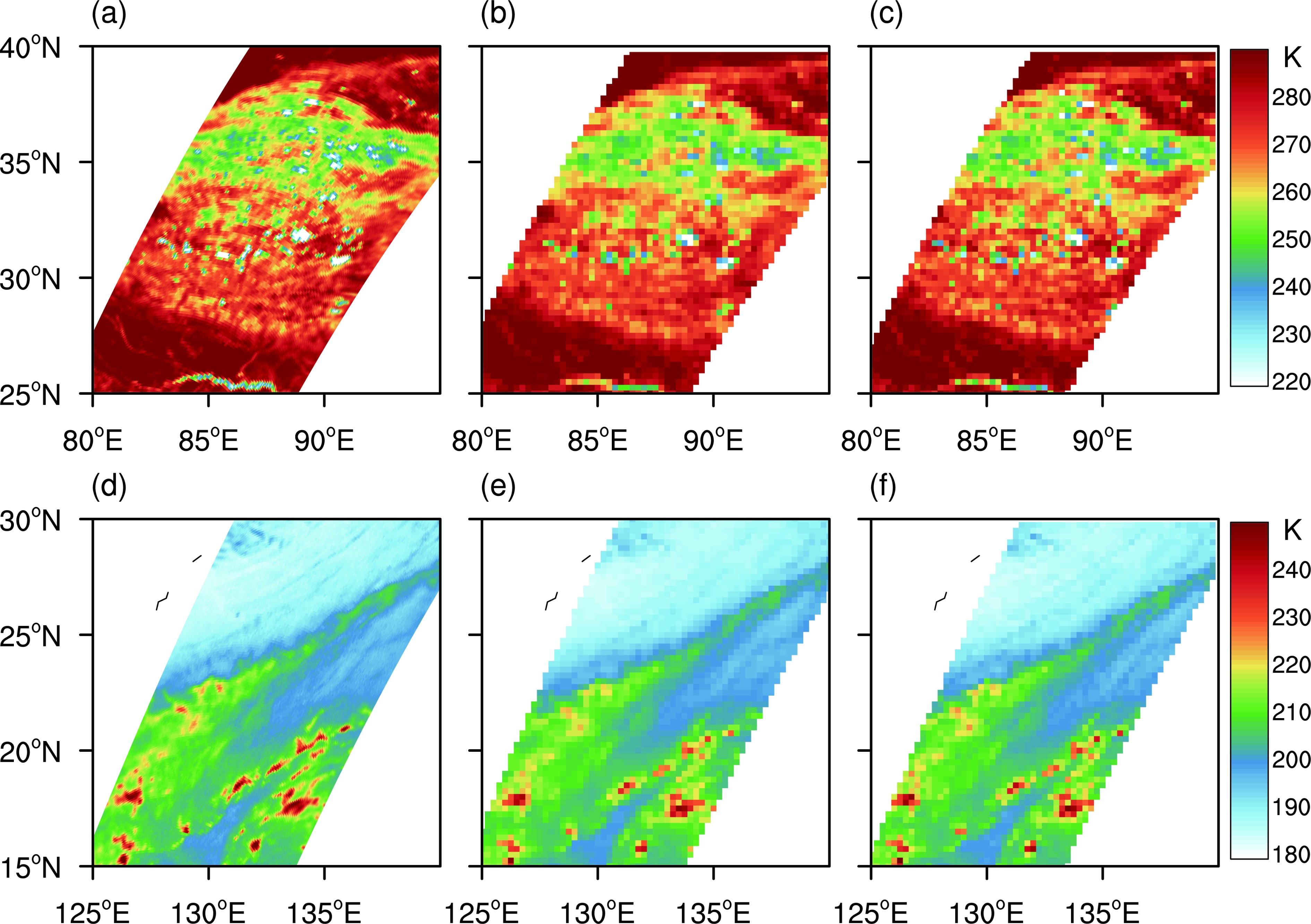Figure10. Horizontal distribution of (a) GMI 18.9-GHz V brightness temperature, and the gridded result (0.25° × 0.25°) of the (b) direct method and (c) BG method. Orbit number: 14 216. (d?f) As in (a?c) but for orbit number 11386.


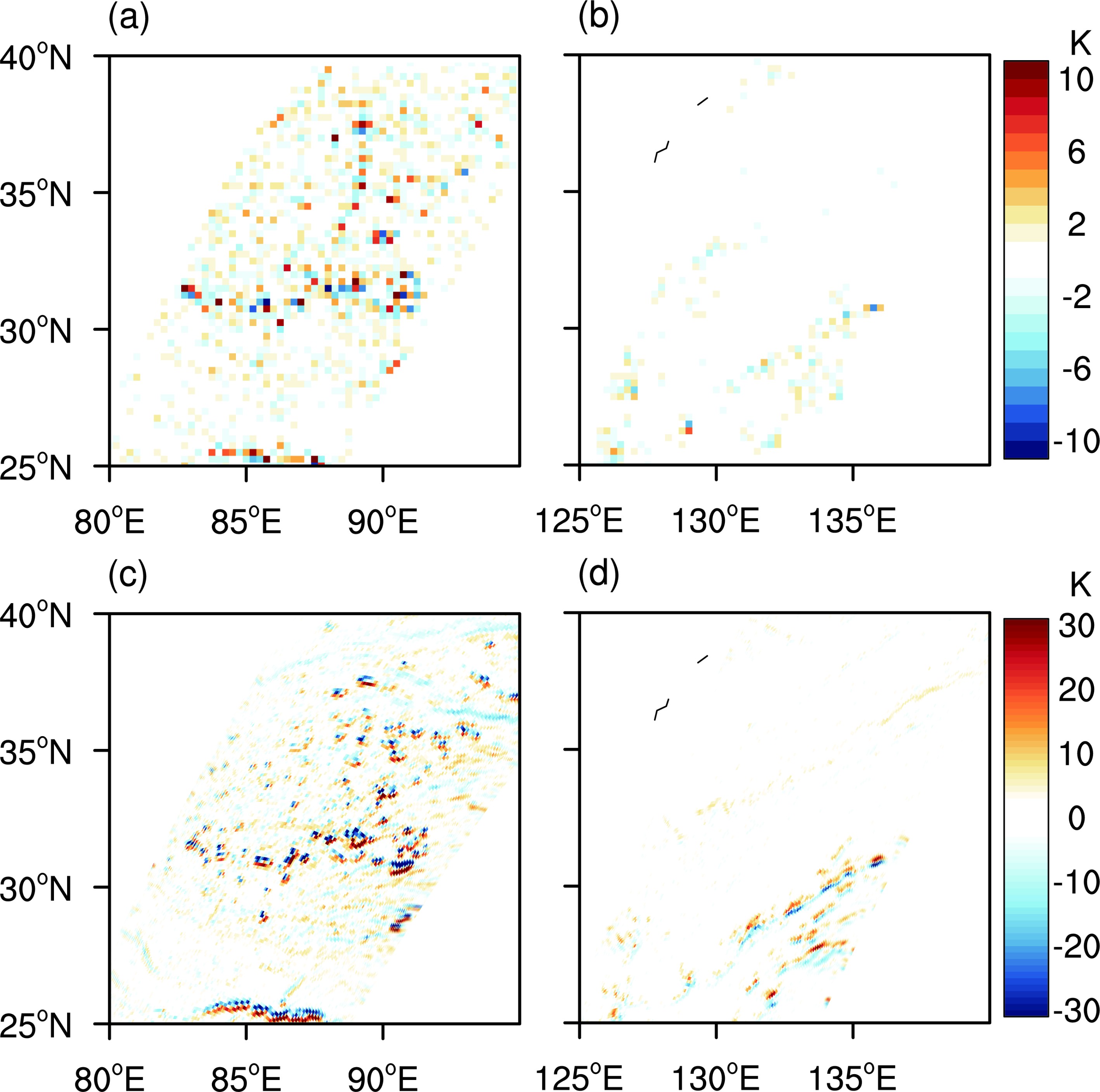Figure11. Differences between the gridded results of the direct and BG methods for two examples: (a) example 1, orbit number 14216; (b) example 2, orbit number 11386. Horizontal distribution of the horizontal gradient of 18.9-GHz V brightness temperature for two examples: (c) example 1, orbit number 14216; (d) example 2, orbit number 11386.

In this paper, the sampling intervals of different regions of the GMI scan line have been analyzed. Three regions on the scan line were computed—namely, the “edge”, “sub-edge” and “center” regions—according to the shortest distance between adjacent pixels. The sampling intervals of the three regions were 6.5 km × 6.0 km, 11.5 km × 6.0 km and 13.0 km × 6.0 km, respectively, which were all smaller than the FOV of the 18.9-GHz channel of GMI (18.1 km × 11.7 km). Therefore, the overlapping parts of the pixels of these three regions were different. Because there were dense overlapping effects between adjacent pixels, overlapping parts had greater weights than others. Furthermore, the FOV of pixels was similar to the size of the 0.25° grid cells; half of the FOVs sampled radiance that lay outside the grid cell, if pixels fell at the grid cell edge. The direct method, which only averages the pixels in the grid cells, caused large errors.
Next, three different sampling intervals of pixels were used to measure the synthesized brightness temperature of a 1000 km × 1000 km area in eastern China. The direct method and BG method were used to process the synthesized brightness temperature of pixels to 25 km × 25 km grid cells. By comparing the results with the true values, it was found that the direct method causes non-negligible errors, especially in regions of large brightness temperature gradient. The error variances between the direct method’s results and the true values were 3.00, 3.62 and 4.99 K² for the three sampling intervals, respectively. Such errors will affect the quality of subsequent retrieval products. To reduce this error, the BG method has been introduced in this paper. The BG method reduces the error of the gridding process by convolving or deconvolving the antenna patterns of pixels onto grid cells’ equivalent antenna patterns. By applying the BG method, the error variance for the three sampling intervals was reduced by about 90%, to 0.22, 0.42 and 0.49 K², respectively. The errors in high brightness temperature gradient regions were also reduced.
Subsequently, the method was applied to real GMI orbits. The results showed that the differences between the results of the BG method and direct method were mainly distributed in the region of large gradients in brightness temperature, which was the same as for the results of the simulation experiment. The results also showed that the BG method can better preserve the information of mesoscale convective systems, cloud boundaries and other regions with large brightness temperature gradients, reduce the error of gridded data, and improve the quality of subsequent retrieval products. However, the BG method also has the disadvantage of high computational expense. As computer hardware evolves, though, the impact of this disadvantage should diminish.
It has been noted that the gridding process can reduce the noise of the instrument itself (Njoku et al., 2003; Deeter and Vivekanandan, 2006). Also, the FOV of the GMI’s 18.9-GHz channel (18.1 km × 11.7 km) is similar to the size of a 0.25° grid cell (25 km), indicating that inversion using the gridded dataset is essentially equivalent to inversion using the pixel. The data processed by the BG method not only reduce the noise of the instrument, but also the error of the gridding process, which is more suitable to inversion. This will be addressed in future research.
Acknowledgements. This study was supported by the National Key R&D Program of China (Grant Nos. 2018YFC1507200 and 2017YFC1501402), the Second Tibetan Plateau Scientific Expedition and Research (STEP) program (Grant No. 2019QZKK0104), an NSFC Project (Grant Nos. 91837310, 41675041, and 41620104009), the Key Research and Development Projects in Anhui Province (Grant No. 201904a07020099), and CLIMATE-TPE (ID 32070) under the framework of the ESA-MOST Dragon 4 program.
Electronic supplementary material: Supplementary material is available in the online version of this article at https://doi.org/10.1007/s00376-021-0358-x.