HTML
--> --> -->The MWTS-2 and MWHS-2 are cross-track radiometers that together provide radiometric information across the 50–60 GHz oxygen band (13 MWTS-2 channels), the 118 GHz oxygen band (8 MWHS-2 channels), the 183 GHz water vapor band (5 MWHS-2 channels), and the atmospheric windows at 89 and 150 GHz (2 MWHS-2 channels). Detailed specifications are provided by He et al. (2015) and Wang and Li (2014). Their combined sounding capability provides sensitivity to temperature from the surface to the upper stratosphere, to humidity throughout the troposphere, and to cloud, precipitation, and surface properties. In some respects, this is similar although not identical to the radiometric capability of the Advanced Microwave Sounding Unit A (AMSU-A) and Microwave Humidity Sounder (MHS), or the Advanced Technology Microwave Sounder (ATMS).
Assessments of MWTS-2 and MWHS-2 have been carried out at the European Centre for Medium Range Weather Forecast (ECMWF) and the Met Office by Lu et al. (2015), Lawrence et al. (2017, 2018), Carminati et al. (2018, 2020), and Duncan and Bormann (2020). These evaluations have been conducted using short-range forecasts from NWP models as a reference comparator as well as a transfer medium for inter-satellite comparisons in double differences. Both techniques are demonstrated by Saunders et al. (2013, 2021).
Prior to its failure in 2015, the MWTS-2 onboard FY-3C was shown to exhibit large cold global biases, scene temperature-dependent biases, scan-dependent biases, cross-track stripping noise, and cross-channel interferences. Feedback from FY-3C assessments helped the China Meteorological Administration (CMA) to mitigate some of these biases on the following instrument thanks to an improved calibration. As a result, the MWTS-2 onboard the FY-3D has significantly improved global biases and virtually no cross-channel interferences, but scan and scene-dependent biases, and striping noise remain similar.
The MWHS-2, onboard both platforms, are operating with a noise level (standard deviation from the short-range forecast departure) comparable to similar instruments at 183 GHz and in line with CMA estimations at 118 GHz (there is no other instrument operating at this frequency for comparison). However, global biases are larger than for the ATMS or MHS at 183 GHz. This has been attributed to the antenna being contaminated by an emissivity leakage. Striping noise, latitude, and scan-dependent biases, not uncommon for this type of instrument, are also present.
Since 2016, several NWP centers, including the Met Office and ECMWF have been assimilating MWHS-2 observations in their operational model (Carminati et al., 2018, 2020; Lawrence et al., 2018; Bormann et al., 2021). The Met Office also has assimilated the observations from MWTS-2 since 2020 (Carminati et al., 2020). Both centers have reported a positive impact on the forecast accuracy and improvement of the background fit to independent instruments.
There is, however, a significant difference in the usage of MWHS-2 data between the Met Office and ECMWF. At the Met Office, only the 183 GHz channels are assimilated and scenes where the atmospheric scattering is non-negligible at this frequency (rain, ice clouds, or deep convection in the field of view) are discarded. The ECMWF system, on the other hand, allows for scattering scenes to be used thanks to a variable observation error that accounts for the presence of cloud in the model background and the observation, as well as an observation operator accounting for atmospheric scattering (Lawrence et al., 2018). This is referred to as all-sky assimilation. Furthermore, some of the 118 GHz channels are also assimilated.
At the Met Office, recent system upgrades (Migliorini et al., 2018) have, for the first time, permitted the usage of microwave observations with scattering-affected scenes (except for rain-induced scattering) which has resulted in a more aggressive use of the AMSU-A (Migliorini and Candy, 2019) and MHS (Candy and Migliorini, 2021) instruments and has improved forecast accuracy. Note that the term all-sky is used here in line with the nomenclature found in these studies, acknowledging that the assimilation of cloud-affected radiances with the exclusion of precipitating scenes does not exploit the full potential of a complete all-sky method. With no technical obstacles to implement this new scheme to other microwave instruments, the all-sky assimilation strategy has been experimented with observations from MWTS-2 and MWHS-2. We anticipate the forecast skills to improve in response to the increased data usage as already demonstrated with AMSU-A and MHS. Additional benefits are also expected from the assimilation of the 118 GHz channels which provide temperature information from 700 to 20 hPa and humidity information in the lower troposphere.
The structure of this document is as follows: section 2 documents the current usage of MWTS-2 and MWHS-2 in the Met Office system and details how their observations are processed within the new all-sky framework, section 3 presents the assimilation experiment set up and discusses the results, and section 4 concludes the study.
Data are then pre-processed, converted to BUFR format, and stored in the Met Office database. The pre-processing is carried out with the Advanced TIROS Operational Vertical Sounder (ATOVS) and the Advanced Very High Resolution Radiometer (AVHRR) Pre-processing Package (
The current operational data assimilation system at the Met Office is a two-stage process, a preliminary one-dimensional variational analysis (1D-Var) followed by the main four-dimensional variational analysis (4D-Var).
The 1D-Var background state is taken from the short-range forecast from the analysis estimated for the previous six-hourly data assimilation cycle, interpolated at each observation location and time. State variables are mapped to radiance space with the fast-radiative transfer model RTTOV version 12 (Saunders et al., 2018). This retrieval scheme is embedded in the observation processing system (OPS) which is designed to control the quality and reduce the number of (or “thin”) the satellite observations that are subsequently used in 4D-Var. Another purpose of the 1D-Var retrieval scheme is to get the best estimate of surface and/or cloud parameters (for example skin temperature and/or cloud top pressure) that are then kept fixed in 4D-Var. Prior to the retrieval, however, observations affected by significant scattering are discarded as further described below.
English et al. (1999) showed that cloud in the field of view can be detected via a cost function of weighted background departures. A combination of thresholds is imposed on the resulting cost and on the magnitude of background departure for certain channels as rejection criteria. In the microwave domain, this test is referred to as mwbcloudy and uses the 183±1, 183±3, and 183±7 GHz channels in the cost function to detect scattering from cirrus clouds. MWTS-2 channels 4 and MWHS-2 channels 13–15 are rejected when scattering is detected. A second scattering test, derived from Bennartz et al. (2002) and referred to as bennartzrain takes advantage of MWHS-2 and MWTS-2 mapping which allows the use of the difference in brightness temperature between the 89 and 150 GHz channels of MWHS-2 which increases in the presence of large hydrometeors or ice particles in the field of view and applies to both instruments. Different thresholds, depending on the surface, are then used to reject observations contaminated by precipitation. MWTS-2 channels 4–7 and MWHS-2 channels 11–15 are rejected when rain or ice is detected via these two tests.
In addition to cloud-based rejection, surface-based rejection criteria are used such that MWTS-2 channel 4 and MWHS-2 channel 15 are rejected over sea ice and land, MWTS-2 channels 5–7 and MWHS-2 channels 11–14 are rejected over sea ice and high land (orography greater than 1000 m), MWTS-2 channel 5 is rejected over land in the tropics, and MWHS-2 channels 11–15 are rejected when the surface to space transmittance exceeds a fixed threshold.
Finally, a common set of quality controls are applied to all the satellite observations processed in OPS. This includes a gross error check on the observation brightness temperature and coordinates (i.e. reject data outside acceptable limits), a gross error check on the background, a convergence check from the 1D-Var, a radiative transfer error check, and a check on background departure before and after the retrieval.
Table 1 summarizes the channel usage and rejection criteria. Note that only MWTS-2 channels 9–13 and MWHS-2 channels 11–15 are used in 4D-Var. The specificities of the assimilation of MWHS-2 in the Met Office regional model are not addressed in this document.
Because the horizontal error correlation is not accounted for in the current error covariance models, observations are thinned such that the data assimilation system uses one observation every 154 km in the tropics and one every 125 km in the extratropics in the cases of both MWTS-2 and MWHS-2.
The successive assimilation stage is a hybrid incremental 4D-Var of dual (N144/N320L70) resolution (Lorenc et al., 2000, 2015; Rawlins et al., 2007). The initial N144 (90 km at mid-latitudes; 70 levels with the model top at 80 km) run performs a Hessian preconditioning aiming at improving the convergence of the higher N320 (40 km at mid-latitudes) resolution run. The system uses a 6-h time window centered on nominal (0, 6, 12, 18 UTC) analysis times. Hereafter, this will be referred to as VAR. The cost function that is minimized in 4D-Var can be written in its generic form as follows:
where x is the guess state, xb the background state, yi the vector of observations, B the background error covariance matrix, R the observation error covariance matrix, Hi the non-linear observation operator, and M the non-linear NWP forecast model integrated from time 0 to time i. The operational forecast model has a N1280L70 resolution (10 km at mid-latitudes; 70 levels with the model top at 80 km). The system is referred to as hybrid when B is flow-dependent, i.e. a contribution to B is derived every cycle from the global ensemble. Finally, in data assimilation theory, y should be bias-free, therefore most satellite radiances are corrected with a variational bias correction model similar to that described by Auligné et al. (2007).
In practice, it is the incremental form of the cost function that is solved. The cost function is, in this case, written as a function of the background departure and solved for the analysis increment (Courtier et al., 1994). This incremental form can be approximated as follows:
with the analysis increment

When focusing on the all-sky data assimilation, the scattering effect induced by hydrometeors needs to be accounted for in the observation operator. RTTOV-SCATT is used to that end as it can simulate the effect of scattering from precipitation in the form of rain or snow and from liquid and ice cloud (Bauer et al., 2006; Saunders et al., 2018, 2020). The parametrization of hydrometeor optical properties is derived from Mie theory (for spherical particles) or the discrete dipole approximation (for a range of non-spherical particles) and is read from lookup tables pre-computed for a range of frequencies, temperatures, and hydrometeor types. Note that in this work both cloud liquid and ice hydrometeors are assumed to be spherical. RTTOV-SCATT works conjointly with the standard RTTOV which simulates the clear part of the atmospheric profiles while RTTOV-SCATT adds the contributions from cloudy radiances.
With the addition of RTTOV-SCATT, the liquid cloud amount ql and ice cloud amount qi can be partitioned from the total water qt control variable in 1D Var, such as:
with qsat the humidity at saturation and fl the ratio between liquid and ice cloud (Candy and Migliorini, 2021). It is therefore possible to retrieve both liquid water path (LWP) and ice water path (IWP). Note that the subsequent hybrid incremental 4D-Var assimilation makes use of a single moist control variable that is nonlinearly related to the specific total water increments so as to be nearly Gaussian distributed (Ingleby et al., 2013). Also, in 4D-Var the partitioning of the total water qt control variable in Eqs. (3) and (4) is replaced by a moisture incrementing operator that partitions the specific total water increments into specific humidity and specific cloud liquid and frozen water increments (Migliorini et al., 2018).
Figure 1 illustrates one model cycle (2020-04-08 1200 UTC) of background departures for FY-3D MWHS-2, 183±1 GHz using all valid data (top), the data with IWP > 0.1 kg m?2 and LWP < 0.05 kg m?2 (middle), and the data with IWP < 0.1 kg m?2 and LWP > 0.05 kg m?2 (bottom). The 1D-Var retrievals reveal the presence of ice and liquid clouds, for example, along a large weather structure across the northern Atlantic (seen as negative departures in the top panel). In this example, bands of ice and liquid clouds, probably from mixed-phase clouds, appear along a southeastward moving front.
The use of RTTOV-SCATT does not prevent the introduction of new systematic errors from assumptions made in the parametrization of the radiative transfer calculation and the misrepresentation of clouds in the model. A common approach to cope with these new biases is to inflate the observation error R on a case-dependent basis. While the Migliorini and Candy (2019) approach for the assimilation of AMSU-A is based on inflating R linearly with the LWP, Candy and Migliorini (2021) showed that it is possible to take advantage of both IWP and LWP such as the observation error, for the ith channel, is defined as:
with

Figure 2 shows the distribution of the standard deviation in the background departures (σOmB) as a function of IWP and LWP for the FY-3D MWTS-2 57.29 ± 0.217 GHz (a), MWHS-2 118.75 ± 2.5 GHz (b), MWHS-2 183.31 ± 1 GHz (c), and MWHS-2 183.31 ± 7 GHz (d) channels (coloured surface). For the low peaking channels, such as 118.75 ± 2.5 GHz (b) or 183.31 ± 7 GHz (d), σOmB grows as expected with the increase of both IWP and LWP, and reaches its largest values (over 2 K) for values of LWP greater than 0.15 kg m?2 and values of IWP greater than 0.40 kg m?2. The blue mesh shows the fit from the least square regression whose coefficients can be used for the calculation of the observation error in Eq. 5. It is important to note, however, that the bilinear regression does not always fit σOmB well, as it can be seen for 57.29 ± 0.217 GHz (a) or 183.31 ± 1 GHz (c). The regression has a poorer fit to σOmB for high peaking channels, as it overestimates σOmB, particularly at high LWP and IWP values, while still providing a conservative observation error standard deviation estimate.
Table 2 summarizes the value of the coefficients from Eq. 5 along with the values of the clear sky error for MWTS-2 and MWHS-2 channels used for operational assimilation. The 1σ standard error is shown in brackets. For stratospheric channels (MWTS-2 9–13 and MWHS-2 2–5), the LWP regression coefficient has been determined to be negative, therefore its value has conservatively been set to zero and a weighted regression recalculated for IWP only. The small dependency of the MWTS-2 stratospheric temperature sounding channels on IWP may however be artificial given system limitations such as suboptimal particle size and shape distribution, mass partitioning of the liquid and ice, and assumptions taken in RTTOV-SCATT. This is further discussed in the next section. Additionally, for MWHS-2 channel 11?12, the IWP coefficients have been determined to be negative, and their values have been recalculated with an unweighted regression of IWP, which avoids giving more weight to bins with lower LWP and IWP values and larger numbers of data points. Note that as a starting point, the clear-sky error standard deviation of the 118 GHz channels has been chosen conservatively large. This will undermine the impact of the temperature-sensitive channels although benefits should still be gained from the improvement of the dynamical initial states. Later work will be dedicated to the optimization of the error standard deviation for these channels.
CRTL is the control experiment. It is configured as a low-resolution version of the operational global system, with the Unified Model producing forecasts at N320L70 UM (~40 km grid length and 70 levels) and the hybrid 4D-Var at N108/N216L70 (~120/~60 km, 70 levels) where the flow-dependent part of the background error is estimated using a N216L70 44-member, 9-hour forecast ensemble. In the control, FY-3C MWHS-2 channels 11–15 and FY-3D MWTS-2 channels 9–13, and MWHS-2 channels 11–15 are assimilated in clear sky.
EXP-1 evaluates the assimilation of FY-3C and D MWHS-2 183 GHz (11–15) channels in all-sky. For this experiment, the cloud tests differ in that channels 13–15 are rejected by the mwbcloudy test over land only (i.e. cloudy observations over the ocean are no longer rejected). RTTOV-SCATT is activated and the observation error can be inflated for channels 11–15 using the coefficients in Table 2. Everything else is the same as in the control.
EXP-2 evaluates the assimilation of FY-3C MWHS-2 183 GHz (11–15) channels and FY-3D MWHS-2 118 (2–7) and 183 GHz (11–15) channels in all-sky. The bennartzrain test rejects channels 2–7 in addition to 11–15 when triggered. The surface to space transmittance test is extended to the lowest peaking 118 GHz channels (5–7). The mwbcloudy test rejects channels 5–7 and 13–15 over land. The observation error is inflated for channels 2–7 and 11–15 using the coefficients in Table 2. Everything else is the same as in the control.
EXP-3 is as EXP-2 except that the observation error is also inflated for MWTS-2 temperature sounding channels 9–13.
EXP-4 is as EXP-2 except that only the channels for which the regression fits the error well (5–7 and 13–15, in green in Table 2) are assimilated in all-sky.
The all-sky assimilation of the 183 GHz channels increases the number of assimilated radiances by 4%, 5%, and 4% at 183.31 ±3.0, ±4.5, and ±7.0 GHz, respectively for FY-3D, and 5.5%, 7%, and 5.5% for FY-3C. This represents about 200 to 500 more radiances per channel at each cycle. The increased number of radiances from these channels is consistent across the four experiments. At 183.31 ±1.0 and ±1.8 GHz, the number of assimilated radiances increase by 1% and 2%, respectively for both platforms across all four experiments. Given that the cloud tests are still active for these channels, their change in observation count results from the background being pulled closer to the observations by the additional information gained from the lower peaking three 183 GHz channels, allowing more data to pass the quality controls. Compared to the control and EXP-1, the use of the 118 GHz channels adds around 9000 new radiances from each of the upper-tropospheric and stratospheric channels (2–4) and around 5000 from each of the tropospheric channels (5–7). There is no significant change in the observation count of the MWTS-2 temperature sounding channels.
Observations (e.g. sondes, aircraft, or surface) and ECMWF operational analyses have been used as independent data sources to evaluate the impact on key forecast variables at lead times from 12 hours to seven days. The overall change in root mean square error (RMSE) in the forecasts is summarized in Table 3. In addition, the fit of independent satellite observations to the background, expressed as the variation of the standard deviation in the background departure, is also analyzed. The latter is a good indication of how the 6-h forecast responds to the changes tested in the experiments and has the advantage of providing a verification against each channel of each instrument used in the data assimilation system.
The differences in the verification against ECMWF analyses (and observations) between EXP-2 to 4 (all including the 118 GHz channels) are marginal, but EXP-4 presents the best overall score and a slightly better observation fit to the background. That the all-sky assimilation of the highest-peaking 118 GHz MWHS-2 channels in EXP-2 and MWTS-2 temperature sounding channels in EXP-3 do not add benefit confirms that these channels have no sensitivity to scattering (mostly because peaking high in the stratosphere where clouds and hydrometeors are rare or non-existent) and supports the idea that IWP sensitivity (i.e. non-null bi coefficients) in MWTS-2 channels is, at least partly, an artifact caused by system sub-optimalities. For the 118 GHz channels, the results are consistent with the work by Chen and Bennartz (2020) that shows no impact of hydrometeor water path and vertically integrated radar reflectivity on the 118.75 ± 0.08, ± 0.2, and ± 0.3 GHz channels.
It is however more surprising to find little differences regarding the all-sky assimilation of the 183 ± 1.0 and ± 1.8 GHz channels as in EXP-2 and EXP-3, and their clear-sky use in EXP-4. With Jacobian peaking, on average, at pressures less than 500 hPa, these channels are less likely to be affected by strong scattering compared to the lower peaking channels. It is possible that the bennartzrain test at these frequencies is too conservative, which could cause mostly clear data to be used in the all-sky scheme, thus suppressing the potential benefit of assimilating scattering scenes. Future work will be dedicated to the retuning of the testing thresholds or its total removal for these two channels, but this is beyond the scope of the present study.
Having determined that neither the all-sky assimilation of the MWHS-2 high peaking 118 GHz channels nor the MWTS-2 temperature-sounding channels yield the best outcome, the rest of the discussion focuses on drawing parallels between the control, EXP-1, and EXP-4.
Figure 3 shows standardized Met Office verification scorecards highlighting the change in RMSE in the forecasts between control and EXP-1 (a) and EXP-4 (b) verified against ECMWF analyses for key atmospheric variables at lead times from 12 to 168 hours. For both experiments, the change in RMSE can be considered to be neutral overall but some patterns can be underlined. Scorecards against observations (not shown) present similar features as described below.
For EXP-1 (Fig. 3a) significant RMSE variations range between –0.69% to +0.71% for an overall change of –0.01%. A persistent degradation (down to –0.2%) of the 2 m temperature in the northern hemisphere (NH_T_2m) is seen for lead times of 12–72 hours. This is balanced by improvements in the tropics (TR_T_2 m, up to +0.1%) and in the southern hemisphere (SH_T_2 m, up to +0.3%). For short lead times, improvements are visible for the southern hemisphere winds (up to +0.3% for SH_W250, SH_W850, and SH_W10 m, representative of the wind at 250 hPa, 850 hPa, and 10 m, respectively) and the temperature at 850 hPa (up to +0.5% for SH_T850). Degradations, on the other hand, seem persistent for 500 and 850 hPa geopotential height (down by –0.6% for SH_Z500 and SH_Z850).
For EXP-4 (Fig. 3b), significant variations of RMSE appear mostly at short lead times and range from –0.34 to +0.88% for an overall change of +0.03%. Similar to EXP-1, the 2 m temperature degrades (down to –0.2%) in the 12–24 forecast lead times while showing neutral changes in the tropics and southern hemisphere. Southern winds also improve (up to +0.3%) from 10 m to 250 hPa. Low-level tropical winds (TR_W10m and TR_W850) slightly degrade (down to –0.2%) between days 3 and 4.
A scorecard comparing the two experiments to each other (rather than to the control) is shown in Fig. 4. Significant differences range from –0.61% to +0.82% with an overall score of +0.04% to the advantage of EXP-4. While there is not much difference in the northern hemisphere, EXP-4 does not capture tropical winds and temperatures as well as EXP-1 but outperforms it in the southern hemisphere. Particularly, there is a persistent improvement (up to +0.6%) of the geopotential height at 850 hPa (SH_Z850) across most lead times and an improvement of all the winds and upper-level temperatures for mid-range lead times. The improvement of southern winds, especially in EXP-4, is likely the signature of the tracer effect described by Geer et al. (2014). The tracer effect is the ability of the adjoint model in 4D-Var to improve dynamical initial states such as wind to better fit the cloudy radiances from humidity-sensitive channels. Unlike the ECMWF however, the Met Office 4D-Var system does not use outer loops (i.e. no multiple updates of the nonlinear forecast during the minimization of the cost function) which lessens the benefits of the tracer effect.
The variation of the standard deviation in the background departures of MetOp B Infrared Atmospheric Sounding Interferometer (IASI) and ATOVS assimilated channels is shown in Fig. 5 for EXP-1 and Fig. 6 for EXP-4. It is expressed as the ratio of the standard deviation in background departure from the experiment divided by that of the control and normalized to 100. Note that IASI channels are referenced by index number as used in the Met Office system and not instrument channel number. Indexes 1–75 are stratospheric temperature sounding channels (wavenumbers 654–706 cm?1), 76–125 are tropospheric temperature sounding channels (707–759 cm?1), 126–135 are lower tropospheric sounding channels sensitive to both temperature and humidity (773–811 cm?1), 136–171 are mostly window channels (833–1206 cm?1), and 172–280 are lower tropospheric humidity sounding channels (1212–1996 cm?1).
The patterns of change for IASI standard deviation are broadly similar in both experiments, that is, a significant reduction for the lowermost temperature sounding channels, most of the sounding channels sensitive to lower tropospheric temperature and humidity, and the humidity sounding channels. The magnitude of the change is however greater for EXP-4, especially for lower tropospheric temperature and humidity sounding channels of indexes in the 112–136 range (744–811 cm?1) with improvements of up to 0.6% compared to up to only 0.3% for EXP-1. The five window channels in the 163–170 index range (1096–1204 cm?1) also improve by up 1.2% for EXP-4 while neutral to detrimental change is visible for EXP-1. Humidity-sounding channels improve in both experiments by up to 0.5%. Similar results have been observed (but are not shown) for the other hyperspectral instruments in the system (MetOp C IASI, SNPP CrIS, NOAA20 CrIS, and Aqua AIRS).
ATOVS assimilated channels, composed of AMSU-A channels 4–6 and 8–14, and MHS channels 3–5, see a consistent improvement of both the stratospheric temperature sounding channels (AMSU-A 12–14) and the tropospheric humidity sounding channels (MHS 3–5). This is also observed for the ATOVS on board all the platforms used in the system (NOAA15, NOAA18, NOAA19, and MetOp C). EXP-1 has a slightly better impact than EXP-4 on MHS humidity-sounding channels, with improvements of up to 0.3% (and up to 0.7% for MHS onboard NOAA19, not shown). The largest gain for the AMSU-A stratospheric temperature sounding channels is obtained through EXP-4, up to 0.5%. There is a small 0.1% degradation in EXP-4 for AMSU-A channel 10 peaking around 50 hPa. This is detected for the instruments onboard MetOp B and NOAA19. The ATMS stratospheric temperature sounding channels (12–15) deteriorate consistently across all experiments (not shown) by 0.1 to 0.5% (maximum for channel 14) and therefore unaffected by the assimilation of the 118 GHz channels. It is not clear what causes ATMS degradation but the vicinity of NOAA20, SNPP, and FY-3D orbits may play a role, i.e. create an effect similar to an increase of observation count that statistically results in an increased standard deviation.
The microwave temperature and humidity sounders onboard the Chinese platforms of the FY-3 series, presenting characteristics close to the ATOVS systems plus a unique set of channels sounding the 118 GHz oxygen band, have become the next logical candidate for the all-sky radiance assimilation. In addition to the potential benefit from a more aggressive use of available observations, insights into the added value of the 118 GHz channels can guide the applications related to future satellite missions such as the Microwave Imager (MWI) onboard MetOp-SG platforms or the Cubesats constellation TROPICS (Time-Resolved Observations of Precipitation structure and storm Intensity with a Constellation of Smallsats) supported by the NASA Earth Venture-Instrument (EVI-3) program.
Several set-ups have been tested in which radiances from MWTS-2 and MWHS-2 were assimilated in all-sky (except precipitating scenes). The configuration in which MWHS-2 high peaking 118.75 ± 0.08, ±0.2 and ±0.3 GHz, and 183.31 ± 1 and ±1.8 GHz channels are assimilated with a fixed observation error while the low peaking 118.75 ± 0.8, ±1.1 and ±2.5 GHz, and 183.31 ± 3.0, ±4.5 and ±7.0 GHz are assimilated with a variable observation error has yielded the best impact. The variable observation errors for these channels vary with the retrieved values of LWP and IWP derived from the Met Office 1D-Var observation processing system.
The verification against ECMWF analyses for key atmospheric variables at different forecast lead times highlights small but significant short-range improvements regarding southern hemispheric winds and low-level temperature balanced by some degradation of short-range northern and tropical low-level temperatures. The overall impact is neutral.
A detailed examination of the short-range forecasts shows an improvement of the observation fit to the background across the microwave and the infrared spectral domains. The use of the all-sky assimilation methodology for MWHS-2 183 GHz channels alone yields up to 0.4% improvement for IASI lower tropospheric humidity and temperature sounding channels, and up to 0.3% improvement for both AMSU-A stratospheric temperature sounding channels and MHS humidity sounding channels. The MWHS-2 highest humidity sounding channels 183.31 ± 1.0 and 183.31 ± 1.8 GHz, however, does not add significant benefit when used in all-sky (while increasing the computational cost through the use of RTTOV-SCATT) for the configuration tested in this study. The relaxing of the bennartzrain scattering test may let more cloudy radiances into the assimilation system and drive further benefits. This will be subject to investigation for a future model upgrade.
The additional assimilation of five 118 GHz channels (118.75 ± 0.08, ±0.2, ±0.3, ±0.8, ±1.1, and ± 2.5 GHz), including three in all-sky (118.75 ± 0.8, ±1.1, and ±2.5 GHz) further improves the fit to the background of most instruments assimilated in the system. The improvement reaches 1.2% for IASI low peaking temperature sounding channels and 0.5% for AMSU-A stratospheric temperature sounding channels. The combination of temperature and humidity sensitivity of the 118.75 ± 2.5 GHz appears particularly effective in improving the IASI fit to the background in the 773–811 cm?1 and 1096–1204 cm?1 spectral ranges.
Pending further verifications, such as high-resolution assimilation experiments, the all-sky assimilation of MWHS-2 radiances at 118 and 183 GHz is a candidate for future implementation in the Met Office system.
| Channel | Weighting function peaking pressure (hPa) | Frequency (GHz) | Usage |
| MWTS-2 | |||
| 1 | 1050 | 50.30 QH | Used for gross error checks only |
| 2 | 1050 | 51.76 QH | Used for gross error checks only |
| 3 | 962 | 52.80 QH | Used for gross error checks only |
| 4 | 661 | 53.596 ± 0.115 QH | Rejected when mwbcloudy and bennartzrain Rejected over sea ice and land Used in 1D-Var only |
| 5 | 410 | 54.40 QH | Rejected when bennartzrain Rejected over sea ice and highland (and land in the tropics) Used in 1D-Var only |
| 6 | 300 | 54.94 QH | Rejected when bennartzrain Rejected over sea ice and highland Used in 1D-Var only |
| 7 | 181 | 55.50 QH | Rejected when bennartzrain Rejected over sea ice and highland Used in 1D-Var only |
| 8 | 97 | 57.29 QH | Used in 1D-Var only |
| 9 | 55 | 57.29 ± 0.217 QH | Used in 1D-Var and 4D-Var |
| 10 | 29 | 57.29 ± 0.3222 ± 0.048 QH | Used in 1D-Var and 4D-Var |
| 11 | 10 | 57.29 ± 0.3222 ± 0.022 QH | Used in 1D-Var and 4D-Var |
| 12 | 4 | 57.29 ± 0.3222 ± 0.010 QH | Used in 1D-Var and 4D-Var |
| 13 | 2 | 57.29 ± 0.3222 ± 0.0045 QH | Used in 1D-Var and 4D-Var |
| MWHS-2 | |||
| 1 | 1050 | 89.0 QH | Used for gross error checks only |
| 2 | 25 | 118.75 ± 0.08 QV | Not used |
| 3 | 55 | 118.75 ± 0.2 QV | Not used |
| 4 | 97 | 118.75 ± 0.3 QV | Not used |
| 5 | 236 | 118.75 ± 0.8 QV | Not used |
| 6 | 372 | 118.75 ± 1.1 QV | Not used |
| 7 | 1033 | 118.75 ± 2.5 QV | Not used |
| 8 | 1033 | 118.75 ± 3.0 QV | Not used |
| 9 | 1050 | 118.75 ± 5.0 QV | Not used |
| 10 | 1033 | 150 QH | Used for gross error checks only |
| 11 | 491 | 183.31 ± 1 QV | Rejected when bennartzrain Rejected over sea ice and highland Rejected when surface to space transmittance > 0.15 Used in 1D-Var and 4D-Var |
| 12 | 533 | 183.31 ± 1.8 QV | Rejected when bennartzrain Rejected over sea ice and highland Rejected when surface to space transmittance > 0.15 Used in 1D-Var and 4D-Var |
| 13 | 618 | 183.31 ± 3.0 QV | Rejected when mwbcloudy and bennartzrain Rejected over sea ice and highland Rejected when surface to space transmittance > 0.15 Used in 1D-Var and 4D-Var |
| 14 | 704 | 183.31 ± 4.5 QV | Rejected when mwbcloudy and bennartzrain Rejected over sea ice and highland Rejected when surface to space transmittance > 0.15 Used in 1D-Var and 4D-Var |
| 15 | 826 | 183.31 ± 7.0 QV | Rejected when mwbcloudy and bennartzrain Rejected over sea ice and land Rejected when surface to space transmittance > 0.15 Used in 1D-Var and 4D-Var |
| Note: QV: quasi-vertical; QH: quasi-horizontal; QC: quality control. | |||
Table1. Summary of MWTS-2 and MWHS-2 channel usage and rejection criteria. Weighting function peaking pressure has been calculated with RTTOV 54-level coefficients, at nadir, for the U.S. standard atmosphere, and rounded to the nearest hPa.
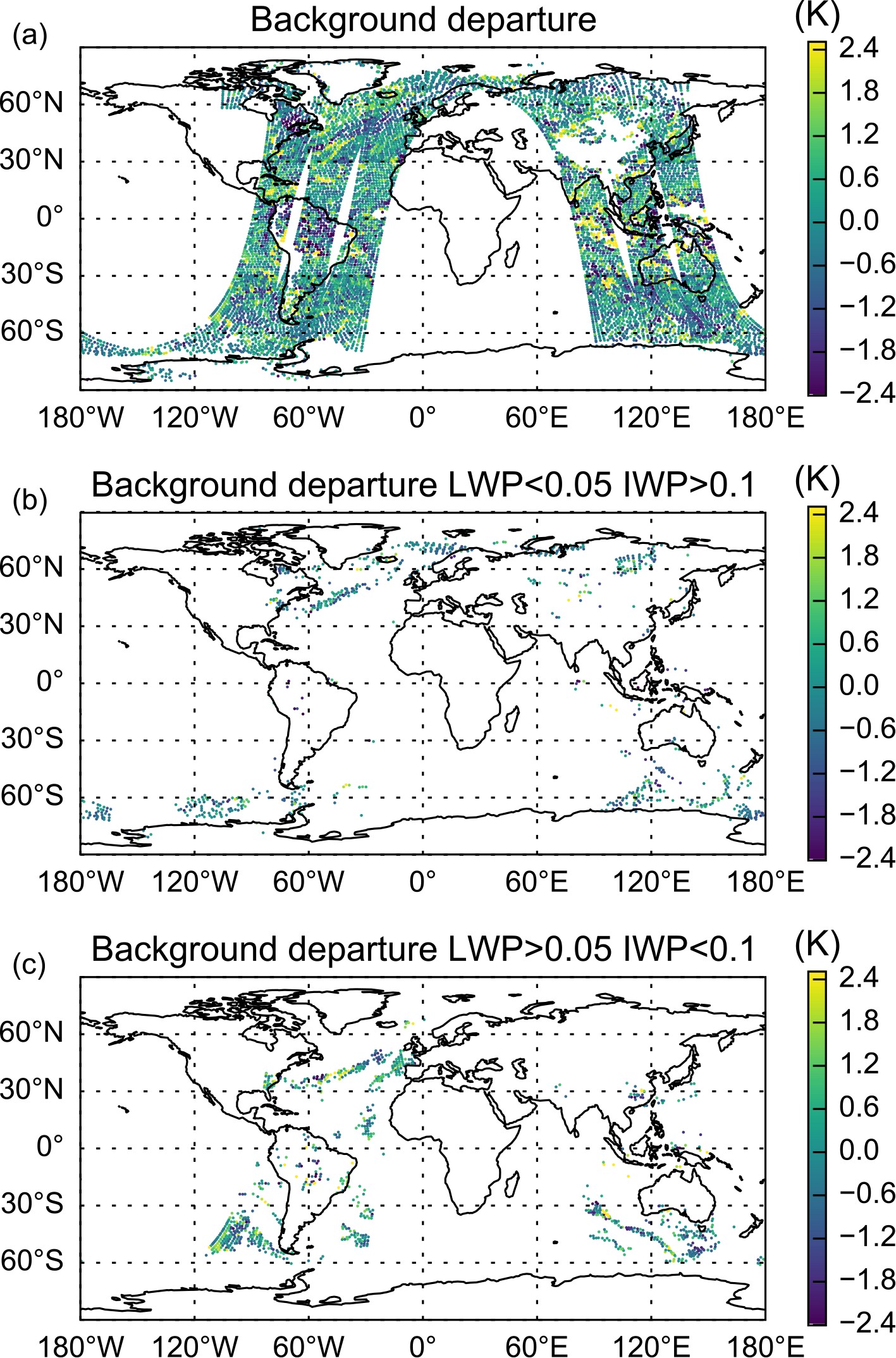 Figure1. FY-3D MWHS-2 183 ± 1 GHz background departures (K) on 1200 UTC 8 April 2020. (a) panel shows all valid data including scattering scenes, (b) panel shows the data where LWP is less than 0.05 kg m?2 and IWP greater than 0.1 kg m?2, i.e. mainly of ice cloud, and (c) panel shows the data where LWP is greater than 0.05 kg m?2 and IWP less than 0.1 kg m?2, i.e. mainly liquid cloud.
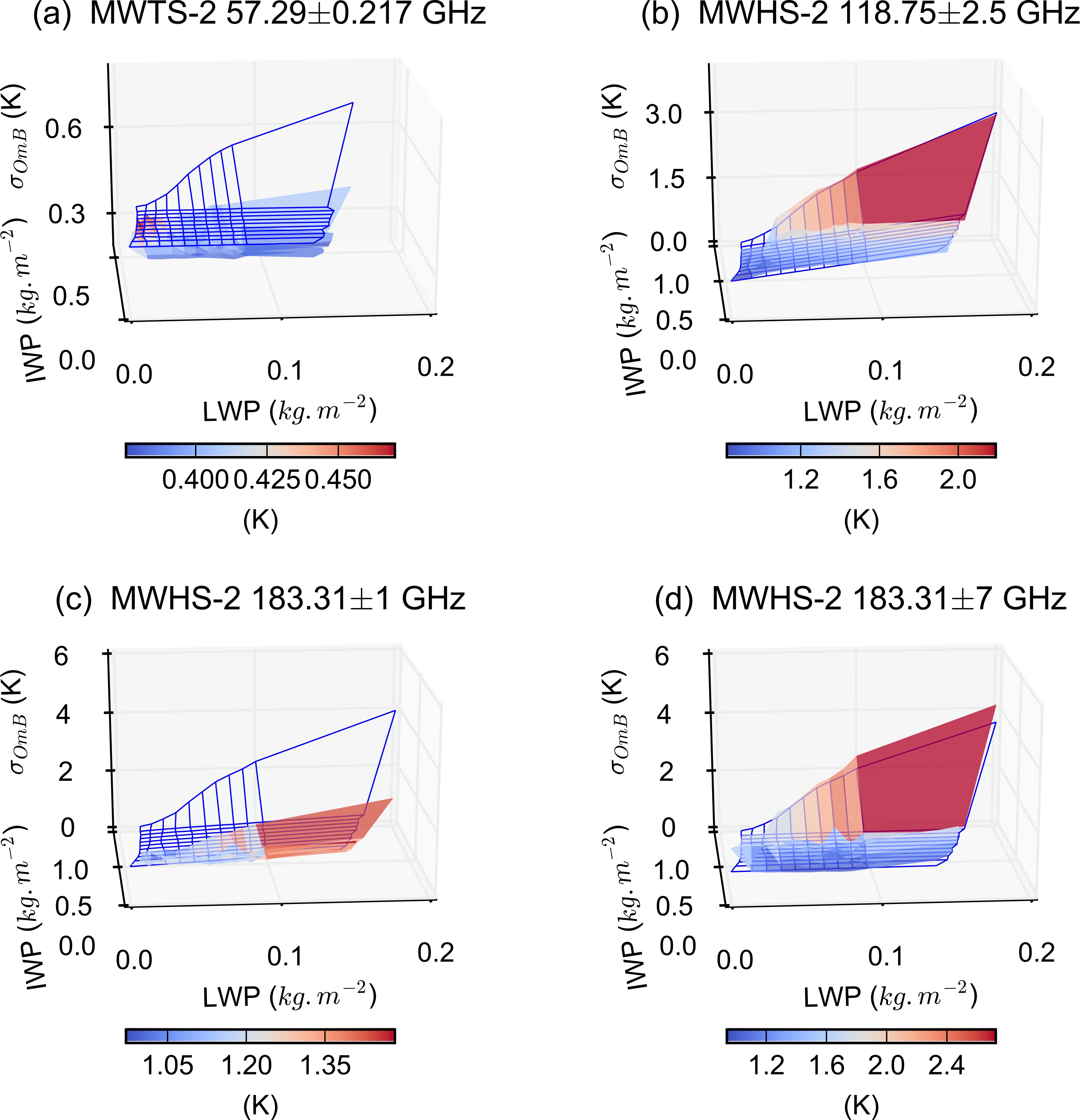 Figure2. Observation error standard deviation for (a) MWTS-2 57.29 ± 0.217 GHz, (b) MWHS-2 118.75 ± 2.5 GHz, (c) MWHS-2 183.31 ± 1 GHz, and (d) MWHS-2 183.31 ± 7 GHz as a function of LWP and IWP. The colored contour shows the standard deviation in the background departure and the blue mesh shows the fit from the least square regression.
| Channel number & frequency (GHz) | $ \sigma _i^{{\rm{clr}}} $ (K) | ai (±1σ) (K kg?1 m2) | bi (±1σ) (K kg?1 m2) |
| MWTS-2 | |||
| 9 (57.29±0.217) | 0.7300 | 0 | 0.5306 (0.1438) |
| 10 (57.29±0.217±0.048) | 1.3100 | 0 | 0.4196 (0.1095) |
| 11 (57.29±0.217±0.022) | 1.3700 | 0 | 0.5023 (0.0741) |
| 12 (57.29±0.217±0.010) | 2.3200 | 0 | 0.3123 (0.0691) |
| 13 (57.29±0.217±0.0045) | 4.7900 | 0 | 0.1282 (0.0315) |
| MWHS-2 | |||
| 2 (118.75±0.08) | 4.0000 | 0 | 0.3942 (0.0935) |
| 3 (118.75±0.2) | 3.0000 | 0 | 0.2762 (0.0496) |
| 4 (118.75±0.3) | 3.0000 | 0 | 0.1009 (0.0288) |
| 5 (118.75±0.8) | 4.0000 | 0 | 0.3959 (0.0581) |
| 6 (118.75±1.1) | 4.0000 | 0.0166 (0.0410) | 0.5973 (0.0216) |
| 7 (118.75±2.5) | 4.0000 | 3.9740 (0.1506) | 3.1724 (0.0875) |
| 11 (183.31±1) | 2.8028 | 2.8780 (0.3799) | 0.0529 (0.0912) |
| 12 (183.31±1.8) | 2.6230 | 2.3057 (0.2904) | 4.0106 (2.1055) |
| 13 (183.31±3.0) | 1.7717 | 1.9393 (0.2877) | 0.8576 (0.1243) |
| 14 (183.31±4.5) | 1.9913 | 1.3075 (0.2939) | 2.3607 (0.1585) |
| 15 (183.31±7.0) | 1.9981 | 0.2561 (0.3291) | 5.4332 (0.2487) |
Table2. Clear-sky observation error standard deviation and regression coefficients (with the coefficient 1σ standard error in brackets) for the MWTS-2 and MWHS-2 channels assimilated in VAR. The values in bold show the channels for which the least square regression fits reasonably well with the standard deviation in O-B from the training set.
| RMSE (%) change against observations | RMSE (%) change against ECMWF analyses | |
| EXP-1 vs CRTL | 0.03 | ?0.01 |
| EXP-2 vs CRTL | 0.01 | ?0.05 |
| EXP-3 vs CRTL | 0.05 | ?0.03 |
| EXP-4 vs CRTL | 0.12 | 0.03 |
| EXP-4 vs EXP-1 | 0.09 | 0.04 |
Table3. Summary of the overall RMSE (%) change against observations (left) and against ECMWF analyses (right) for EXP-1 to -4 vs. CRTL and for EXP-4 vs. EXP-1.
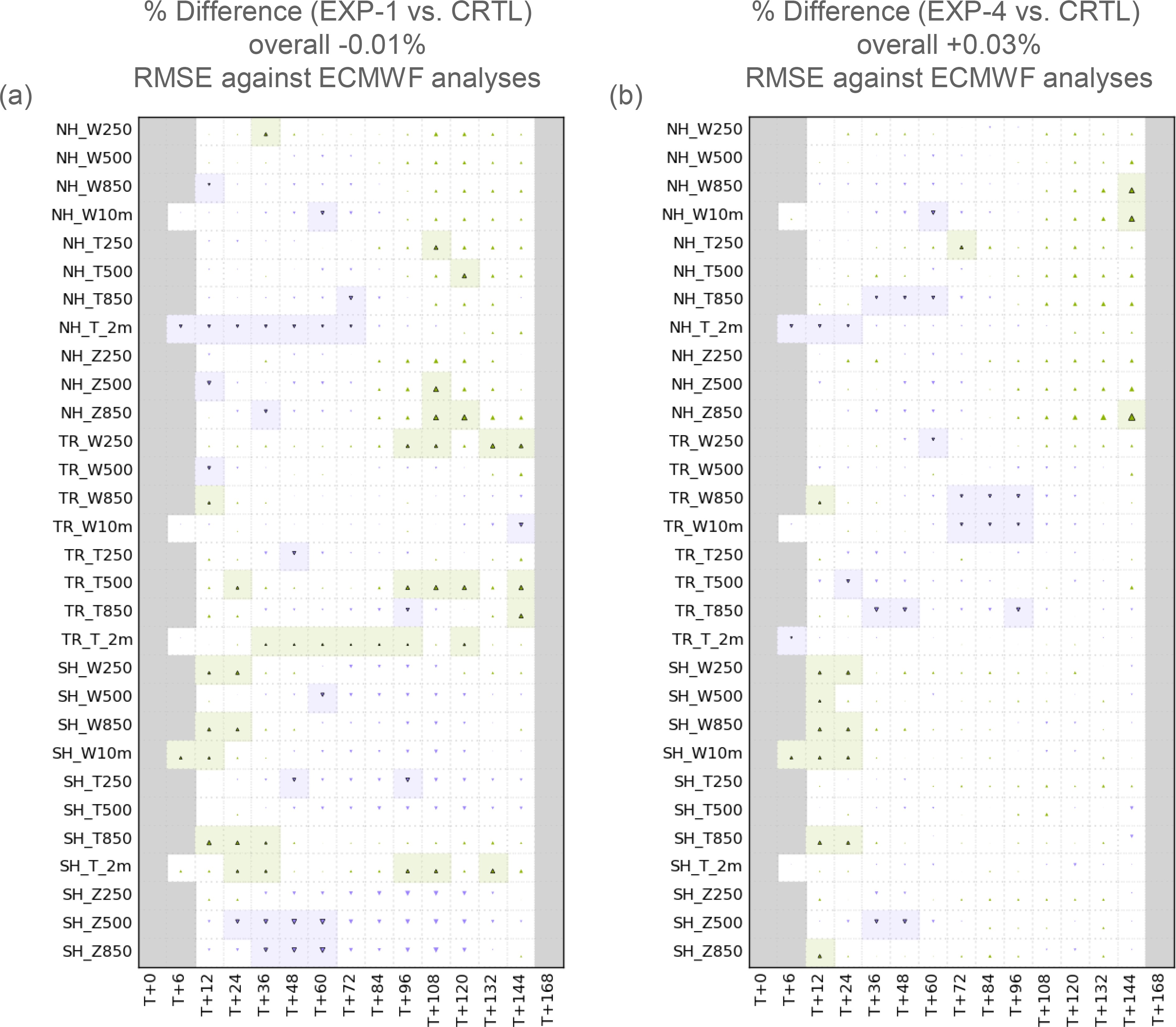 Figure3. Change in the root-mean-square forecast error between EXP-1 (a), EXP-4 (b), and the control for key atmospheric variables at lead times from T+6 to T+168 with respect to the ECMWF analyses. Triangle color, size, and direction are given by 100 x (control RMSE–trial RMSE) / control RMSE. Upward green indicates that the trial RMSE is smaller than the control RMSE. Downward purple indicates that the trial RMSE is larger than the control RMSE. Significance is given by shading.
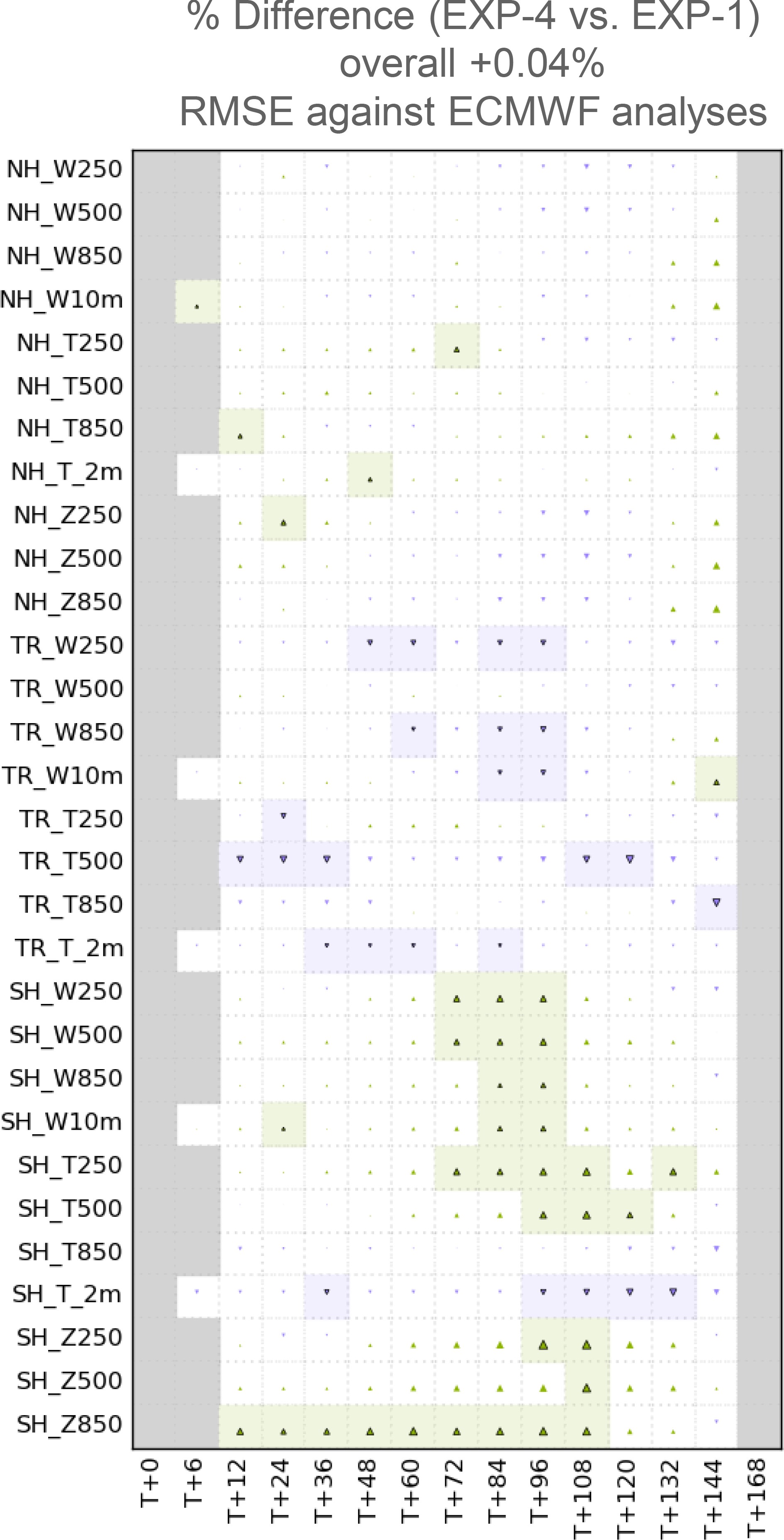 Figure4. RMSE difference between EXP-4 and EXP-1 with respect to the ECMWF analyses.
 Figure5. Change in standard deviation in the background departure for MetOp B IASI (a) and MetOp B ATOVS (b) in EXP-1. Red indicates a significant increase, green a significant decrease, and blue no significant change. The numbers at the top of each plot indicate the mean change across all channels (±1σ).
 Figure6. Same as Fig. 5 but for EXP-4.
Acknowledgements. This work was supported by the UK – China Research & Innovation Partnership Fund through the Met Office Climate Science for Service Partnership (CSSP) China as part of the Newton Fund. We are grateful to Chawn HARLOW for the useful discussions that helped us improve this study.
Open Access This article is distributed under the terms of the Creative Commons Attribution 4.0 International License (
