The First Global Carbon Dioxide Flux Map Derived from TanSat Measurements

HTML

--> --> -->

1. Introduction

Top-down carbon flux inversion by assimilating atmospheric carbon dioxide (CO₂) measurements is a useful tool for evaluating the global carbon budget and was used in the 2019 Refinement to the 2006 Intergovernmental Panel on Climate Change (IPCC) Guidelines for National Greenhouse Gas Inventories. Ground-based measurements provide highly accurate continuous data and have improved our understanding of global carbon flux. However, the sparseness and spatial inhomogeneity of the existing ground-based network limits our ability to infer consistent global- and regional-scale CO₂ sources and sinks (Scholes et al., 2009), especially for tropical and high-latitude regions.
To improve observation coverage, tailor-made satellites have been developed to provide atmospheric greenhouse gas (GHG) measurements at unprecedented precision. The Japanese GHG monitoring satellite mission, Greenhouse Gases Observing Satellite (GOSAT), was launched in 2009 (Kuze et al., 2009), and the U.S. satellite mission, Orbiting Carbon Observatory 2 (OCO-2), was launched in 2014 (Crisp et al., 2017).
Satellite measurements are advantageous for constraining top-down flux inversions because they provide continuous global observation coverage. Although satellite measurements are not as accurate as ground-based measurements, the increased spatial coverage can provide additional information not available from sparse surface networks (Buchwitz et al., 2007), and such data have been used in surface carbon flux inversion studies (Peylin et al., 2013; Saeki et al., 2013; Jiang et al., 2016; Chevallier et al., 2019; Wang et al., 2020). The CO₂ column-averaged dry-air mole fractions (XCO₂) measured by GOSAT and OCO-2 have been applied in regional carbon flux optimization studies (Basu et al., 2013; Maksyutov et al., 2013; Feng et al., 2017; Chevallier et al., 2019; Wang et al., 2020).
Recent studies have shown that the accuracy of inversion results inferred from the GOSAT and OCO-2 retrievals is comparable to traditional inversions using accurate but sparse surface networks, indicating that satellite GHG observations provide valuable complementary data for global carbon budget studies (Chevallier et al., 2019; Wang et al., 2020). Assimilation of satellite GHG observations has significantly changed or raised questions about our understanding of spatiotemporal patterns of surface CO₂ fluxes. For example, GOSAT inversion data suggest high European biospheric uptake, nearly twice that suggested by in situ-only studies (Houweling et al., 2015; Feng et al., 2016; Reuter et al., 2017), which would modify the global carbon flux distribution (Houweling et al., 2015). Assimilated GOSAT and OCO-2 XCO₂ measurements have also revealed unexpectedly high net emissions from tropical Africa, which are thought to be mainly caused by substantial land-use change, resulting in the release of carbon from large soil organic carbon stores (Palmer et al., 2019).
The Chinese Global Carbon Dioxide Monitoring Scientific Experimental Satellite (TanSat), funded by the Ministry of Science and Technology of China, the Chinese Academy of Sciences, and the China Meteorological Administration, was launched in December 2016 (Liu and Yang, 2016; Ran et al., 2019). The first global XCO₂ map measured by TanSat was reported in a previous study (Yang et al., 2018), and Total Column Carbon Observing Network validation shows 2.2 ppm accuracy for version 1 of the TanSat L2 data product (Liu et al., 2018). The accuracy and precision of TanSat XCO₂ retrievals were further improved using a wavelength dependence gain factor to correct the spectrum continuum feature (Yang et al., 2020). A new version of TanSat XCO₂ was recently released to the public (Yang et al., 2021), which provides an opportunity to improve our knowledge of global carbon flux from flux inversions based on TanSat measurements.
In this study, we introduce the first estimate of global carbon flux based on TanSat global measurements. The following section shows the TanSat measurements and methods used in the flux inversion. Section 3 introduces the main results of the optimized carbon flux. We then close with our conclusions.

2. Method

2.1. TanSat measurement

-->

2.1. TanSat measurement

TanSat flies in a sun-synchronous low Earth orbit (LEO) with an equator crossing time around 1330 local time and operates in three observation modes including nadir (ND), glint (GL), and target modes. ND mode is used when TanSat flies over land surfaces, and GL mode is activated over the ocean to increase the incident signal and ensure the signal-to-noise ratios meet the requirements. The atmospheric carbon dioxide grating spectrometer on board TanSat provides hyperspectral measurements of the O₂ A band (0.76 μm) and CO₂ weak (1.61 μm) and strong (2.04 μm) bands. The ND footprint size of TanSat measurement is ~2 × 2 km with nine footprints across the track in a frame, while the total field-of-view width is ~18 km. The TanSat repeat measurement cycle is 16 days, and the ND and GL measurements are staggered. In ND mode, TanSat has the same ground track interval as OCO-2.
XCO₂ retrieval is performed using the Institute of Atmospheric Physics carbon dioxide retrieval algorithm for satellite remote sensing (Liu et al., 2013; Yang et al., 2015). The version 1 TanSat XCO₂ retrievals only used the CO₂ weak band due to calibration issues on the O₂ A band (which can cause critically biased estimates of surface pressure). Therefore, the flux inversion precision and accuracy were not adequate for studying global surface carbon flux. Further study on solar calibration measurements revealed a remaining feature on the solar spectrum fitting residual. A Fourier series model was applied as a gain factor to the continuum in the retrieval, significantly improving the fitting residual, especially on the O₂ A band. The O₂ A band and CO₂ weak band measurements have been used together in new retrievals that correct the parameters of water vapor, surface pressure, temperature, aerosol, cirrus, and instrument model. A genetic algorithm was used in post screening, and then a multiple linear regression model was applied to correct bias (Yang et al., 2020). In this study, we used a 15-month (March 2017–May 2018) XCO₂ retrieval from TanSat ND measurements.
Only “good” retrievals have been provided in the TanSat v2 product used in flux inversion. We used single sounding uncertainty (posterior error) to construct weighted time–space average data (Crowell et al., 2019). First, we calculated a 1-second span average:
where $ {X}_{{{\rm{C}}{\rm{O}}}_{2},i} $

is the ith sounding value in a 1-second span with a total of N soundings, and $ {\sigma }_{i} $

is the corresponding posterior error. The summary includes all soundings in a 1-second span, and the uncertainty for the 1-second average is:
where we assumed soundings in a 1-second span were highly correlated. Because the posterior error mainly considered the theoretical error from the measurement noise level, the $ \overline {{\sigma }_{1{\rm{s}},\sigma }} $

estimation was sometimes lower than real measurement uncertainty. Therefore, we also considered the standard deviation $ \overline {{\sigma }_{1{\rm{s}},{\rm{s}}{\rm{t}}{\rm{d}}}} $

; the uncertainty of a 1-second span, $ \overline {{\sigma }_{1{\rm{s}}}} $

, was the maximum of either $ \overline {{\sigma }_{1{\rm{s}},\sigma }} $

or $ \overline {{\sigma }_{1{\rm{s}},{\rm{s}}{\rm{t}}{\rm{d}}}} $

. This differs from the 1-second spans of OCO-2 because TanSat L2 sounding values have not been corrected for the bias of small areas. Thus, small systematic uncertainty, such as floor error, was not considered.
In this study, we used a 5-second span average for flux inversion. The $ \overline {{X}_{{{\rm{C}}{\rm{O}}}_{2},5{\rm{s}}}} $

and $ \overline {{\sigma }_{5{\rm{s}}}} $

values were constructed using the methods for 1-second spans of sounding measurements.

2

2.2. Carbon flux inversion system

-->

2.2. Carbon flux inversion system

We used an ensemble transform Kalman filter (ETKF) data assimilation system (Feng et al., 2009, 2011, 2016) to estimate global and regional carbon flux. The carbon flux and CO₂ concentration were optimized by TanSat XCO₂ measurements via:
where ${{x}}^{{\rm{a}}}$

and ${{x}}^{{\rm{f}}}$

are the a posteriori and a priori fluxes, respectively. H_oo is the observation operator that describes the relationship between the state vector and the observations. $ {{y}}_{{\rm{o}}{\rm{b}}{\rm{s}}} $

is XCO₂ measured by TanSat, and K is the Kalman gain matrix, which determines the adjustment to the a priori based on the difference between the model and observations and their uncertainties as follows:
where R is the observation error covariance matrix, namely, a diagonal matrix representing measurement errors, including instrument error, retrieval error, model error, and representation error (Peylin et al., 2002). ${{P}}^{{\rm{f}}}$

is the a priori error covariance matrix. The Jacobian of the observation operator, H, maps ${{P}}^{{\rm{f}}}$

into observation space. In our carbon flux inversion system, we used the chemistry transport model (CTM) GEOS-Chem (v9-02) in forward simulation [$H\left({{x}}^{{\rm{f}}}\right)$

] and performed an ensemble run to establish the connection between surface fluxes and atmospheric CO₂ concentrations (H).
We used sequentially assimilated TanSat 5-second averaged measurements day by day in each assimilation step (1 month) to optimize the a priori estimation of surface CO₂ fluxes. The GEOS-5 meteorological analyses, provided by the NASA Goddard Global Modelling and Assimilation Office, were used to drive the GEOS-Chem run. The model was run at a horizontal resolution of 4° (latitude) × 5° (longitude) with 47 vertical levels, which spanned from the surface to the mesosphere, typically with 35 levels in the troposphere. Monthly inventories have been used as the a priori flux for GEOS-Chem runs, including ocean flux (Takahashi et al., 2009), biomass burning fluxes (van der Werf et al., 2010), 3-hourly terrestrial biosphere fluxes (Olsen, 2004), and fossil fuel emissions (Oda and Maksyutov, 2011). For the terrestrial biosphere, we used a 3-hour flux to better represent and optimize the uptakes and emissions from photosynthesis and respiration processes, respectively (Olsen, 2004). The inversion for surface flux spanned 792 regions globally, including 475 land regions and 317 ocean regions, based on a TransCom 3 study (Gurney et al., 2002).

3. Results

3.1. Annually integrated global carbon net flux

-->

3.1. Annually integrated global carbon net flux

In this study, only the ND model land observations were applied to constrain the flux optimization. Due to the low signal-to-noise ratio, the ND measurements over the ocean are not provided in the L2 XCO₂ data product, and no further information is provided by TanSat ocean measurements. Therefore, a very strong prior constraint was applied to the ocean CO₂ flux. The inversion result is shown as carbon flux based on CO₂ flux using the mass ratio between CO₂ and carbon.
Error reduction for global carbon sinks indicates how well the measurements optimized the estimations. The error reduction in July was greater than in other months (Fig. 1); for example, it was > 50% in northern Asia, Europe, and America, but lower in Australia, southern Asia, and India. South America and Africa showed 20%–40% error reduction. TanSat measurements improved results in South Africa mostly in April and October, in North and South America mostly in July, and in northern Eurasia in all three months.

Figure1. The reductions in uncertainty for (a) July 2017, (b) October 2017, (c) January 2018, and (d) April 2018.

The global annual carbon sinks (Fig. 2) constrained by TanSat measurements differed significantly from a priori fluxes. For example, the land sink increased in most of Northern Asia, Europe, and the Americas, but decreased in the middle of Africa and India. Similar results have been reported in GOSAT and OCO-2 CO₂ flux inversion studies (Wang et al., 2019, 2020). The land sink also increased in southwest China, which is consistent with carbon flux estimations based on additional ground-based in-situ measurements from Asia (Wang et al., 2020). The optimization was not significant over the ocean because no direct measurements were used to constrain the oceanic carbon flux.

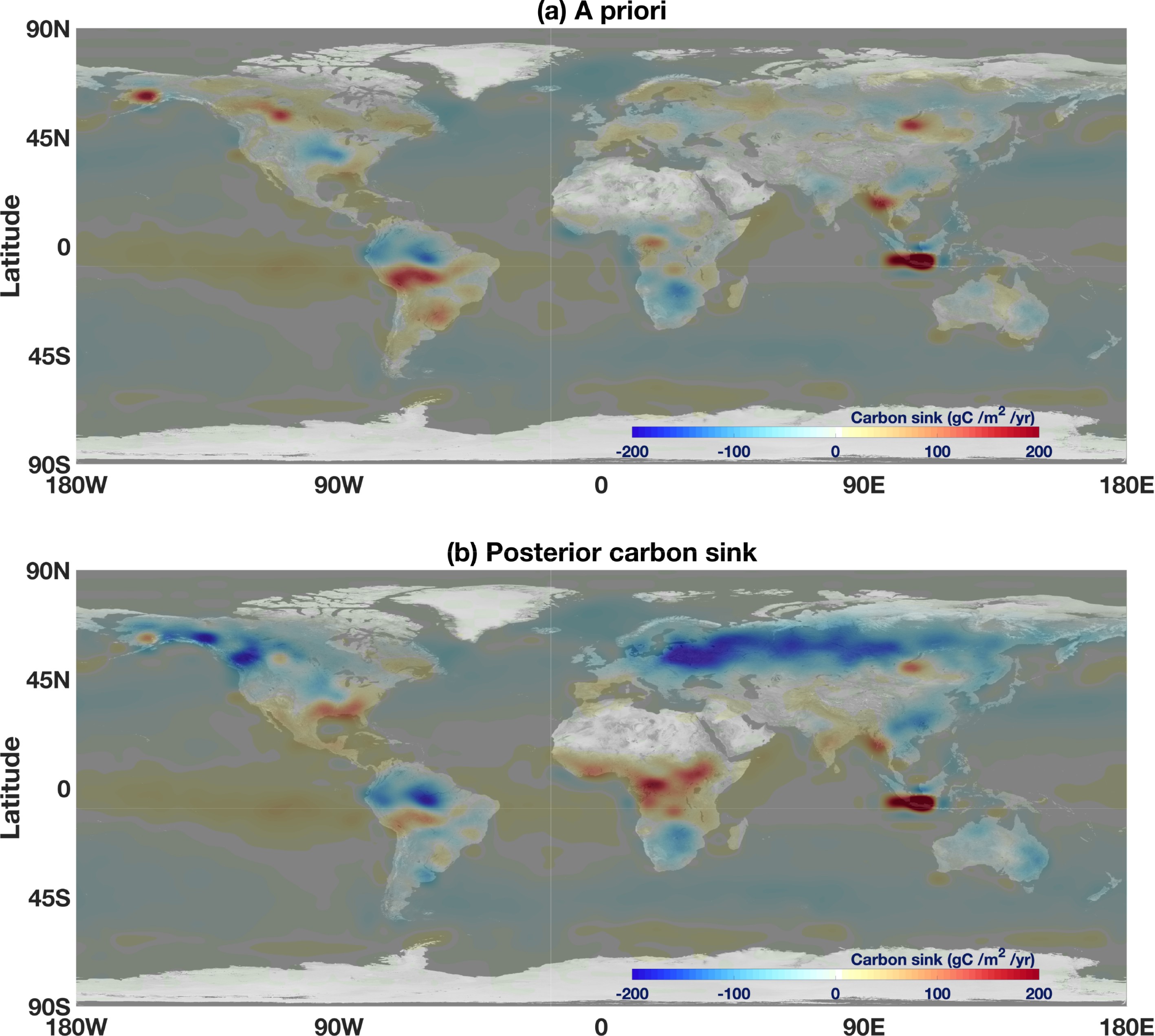Figure2. The annual carbon sink optimized by GOSAT measurements (b) from a priori estimates (a). The color bar indicates the carbon sink.

Our TanSat inversion indicated a land net flux integrated over 12 months (May 2017–April 2018) of 6.71 Gt C yr^?1 with an uncertainty of 0.76 Gt C yr^?1. Table 1 shows the land carbon net flux over the same period constrained by the new L2 OCO-2 XCO2 data product (v10) as a reference. The annul integrated OCO-2 net carbon flux was 5.13 ± 0.59 Gt C yr^?1, which is 23.5% lower than the TanSat results. Several studies have reported different carbon flux estimations based on satellite measurements for 2009 onwards. The GOSAT measurement was the first spaced-based GHG measurement used in global CO₂ flux estimation (Basu et al., 2013). GOSAT measurements indicated land net carbon fluxes estimated by the carbon tracker (Peters et al., 2007; https://www.esrl.noaa.gov/gmd/ccgg/carbontracker/) of 7.86 ± 1.26 Gt C yr^?1 in 2017 and 7.61 ± 1.78 Gt C yr^?1 in 2018. The OCO-2 model intercomparison project showed 10 inversion model parallel studies with results ranging from 5.75 to 8.97 Gt C yr^?1 from June 2017 to May 2018.

Region	A priori		TanSat		OCO-2
Region	Flux	1-σ	Flux	1-σ	Flux	1-σ
North American Boreal (NAB)	0.17	0.33	?0.82	0.19	?0.23	0.19
North American Temperate (NAT)	1.52	0.58	1.53	0.29	1.62	0.27
South American Tropical (SAT)	0.094	0.40	0.78	0.26	0.09	0.22
South American Temperate (SAM)	0.49	0.39	0.065	0.26	?0.76	0.20
North Africa (NAF)	0.20	0.24	1.059	0.18	0.81	0.15
South Africa (SAF)	?0.057	0.44	0.74	0.25	?0.19	0.18
Eurasia Boreal (EAB)	0.10	0.60	?1.12	0.23	?0.12	0.25
Eurasia Temperate (EAT)	3.83	0.42	3.68	0.24	2.89	0.22
Tropical Asia (TA)	1.23	0.27	0.90	0.20	0.61	0.16
Australia (AUS)	0.069	0.20	?0.21	0.17	?0.056	0.15
Europe (EU)	1.15	0.66	?0.18	0.30	0.18	0.28
North land (NL)	6.78	1.43	3.10	0.52	4.34	0.41
South land (SL)	0.50	0.62	0.60	0.38	?1.00	0.30
Tropical land (TL)	1.52	0.54	2.73	0.36	1.51	0.30
Global Land	9.08	1.74	6.71	0.77	5.13	0.59

Table1. The a priori and a posteriori fluxes estimated by TanSat (v2) and OCO-2 (v10) for 11 TransCom regions and continents.

2

3.2. Seasonal and regional CO₂ flux

-->

3.2. Seasonal and regional CO₂ flux

Seasonal net carbon flux was grouped every three months and denoted following the Northern Hemisphere seasons, namely, summer (June, July, August), autumn (September, October, November), winter (December, January, February), and spring (March, April, May). The distribution of global carbon flux differed significantly from a priori flux after assimilation of TanSat measurements (Fig. 3). For example, the measurements (satellite data) significantly changed carbon fluxes for South America for the whole year (Fig. 4). The South America tropical region showed the largest impacts from TanSat measurements, with the seasonal phase shifted significantly from a priori fluxes. We found that the satellite did not provide dense measurements over tropical South America, but even a small amount of TanSat data can still significantly change the carbon flux feature. TanSat measurements increased carbon sinks in spring and summer around Eurasia, including in Europe and boreal and temperate Eurasia, compared with a priori fluxes. North Africa also showed significant increases in the carbon sink in winter. In addition, the seasonal variation of India decreased during spring and summer.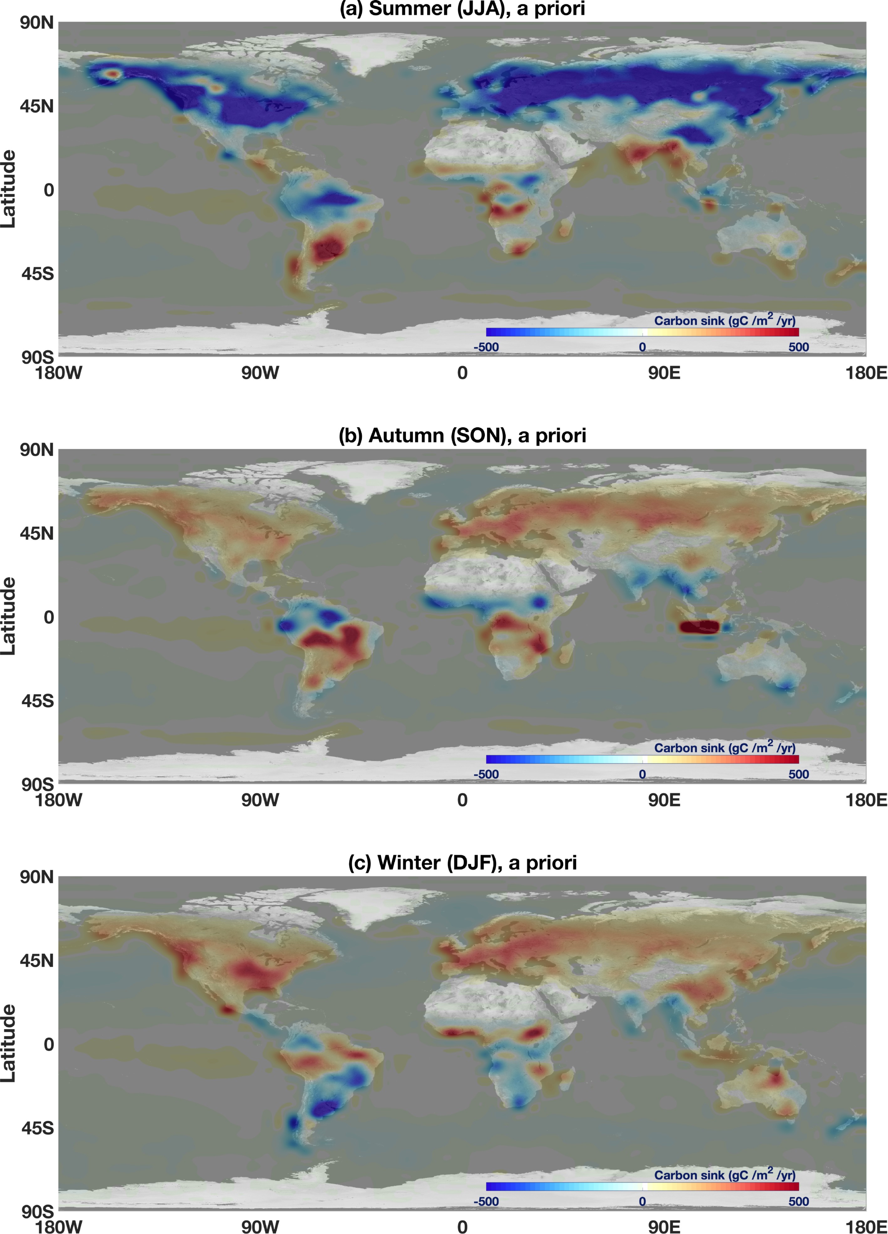

Figure3. The a priori (upper row) and a posteriori (lower row) seasonal carbon sinks constrained by TanSat measurements. The columns indicate summer, autumn, winter, and spring from left to right.

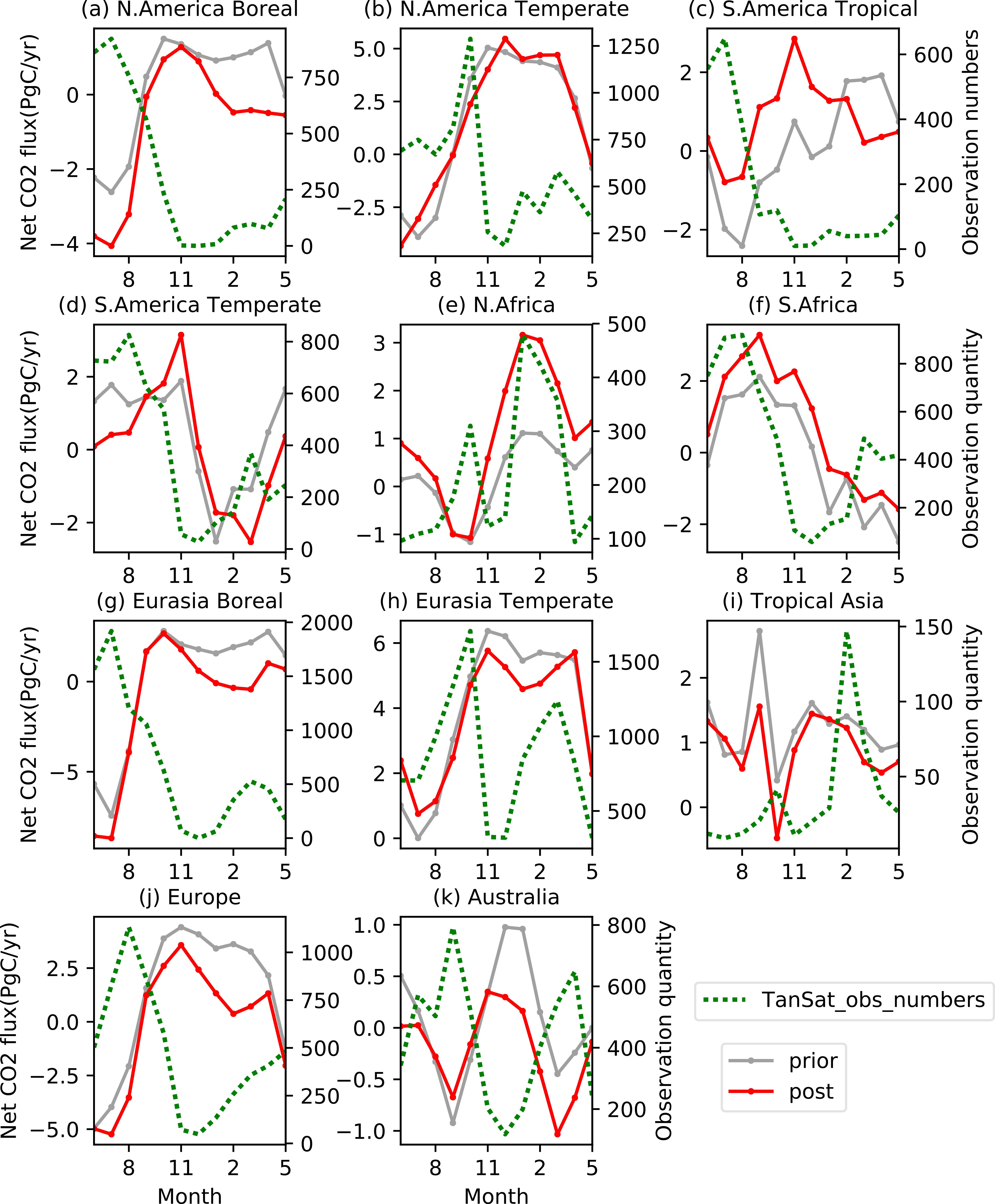Figure4. The a priori and a posteriori CO₂ flux trends for 11 TransCom land regions shown with measurement quantities. The names at the top of each subplot indicate regions.

We also observed changes in China’s carbon flux in autumn, winter, and spring; in general, the carbon sink increased compared to a priori fluxes, especially in southwest China in the summer and autumn. Similar results have been reported by studies of vegetation trend measurements (Chen et al., 2019) and flux estimations (Wang et al., 2020).
Figure 5 shows regional carbon flux from OCO-2 and TanSat measurements, as well as a priori fluxes. OCO-2 and TanSat have similar optimization effects on a priori fluxes in most regions. The biggest discrepancy was in the Southern Hemisphere, where TanSat measurements and a priori fluxes indicated a source, whereas OCO-2 measurements indicated a sink; the difference in outcomes was driven in large part by results from tropical and temperate South America. This contradiction has also been reported when comparing results from GOSAT and OCO-2 measurements (Wang et al., 2019).

Figure5. The carbon flux estimated by TanSat and OCO-2 measurements and the a priori flux in 11 TransCom land regions, South Land (SL), North Land (NL), and globally.

4. Conclusions and outlook

We described the first attempt at estimating global carbon flux using TanSat XCO₂ measurements. We used an ETKF data assimilation system coupled with the GEOS-Chem CTM in a top-down carbon flux inversion. The error reduction compared to a priori estimates demonstrated the impact of assimilating global satellite XCO₂ measurements, which resulted in significant changes in spatiotemporal flux patterns throughout the year from May 2017 to April 2018. Our TanSat inversion indicated an annual integrated global land carbon net flux of 6.71 ± 0.76 Gt C yr^?1, compared to annual totals of 5.75–8.97 Gt C yr^?1 for inversions based on OCO-2 XCO₂ data.
These carbon flux data are publicly accessible worldwide on the China GEO TanSat data service archive, the Cooperation on the Analysis of Carbon Satellites Data (CASA; www.chinageoss.org/tansat), which is hosted by the International Reanalysis Cooperation on Carbon Satellites Data (IRCSD).
TanSat provides preliminary global measurements that extend the ground-based network from local measurements to global estimates. However, the coverage, repeat, pixel size, and accuracy of measurements are still inadequate to meet the Global Stocktake of the Paris Agreement and inventory validation requirements of IPCC standards. For example, GOSAT measurements have indicated that flux estimation is sensitive to measurement coverage (Deng et al., 2014). XCO₂ measurements are also sensitive to regional flux inversion (Feng et al., 2009; Palmer et al., 2011). The future European Copernicus Carbon Dioxide Monitoring satellite mission (Kuhlmann et al., 2019) will improve measurements of global coverage and investigations of anthropogenic emissions. The plan for the next TanSat mission has been discussed and is in the design phase. One possibility is a multi-satellite LEO constellation. Several satellites would capture global background measurements with large pixel size and a wide swath, while others would focus on target measurements for city and point sources with a small pixel size. This would capture carbon sinks and sources at multiple scales to elucidate the influences of natural processes and anthropogenic activities on the carbon cycle.
Column CO₂ measurements are still inadequate for separating local carbon exchanges from long-range transport processes because the signal is mixed into the column value (Keppel-Aleks et al., 2011). The signal of local flux is critical to city and point-source research. Ground-based measurements near the surface will be helpful for future investigations. Therefore, coordinating satellites and surface measurement networks will significantly improve the study of small-scale anthropogenic emission sources.
Acknowledgements. This work is supported by the National Key R&D Program of China (Grant No. 2016YFA0600203), the Key Research Program of the Chinese Academy of Sciences (ZDRW-ZS-2019-1), the National Key R&D Program of China (Grant No. 2017YFB0504000), and the Youth Program of the National Natural Science Foundation of China (Grant No. 41905029). Liang FENG is supported by the UK NERC National Centre for Earth Observation (NCEO). The TanSat L1B data service is provided by IRCSD and CASA (131211KYSB20180002). We also thank the FENGYUN Satellite Data Center of the National Satellite Meteorological Center, who provided the TanSat L1B data service. The authors thank the TanSat mission and highly appreciate the support from everyone involved.

本站小编 Free考研考试/2022-01-02

Corresponding author: Jing WANG,jingwang@mail.iap.ac.cn;

HTML

2.1. TanSat measurement

2.2. Carbon flux inversion system

3.1. Annually integrated global carbon net flux

3.2. Seasonal and regional CO₂ flux

相关话题/First Global Carbon

领限时大额优惠券,享本站正版考研考试资料!

A Positivity-preserving Conservative Semi-Lagrangian Multi-moment Global Transport Model on the Cube

The First Fengyun Satellite International User Conference

Analysis of the Effect of Optical Properties of Black Carbon on Ozone in an Urban Environment at the

Natural Climate Solutions for China: The Last Mile to Carbon Neutrality

Global Freshwater Storage Capability across Time Scales in the GRACE Satellite Era

The Assessment of Global Surface Temperature Change from 1850s: The C-LSAT2.0 Ensemble and the CMST-

Characteristics of Lake Breezes and Their Impacts on Energy and Carbon Fluxes in Mountainous Areas

A New Global Solar-induced Chlorophyll Fluorescence (SIF) Data Product from TanSat Measurements

Future Changes in Extreme High Temperature over China at 1.5°C–5°C Global Warming Based on CMIP6 Sim

A New TanSat XCO<sub>2</sub> Global Product towards Climate Studies