HTML
--> --> -->CMIP is designed to better understand past, present, and future climate change from unforced natural variability or in response to radiative forcing changes through multi-model simulations (Eyring et al., 2016). The CMIP historical simulations are an indispensable part of the entry card for participating CMIP6. They start from arbitrary equilibrium conditions from the pre-industrial control experiment (piControl) and integrate with time-dependent observational forcing, including greenhouse gas (GHG) emissions (for ESMs) or concentrations (for CSMs), land-use forcing, anthropogenic aerosols, stratospheric aerosols (volcanoes), solar forcing, and ozone concentrations and nitrogen deposition etc. Therefore, the historical simulations can serve as the benchmark of model performance as these simulations can be validated against the observational records. The change in global mean surface temperature from pre-industrial times to the present day in the historical simulations, as well as their spatial characteristics, are critical metrics of the model performance, which directly determine the reliability of the future climate projection produced by the model. In China, the development of global climate models began in the 1980s and great achievements have been made in the past 40 years, including the involvement in every CMIP phase (Zhou et al., 2020).
In recent years, a climate system model known as CAMS-CSM was developed at the Chinese Academy of Meteorological Sciences (Rong et al., 2018). The performance of the early version of CAMS-CSM has been fully evaluated, including the climatology and seasonal cycle (Rong et al., 2018), climate sensitivity (Chen et al., 2019), intraseasonal variability (Qi et al., 2019; Ren et al., 2019; Wang et al., 2019), El Ni?o–Southern Oscillation (ENSO) and the teleconnections (Hua et al., 2019; Lu and Ren, 2019), annular modes (Nan et al., 2019), land heat and water (Zhang et al., 2018), and so on. Based on these evaluation, a couple of updates have been made for CAMS-CSM to improve its simulation of cloud radiative forcing and radiation transfer. This new version of CAMS-CSM is the one that is running the formal CMIP6 simulations. At the time of writing, CAMS-CSM has completed all the entry card simulations of CMIP6, and the model outputs have been published onto the Earth System Grid Federation (ESGF) data server (
This paper is arranged as follows: Section 2 presents a brief introduction to the CMIP6 version of CAMS-CSM and the design of its historical experiments. Section 3 describes the technical detail of the model output datasets. Section 4 presents some basic validation of the outputs from the historical simulations. Finally, usage notes are provided in section 5.
2.1. Model
The configuration of the CAMS-CSM version used for CMIP6 simulations is described in in detail in the paper by Rong et al. (2018). Here, to facilitate the users of the CAMS-CSM historical simulation datasets, we again provide an introduction to the model.The atmospheric component of CAMS-CSM is a modified version of ECHAM5(v5.4) (Roeckner et al., 2003). The resolution adopted for the CMIP6 historical simulations is T106 L31, which indicates a resolution of approximately 1° horizontally with 31 vertical levels. The top of the atmospheric model is 10 hPa. The major modifications of the CAMS-CSM version to the original ECHAM5 model include: (i) a two-step shape-preserving advection scheme for the water vapor advection (Yu, 1994; Zhang et al., 2013); and (ii) a correlated k-distribution scheme with the Monte Carlo Independent Column Approximations developed by Zhang et al. (2003, 2006a, b) for the calculation of radiation transfer. There are two differences between the CMIP6 version and the early version used in Rong et al. (2018): (i) a modification of the conversion rate from cloud water to precipitation in the cumulus convection scheme (from 2 × 10?4 m?1 to 1 × 10?4 m?1), which is able to improve the cloud radiative forcing simulation (Zhang et al., 2020); and (ii) an effective solar zenith angle scheme accounting for the curvature of the atmosphere and its effect on the length of the optical path of the direct solar beam with respect to a plane parallel atmosphere.
The ocean component is the Geophysical Fluid Dynamics Laboratory (GFDL) Modular Ocean Model, version 4 (MOM4) (Griffies et al., 2004). The horizontal resolution is fixed to 1° zonally, with a variable meridional resolution: 1/3° within 10°S–10°N, which increases to 1° at 30°S and 30°N, and a nominal 1° in the bipolar Artic region poleward of 60°N for the tripolar grid. MOM4 employs a Z vertical coordinate that contains 50 vertical levels, with 23 even levels placed above 230 m to better represent the thermocline. The subgrid physical parameterization configured for the historical simulations is the same as Rong et al. (2018), which includes: an anisotropic Laplacian scheme for horizontal viscosity; isoneutral diffusion for tracers; K-Profile Parameterization together with Bryan–Lewis vertical diffusion/viscosity schemes; tidal mixing, overflow for dense water crossing steep bottom topography; full convective adjustment scheme; and solar penetration with climatological chlorophyll concentration etc.
The sea-ice component is the GFDL Sea Ice Simulator (SIS) (Winton, 2000), using the same grid as the ocean model. SIS is a thermodynamic/dynamic sea-ice model. It adopts a three-layer structure: one snow layer and two sea-ice layers of equal thickness. In each grid there are five categories of sea ice and one open-water area. The different categories’ sea ice is redistributed based on an enthalpy conserving approach. The elastic–viscous–plastic technique developed by Hunke and Dukowicz (1997) is employed for calculation of the internal ice stresses.
The Common Land Model (CoLM) (Dai et al., 2003) is utilized as the land component, using the same grid as the atmospheric model. In CoLM, each surface grid cell is comprised of up to 24 land-cover types. The soil is divided exponentially into 10 unequal vertical layers, with a thickness of 1.75 cm for the top layer and 114 cm for the bottom layer. A two-big-leaf submodel is employed in CoLM for photosynthesis, stomatal conductance, leaf temperature, and energy fluxes (Dai et al., 2004). The CAMS-CSM version implements an unfrozen water process (Niu and Yang, 2006) that allows liquid water to remain in the soil when the temperature is below 0°C.
CAMS-CSM uses the GFDL Flexible Modelling System coupler for calculation of fluxes/states and interpolations among component models. For stability and efficiency considerations, a new conservative coupling algorithm has been developed to guarantee the implicit treatment of the air–ice fluxes as well as a low communication cost among component models (Rong et al., 2018).
2
2.2. Experiment designs
We conducted three historical simulation experiments for CAMS-CSM (Table 1). The first experiment “r1i1p1f1” starts from the initial conditions of 1 January 3025 of the piControl experiment. The external forcing used for this simulation is from the recommendation of CMIP6 (https://esgf-node.llnl.gov/projects/input4mips), which includes historical GHG concentrations (CO2, CH4, N2O, CFC-12, and equivalent CFC-11, accounting for the radiative effects of all 39 other gases) (Meinshausen et al., 2017), ozone concentrations (| Experiment_id | Variant_label | Integration time | Experiment design |
| historical | r1i1p1f1 | 1850–2014 | Starts from 1 January 3025 of the piControl experiment. The external forcing includes historical GHGs (CO2, CH4, N2O, CFC-12, and equivalent CFC-11), ozone concentrations, stratospheric aerosols, the total solar irradiance, and anthropogenic aerosols. Land-use forcing is fixed in this simulation. |
| historical | r2i1p1f1 | 1850–2014 | Same as r1i1p1f1, but starts from 1 January 3030 of the piControl experiment. |
| historical | r1i1p1f2 | 1850–2014 | Same as r1i1p1f1, but excludes the stratospheric aerosol forcing. |
Table1. Experiment designs.
Monthly mean and daily mean outputs are provided for the CAMS-CSM datasets. There are 38 monthly mean variables for the atmospheric model dataset, including air temperature, humidity, velocity, sea level pressure, precipitation, radiation fluxes, surface heat fluxes and momentum fluxes, cloud water and cloud ice, cloud cover, etc. In total, 11 monthly mean variables of the oceanic model are provided, including sea temperature, salinity, velocity, surface heat flux, mixed-layer depth, sea surface height etc. The monthly mean outputs of the land model contain 10 variables, including soil temperature, soil moisture and ice, evaporation, etc. The sea-ice model provides 18 monthly mean variables, including sea-ice concentration, temperature, velocity, thickness, sea ice transport, surface stress, surface snow thickness, etc. The daily mean outputs are provided only for the atmospheric model, which contain 15 variables including air temperature, velocity, humidity, surface temperature, precipitation, radiative fluxes, etc.
2
4.1. Climatology of temperature, precipitation and sea ice
We first examine two fundamental metrics for coupled climate model performance: climatological annual mean surface air temperature and precipitation. Figure 1 shows the simulated and observed surface air temperature climatology. It can be seen that the model reproduces the global distribution of surface air temperature reasonably well. The overall spatial pattern of the simulated surface air temperature resembles that from the observations. Over much of the ocean and terrestrial areas, the biases are less than 1°C [globally averaged bias is ?0.145°C, and the root-mean-square error (RMSE) is 2.42°C]. Evident biases primarily lie in the North Atlantic and the Southern Ocean near the Antarctic, where the biases can be larger than 5°C (with a significance level of 5%). The cold biases over the high latitudes of the North Atlantic are associated with the overestimated sea-ice cover in the Northern Hemisphere, while the warm biases near the Antarctic might be ascribed to the underestimated sea-ice extent over there. In the eastern coastal regions of the tropical Pacific and Atlantic, the simulated surface temperature tends to be warmer than observed, which is a usual feature of coupled climate models and may result from their inadequate representation of stratocumulus and coastal upwelling. We also calculated the surface air temperature error over land using CRUTEM4 data. The result shows that the global mean biases and RMSE over land are ?0.128°C and 2.14°C, respectively, which are smaller than those of the previous version (?1.53°C and 2.31°C), suggesting a performance improvement in the CMIP6 version.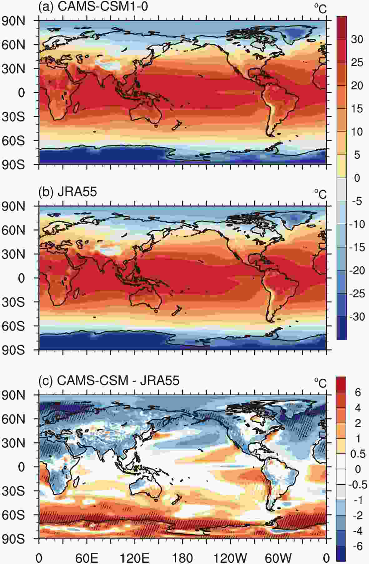 Figure1. The climatology (1980–2014-averaged) of surface air temperature at 2 m: (a) ensemble mean of CAMS-CSM historical simulations (r1i1p1f1 and r2i1p1f1); (b) JRA-55 data; (c) differences between CAMS-CSM historical simulations and JRA-55 data. The hatched areas in the plots denote the significance level of 5% from the t-test against the interannual anomalies. Units: °C.
Figure 2 shows the simulated and observed annual mean precipitation. Overall, the simulated precipitation shows a similar pattern to the observations (globally averaged bias of 0.03 mm d?1; RMSE of 1.15 mm d?1). The active precipitation centers, such as the intertropical convergence zone (ITCZ), South Pacific convergence zone (SPCZ), and South Atlantic convergence zone (SACZ), as well as those over the tropical Indian Ocean and subtropical oceans, are reasonably captured by the model. Compared with the GPCP data, the simulated precipitation over the tropical oceans is generally overestimated, especially over the areas of the ITCZ and SPCZ, where the biases can exceed 4 mm d?1 and the general precipitation pattern in the tropical Pacific tends to bear a double-ITCZ structure. To some extent, the double-ITCZ bias is improved compared with the previous version (Rong et al., 2018); however, it still remains a prominent discrepancy of the CAMS-CSM model. Although it is recognized that the double-ITCZ errors arise from the Bjerknes feedback between atmosphere and ocean, how to eliminate this bias remains unresolved and the double-ITCZ still stands out as a prevailing error in current coupled models (Zhang et al., 2015). Notably, the double-ITCZ bias has been largely reduced in the FGOALS-f3-L model (Guo et al., 2020), possibly benefiting from the convection scheme adopted in the model, and suggesting that improving physical schemes might be an effective way to eliminate the double-ITCZ error. Over the tropical Atlantic, the simulated SACZ shifts southward to the warm SST bias area, with excessive precipitation in the tropical South Atlantic. Dry biases can be found in the central and eastern equatorial Pacific, as a result of an overestimated cold tongue in the model. A certain connection exists between the temperature biases and precipitation biases over some land areas. For example, the warm biases over tropical Africa and the Amazon appear to be associated with the dryer biases over these regions, while the cold biases over the Tibetan Plateau correspond to overestimated precipitation.
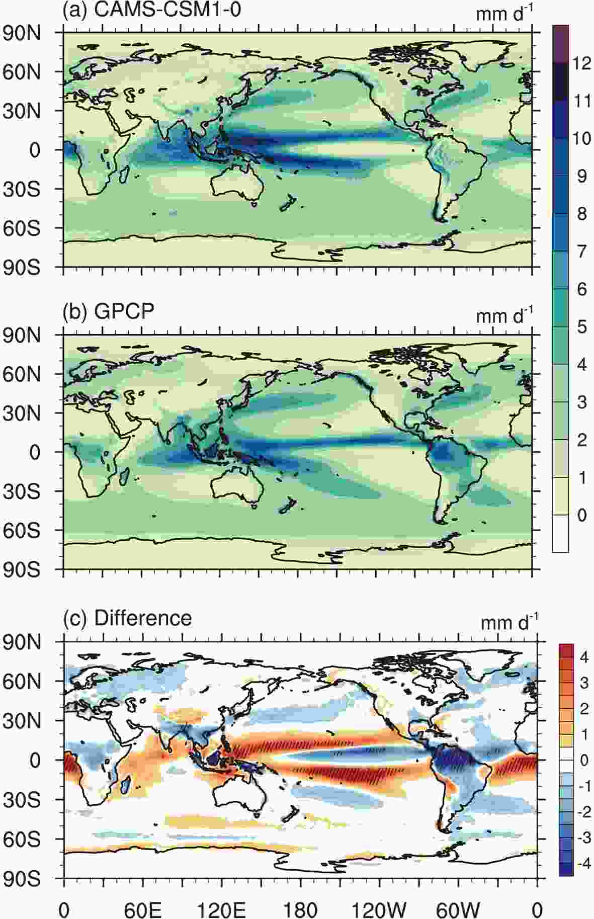 Figure2. The climatology (1980–2014-averaged) of precipitation: (a) ensemble mean of CAMS-CSM historical simulations (r1i1p1f1 and r2i1p1f1); (b) GPCP data; (c) differences between CAMS-CSM historical simulations and GPCP data. The hatched areas in the plots denote the significance level of 5% from the t-test against the interannual anomalies. Units: mm d?1.
The equatorial thermocline plays a crucial role in the climate variability of the tropical Pacific. Fluctuation of the thermocline depth is tightly connected with the sea surface temperature anomalies associated with the ENSO phenomenon. Figure 3 shows the simulated annual mean upper-ocean temperature along the equatorial oceans. Here, we use the depth of the 20°C isotherm to represent the thermocline depth. It can be seen that the west–east-tilted feature of the equatorial Pacific thermocline is well depicted by the model. In the equatorial Pacific, the 20°C isotherm of the model generally follows that of the observation. The discrepancy is that the simulated thermocline exhibits a kind of weaker zonal slope compared with the observation, which is primarily manifested by a slightly shallower thermocline in the model in the western Pacific. The 20°C isotherms in the Indian Ocean and Atlantic Ocean are also reproduced reasonably well, with a weaker slope relative to the observation. Below 150 m in the Pacific Ocean, the isotherms generally follow the observation, while warm biases can be found over the Indian and Atlantic oceans.
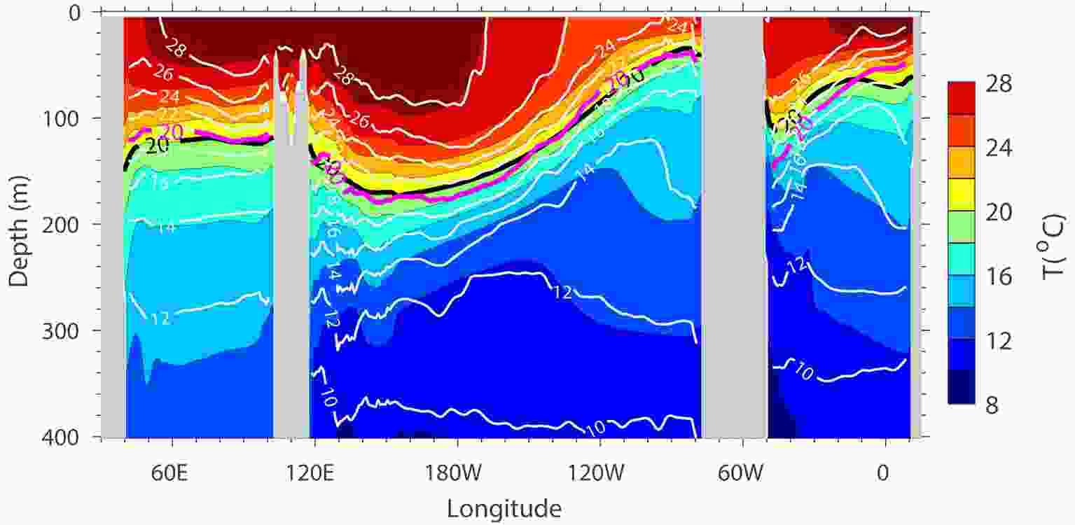 Figure3. Annual mean temperatures (°C) along the equator (5°S–5°N) derived from the CAMS-CSM historical simulation (black contours and shading) and Levitus94 climatology (white contours). The black and red thick lines indicate the 20°C isotherm from CAMS-CSM and the Levitus94 climatology, respectively. units: °C.
Figure 4 shows the climatological mean sea-ice concentration for the historical simulations. The line (thick cyan) of 15% mean concentration from the HadISST data is presented for comparison. In general, the model is able to depict the seasonal evolution of sea-ice concentrations. During February–March–April, the simulated Arctic sea ice extends too much to the equator, in particular over the North Atlantic Ocean, whereas during August–September–October the sea-ice cover is in agreement with the observation. Analogous to the previous version (Rong et al., 2018), the Antarctic sea ice is underestimated by the model, especially during February–March–April, and the sea ice is visible over some areas of the Ross Sea and Weddell Sea. The excessive/insufficient sea-ice cover concentrations in the Arctic/Antarctic leads to the warm/cold biases in the surface temperature over these regions, indicating that the representation of sea ice needs further improvement to enhance the temperature simulation.
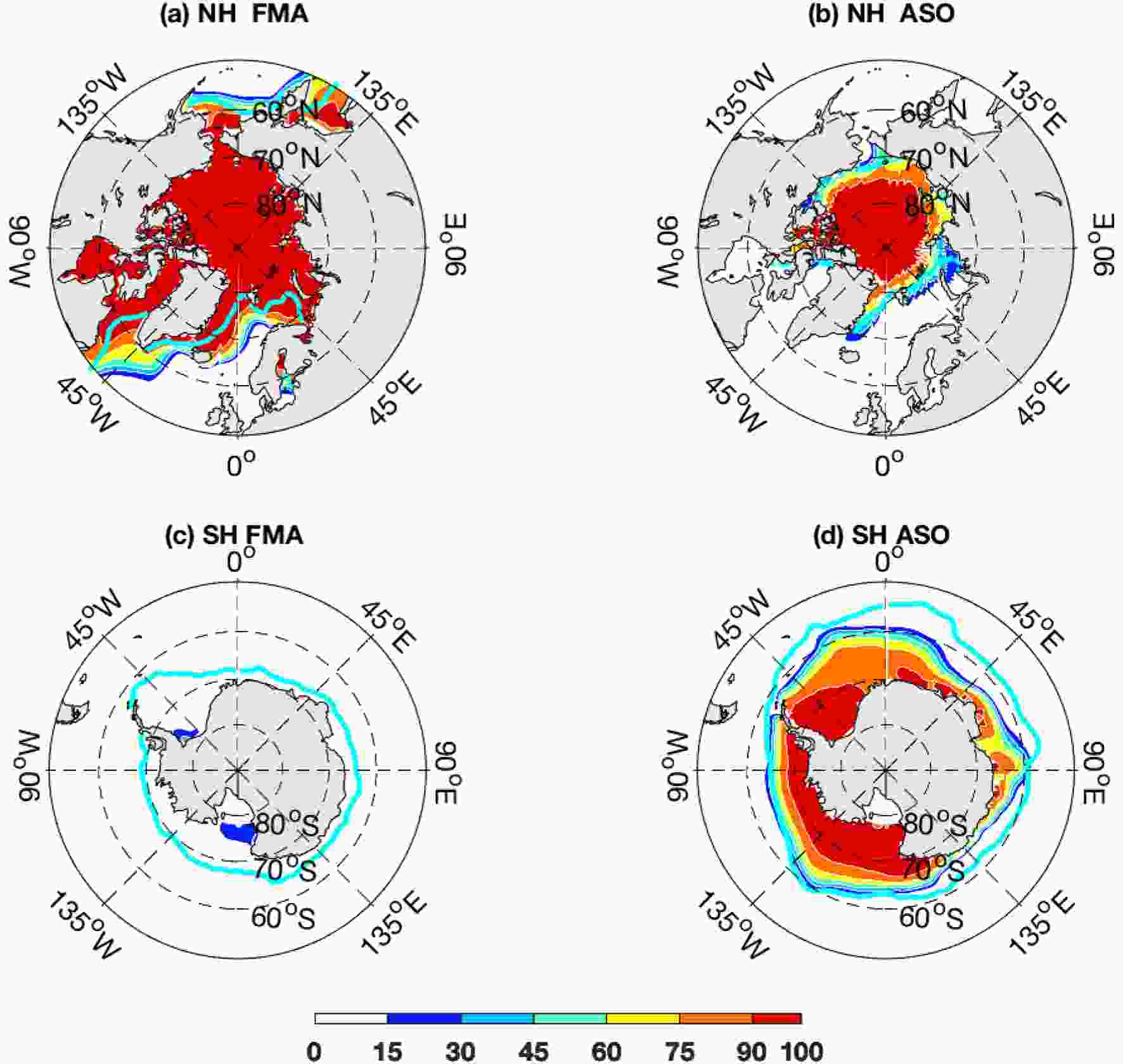 Figure4. Climatological sea-ice concentration in the (a, b) Arctic and (c, d) Antarctic for the period 1980–2014 for the historical simulations. The thick cyan lines indicate the 15% mean concentration values from the HadISST data with the same period. Panels (a, c) and (b, d) denote the averages for February–March–April and August–September–October, respectively. Units: %.
2
4.2. Interannual variability
Figures 5a and b show the standard deviation of the Ni?o3.4 index from the observations and model. It can be seen that the amplitude of the simulated Ni?o3.4 SST variability is closely consistent with the HadISST data. Similar to the observation, the simulated ENSO tends to mature during the winter, indicating a reasonable phase-locking feature produced by the model. In particular, the overestimated ENSO amplitude in the previous version of CAMS-CSM is remarkably reduced, which may be attributable to the improvement in convection and cloud radiative forcing over the tropical Pacific due to the modification of the cumulus scheme. Note that in the current version there is a secondary peak occurring near May, which is not observed in the previous version. The spatial distribution of simulated SST variability also shows a reasonable pattern with respect to the observation (Figs. 5a and b), with the maximum center situated over the central-eastern equatorial Pacific. Compared with the observation, the SST variance is underestimated over the coastal region of South America, which is a common bias in coarse resolution coupled models and can be attributed to the insufficient coastal upwelling in these models.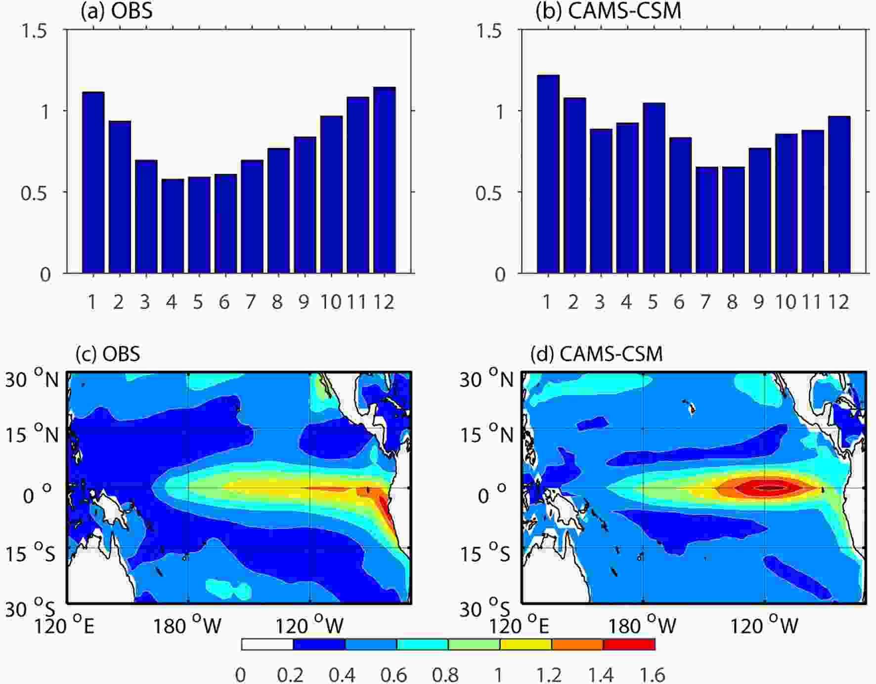 Figure5. Standard deviation of the Ni?o3.4 index [SST anomaly averaged over (5°S–5°N, 170°–120°E)] for each calendar month as derived from the (a) HadISST data and (b) CAMS-CSM. Panels (c, d) show the standard deviation of SST anomalies from HadISST and CAMS-CSM, respectively. Units: °C.
2
4.3. Long-term trend
As mentioned above, the change in global mean surface temperature from pre-industrial times to the present day in the historical simulations is a key metric of the model performance. Figure 6a shows the simulated and observed global mean surface air temperature anomalies from 1850 to 2014. It can be seen that all three ensemble members can reasonably capture the long-term warming trend since 1850, as well as the rapid warming after 1980. As three ensemble members start from different initial conditions or using different forcing, the transient phases among them are inconsistent except during the major volcanic eruption periods. For example, the global mean surface air temperature of “r1i1p1f1” and “r2i1p1f1” shows notable decline near the eruption periods of Krakatoa (1883), Mount Pelée (1902) and Pinatubo (1991), while in “r1i1p1f2” such a global cooling is absent because the stratospheric aerosols are excluded in this simulation. Compared with the observations, the simulated cooling in responses to volcanic eruption is overestimated, especially during Pinatubo’s eruption, leading to a weaker warming in both the “r1i1p1f1” and “r2i1p1f1” experiments after the 1990s. The simulation of “r1i1p1f2”, however, shows a comparable warming trend to that observed. The averaged least-squares linear trends of the three simulations from 1850 to 2014 are 0.041 (r1i1p1f1), 0.040 (r2i1p1f1), and 0.046 (r1i1p1f2) °C (10 yr)?1, which is slightly weaker than that of the observation [0.048°C (10 yr)?1]. Note that the warming of “r1i1p1f2” after 1980 is remarkably stronger than those of “r1i1p1f1” and “r2i1p1f1”. The linear trends of the HadCRUT4 data, “r1i1p1f1”, “r1i1p1f2” and “r1i1p1f2” from 1980 to 2014 are 0.161, 0.137, 0.138 and 0.204°C (10 yr)?1, respectively, suggesting a robust cooling effect of Pinatubo in this model. It can be seen that the warming trend produced in CAMS-CSM is weaker than that of the FGOALS-f3-L, in which the trend tends to be greater than observed, suggesting different climate sensitivities of the two models. The observed precipitation time series exhibits a slight wetting trend after the 1980s, which is captured by the three ensemble members’ simulations. Before the 1980s, the simulated precipitation shows significant interannual fluctuation without an obvious long-term trend.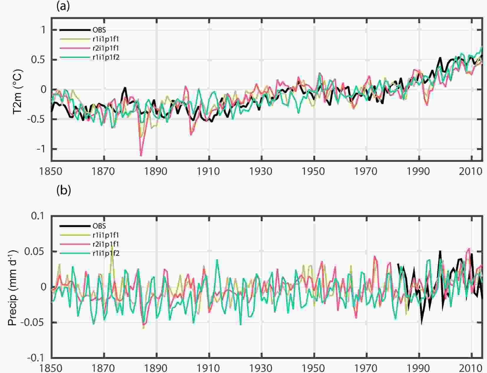 Figure6. Global mean (a) surface air temperature (unit: °C) and (b) precipitation (units: mm d?1) anomalies (annual mean) relative to the period 1961–90 for the CAMS-CSM historical experiments and observation. The observational data for surface air temperature and precipitation are HadCRUT4 and GPCP, respectively.
Figure 7 shows the linear trend of the simulated and observed zonal mean air temperature from 1960 to 2014. In general, the model captures well the major pattern of the trend in air temperature from the surface to 10 hPa. The observed trend of air temperature mainly shows a reversed distribution between the troposphere (below 150 hPa) and stratosphere (above 150 hPa), reflecting a typical structure of air temperature changes in response to increasing GHGs (Fig. 7b). Over the polar region of the Southern Hemisphere, the observed trend exhibits a sandwich structure, i.e., a warming trend below 300 hPa and above 30 hPa, and a cooling trend between 300 hPa and 30 hPa. The model is able to reproduce the reversed trend between the troposphere and stratosphere, and the simulated magnitude of the trend is comparable with that of the observation. Noting that the complex structure over the southern polar region is successfully captured by the model, especially the warming center above 30 hPa, which seems absent in FGOALS-f3-L (Guo et al., 2020), there are nonetheless some deficiencies in the model. For example, the maximum cooling in the model shifts toward to the lower stratosphere, and the warming trend in the lower troposphere over the southern and northern polar regions is somewhat underestimated.
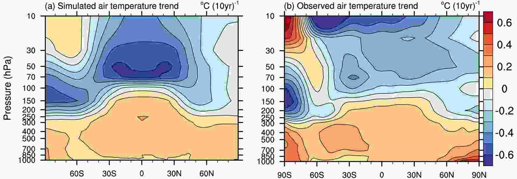 Figure7. Linear trends of zonal mean air temperature from 1960 to 2014 for the (a) ensemble mean of the CAMS-CSM historical experiments (r1i1p1f1 and r2i1p1f1) and (b) observation (JRA-55).
The ocean component (MOM4) and sea-ice component (SIS) of CAMS-CSM use a tripolar grid, which is composed of a bipolar Arctic grid (two northern poles are placed over the North American and Eurasian land areas) and a normal spherical latitude–longitude grid. As the tripolar grid model uses generalized orthogonal curvilinear coordinates, its X and Y directions are orthogonal over the bipolar region, but no longer parallel to latitude–longitude circles. Instead, there are geographically varying angles between two grids. At present, the oceanic and sea-ice output dataset of CAMS-CSM published on the ESGF node are on the original tripolar grid (i.e., the grid label “gn” means the model’s native grid), and thus specific consideration is required before visualization of the datasets. For scalar variables, users can directly analyze and visualize the dataset by software that supports curvilinear grids (i.e., the grids represented by two-dimensional latitude/longitude arrays), such as NCL or Python. An alternative choice is to interpolate the original data to a latitude–longitude grid using CDO or NCO, which can be easily processed by command-line operations. For vector variables over the latitude–longitude grid area (southward of 60°N), users can directly analyze or visualize the data using normal scientific data analysis and visualization software. While over the bipolar Arctic region poleward of 60°N, rotations are needed before visualization or interpolation, which should be performed in terms of the angles between the original orthogonal curvilinear grid and the latitude–longitude grid.
Acknowledgements. This work was supported by the National Key Research and Development Program of China (Grant No. 2019YFC1510001), the National Natural Science Foundation of China (Grant No. 91637210), the Basic Research Fund of CAMS (Grant No. 2018Z007), and the Jiangsu Collaborative Innovation Center for Climate Change.
Open Access This article is distributed under the terms of the Creative Commons Attribution 4.0 International License (
