

中国科学院大学数学科学学院, 北京 100049;中国科学院大数据挖掘和知识管理重点实验室, 北京 100190
摘要: 判断图的连通性质是一个经典的图论问题,也是应用图挖掘和图分解的重要子问题。除了图分解,图的连通性质也被运用于追踪疾病的传播、大型系统设计、社交网络分析和"Cayley图"的一些理论研究。首先综述几种重要的判断无向图是否是连通图的方法,例如广度优先搜索、深度优先搜索和图的拉普拉斯矩阵的特征值。此外,提出一些新方法,例如邻接矩阵的指数和及逻辑和,其中逻辑和是基于搜索方法的计算形式。在随机生成的超过10 000个顶点的图上测试了所有方法,结果显示广度优先搜索和逻辑和方法在超过100个顶点的大图上效果最好,逻辑和最快。
关键词: 连通性广度优先搜索深度优先搜索指数和Laplacian矩阵逻辑和
An undirected graph G=(V, E) consists of a pair of sets: a set of vertices V={v1, v2, …, vN} and a set of edges E={v1, v2, …, vM}, where all the edges are bidirectional. If there are no self-loops, parallel edges, and weights in the undirected graph, it is called a simple graph[1-2], so the "graph" occurred in this paper stands for a simple graph. The graph G is connected if there is a path in G from every vertex to every other vertex[3-4]. When partitioning a graph into several connected components, determining the connectedness of all the components is regarded as a key sub problem. In some previous work, such as Refs.[5-7], connectedness has been ignored, because the objective function aiming at minimizing the total cut makes the connectedness constraint unnecessary. But if we change the objective function, how to determine the connectedness of a graph or part of the graph becomes very important in computing. Apart from graph partitioning, graph connectedness also plays an imperative role in tracking the spread of disease [8], VLSI design [9], social network analysis[10-11], and some theoretical results in graph theory like "Cayley graph" [12].
"How to determine whether a graph is connected or not?" is a frequently asked question on the Internet. Different methods mentioned by people in their blogs or some websites are rarely found or organized in research papers. This paper reviews some main methods for determining the connectedness of a graph, proposes some new ones, and does experiments to compare all the methods.
1 PreliminariesThere are several different ways to represent a graph G=(V, E), among which adjacency matrix is the most widely used and if the adjacency matrix is given, the graph is fixed correspondingly. Adjacency matrix A={ai, j}N×N shows the connection between vertex and vertex [2], where vi, vj∈V, N is the number of vertices and
| ${a_{i, j}} = \left\{ \begin{gathered} 1, \;\;\;{\text{if}}\;\;{v_i}\;{\text{and}}\;{v_j}\;{\text{are}}\;{\text{connected}}{\text{.}} \hfill \\ {\text{0, }}\;\;\;{\text{otherwise}}{\text{.}} \hfill \\ \end{gathered} \right.$ |
Another important concept used in this paper is Laplacian matrix, which is also a popular matrix representation of a graph. Given a graph G on N vertices, its Laplacian matrix is the n-by-n matrix L(G)=D(G)-A(G), where A(G) is the adjacency matrix, and D(G) is the degree matrix.
For example, given a graph G=(V, E) with V={u, v, w, x, y} and E={uv, uw, vw, vx, wx, xy}. The adjacancy matrix A of the graph G is
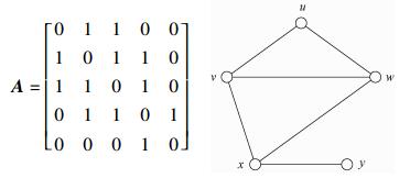 |
| $\mathit{\boldsymbol{L}} = \mathit{\boldsymbol{D}}- \mathit{\boldsymbol{A}} = \left[{\begin{array}{*{20}{l}} 2&{-1}&{-1}&0&0 \\ {-1}&3&{ - 1}&{ - 1}&0 \\ { - 1}&{ - 1}&3&{ - 1}&0 \\ 0&{ - 1}&{ - 1}&3&{ - 1} \\ 0&0&0&{ - 1}&1 \end{array}} \right]$ |
Last but not least, the "distance" between two vertices in a graph is the number of edges in a shortest path connecting them.
2 MethodsThere are three different types of methods for determining the connectedness of a graph:
1) Search methods, including breadth-first search, depth-first search, random walks methods.
2) Algebraic computation on adjacency matrix or Laplacian matrix of the graph, such as power, eigenvalue, and logical sum.
3) Path finding: shortest path algorithms like Dijkstra, Warshall, Floyd algorithm.
In order to determine the connectedness of a graph by path finding methods, the paths between one vertex and all the other vertices should be found, which is very time consuming and complicated. So we combine the second with third methods and apply the path finding methods on the computation of adjacency matrix.
2.1 Search methods2.1.1 Breadth-first searchBreadth-first search was first proposed by Ref.[13] in 1950s to find the shortest path out of a maze, and invented independently by Ref.[14] for solving efficiently path-connection problems.
Making use of breadth-first search to determine the connectedness of a graph can be interpreted as three steps:
1) Put one chosen vertex into the waiting list (shorten as "WL") and mark it;
2) Move the first vertex WL1 in WL to SL (short for "search list") and put all the unmarked vertices within the distance of 1 with WL1 into WL from the back and mark them.
3) Repeat second step until there is no vertex in WL. If the elements in SL are all the vertices of the graph, the graph is connected.
Figure 1 shows an example of the procedure to do breadth-first search on a graph.
Fig. 1
 | Download: JPG larger image |
Fig. 1 Breadth-first search | |
The time complexity of breadth-first search algorithm is O(|V|+|E|), where V is the number of vertices and E is the number of edges, because the worst case is that all the edges and vertices are visited[15].
2.1.2 Depth-first searchDepth-first search was investigated in the 19th century for the use of solving mazes[16].
Determining the connectedness of a graph by the use of depth-first search algorithm works in the following three steps:
1) Pick up a starting vertex to SL and mark it; FL (formal list)=[0];
2) Put one unmarked vertex directly connected with the last vertex in SL into SL and mark it. Record the formal chosen vertex of the newly chosen vertex in FL.
3) Repeat second step until there is no unmarked vertex connected to the chosen vertex, and roll back to the formal chosen vertex by the use of FL. Stop until search back to 0 in the FL. If the elements in SL are all the vertices, the graph is connected.
Figure 2 shows an example of the procedure to do depth-first search on a graph. The time complexity of this algorithm is Θ(|V|+|E|)[15] which is similar with the breadth-first search, so the choice of these two algorithms depends on different situations and their different properties instead of their time complexities.
Fig. 2
 | Download: JPG larger image |
Fig. 2 Depth-first search | |
2.1.3 Random walks algorithmRandom walks, first propose in 1905[17], have been widely used in many fields: physics, computer science, chemistry, and so on[18-19]. A random walk is a path that consists of a series of random behaviors or steps.The algorithm can not stop until all the vertices are visited or the number of steps exceeds a given integer. The algorithm is shown in Algorithm 1.
| Algorithm 1 Random walks algorithm |
| Require: rand: Random number; A: Adjacency matrix; K: An integer, SL: visiting list |
| Ensure:SL |
| 1:Initial next←v, i←0 |
| 2:Generate rand, and i←i+1. The degree of vertex next is deg(next). |
| 3: |
| 4:next←vi |
| 5:end if |
| 6:Repeat step 2 to step 5, and stop when all the vertices are visited or i>K. |
| 7:Output: SL |
| $\mathit{\boldsymbol{P}} = \mathit{\boldsymbol{I}} + \mathit{\boldsymbol{A}} + {\mathit{\boldsymbol{A}}^2} + {\mathit{\boldsymbol{A}}^3} + \cdots + {\mathit{\boldsymbol{A}}^{N-1}}, $ | (1) |
If all the elements in the first row of P are larger than 0, the graph G is connected. The idea of power sum method is similar with Warshall algorithm, aiming at finding all the shortest paths between a certain vertex and all the other vertices. The computation complexity of power sum method is O(N3).
2.2.2 Laplacian matrixLaplacian matrix is another important matrix representation of a graph and have been used to calculate a lot of important properties of the graph[21]. There are many characteristics of the eigenvalues of graph Laplacian matrix, among which the theory: the number of connected components of G is equal to the multiplicity of 0 as an eigenvalue[22] can be used to determine the connectedness of a graph. In general, the time complexity of this method is O(N2)[23].
2.2.3 Logical sum of adjacency matrixThis method is the computational version of search methods. Logical sum is a basic computation in computer science and also similar with the definition of "union" and "or". As we know, if a vertex i isconnected with j, j is connected with m, and then i is connected with m. It is the same idea with the logical sum:
0+0=0, 0+1=1+0=1+1=1.
Applying logical sum to graph computation was firstly proposed in a Spanish book in 1992. We propose one new method with two different versions based on logical sum. The implementation of logical sum on determining the connectedness of a graph is summarized in Algorithm 2.
| Algorithm 2 Logical sum algorithm (version 1) |
| Require A: Adjacency matrix, V={V1, V2, …, VN}, V1 is marked. |
| 1:Pick up one vertex Vj, where |
| 2:Renew the value of the first row by the logical sum of the first row and the jth row; replace all the elements in column j and row j with 0. |
| 3:Repeat step 1 and 2 until there is no "1" left in the first row. If all the vertices are marked, the graph is connected. |
| Algorithm 3 Logical sum algorithm (version 2) |
| Require A: Adjacency matrix, V={V1, V2, …, VN}, V1 is marked. |
| 1:Pick up all the vertices M={Vj}, where arg{a1, j=1} and mark them. Note: arg{a1, j=1} means all the js which meet a1, j=1. |
| 2:Renew the value of the first row by the logical sum of the first row and all the rows in M; replace all the elements in columns M and rows M with 0. |
| 3:Repeat step 1 and 2 until there is no "1" left in the first row. If all the vertices are marked, the graph is connected. |
3 Numerical experimentsSince the time complexity of random walk method is unknown and we want to show that logical sum method shows better than other methods in real experiments because of its computational idea. We conducted numerical experiments to compare all the methods mentioned in the third section. (DS: depth-first sesarch; BS: breadth-first search; RW: random walk; PS: power sum; LM: Laplacian matrix; LS (1): logical sum (1); LS (2): logical sum (2))
Table 1 to Table 5 and Fig. 3 present the results.
Table 1
| Table 1 Numerical experiments on graphswith 10 vertices | ||||||||||||||||||||||||||||||||||||||||||||||||
Table 2
| Table 2 Numerical experiments on graphs with 100 vertices | ||||||||||||||||||||||||||||||||||||||||||||||||
Table 3
| Table 3 Numerical experiments on graphs with 1 000 vertices | ||||||||||||||||||||||||||||||||||||||||||||||||
Table 4
| Table 4 Numerical experiments on graphs with 10 000 vertices | ||||||||||||||||||||||||||||||||||||||||||||||||
Table 5
| Table 5 Numerical experiments on graphs with 20 000 and 30 000 vertices | ||||||||||||||||||||
In order to show their performance on different scale of graphs, four sets of experiments on random graphs with up to 10 000 vertices have been done. After that, well performed methods: breadth-first search and logical sum are applied to random graphs with 20 000 and 30 000 vertices.
In the four sets of experiments, each method was run third times on random graphs with 10, 100, 1 000, and 10 000 vertices, respectively.
In the fifth set of experiments, breadth-first search and logical sum are applied to random graphs with 20 000 and 30 000 vertices.
4 Main resultsIn our first to fourth set of experiments, each method is applied three times on random graphs and the random graph in every round is the same. Power sum takes the least time when there is only 10 vertices in a graph and breadth-first search follows. While in the second set of experiments, breadth-first search method is the fastest algorithm, and power sum follows. When there is more than 1 000 vertices in the graph, the advantage of logical sum algorithm becomes more and more obvious. Besides, random walk method is not stable since the way of producing next chosen vertex is not stable. Figure 3 shows the running time of different methods changing over the number of vertices in the graph.
Fig. 3
 | Download: JPG larger image |
Fig. 3 Performances of different methods | |
As shown in Table 5, breadth-first search and logical sum are very fast when dealing with large graphs and logical sum (version 2) is the best which saves almost half of the running time of breadth-first search.
5 ConclusionDepth-first search and breadth-first search are well-known and widely used methods. They are very easy and fast, but breadth-first search are much faster in determining the connectedness of a graph than depth-first search method and breadth-first search method is also very competitive in comparison with algebraic methods. Another search method: random walks method is easily developed, but not very stable in application.
Power sum method is always faster than the Laplacian matrix method and it is also faster than logical sum methods when the graph is small. However, when the number of vertices of a graph grows, logical sum methods are more efficient.
Since there are a lot of packages and tools for those old methods, if the graph is not so complicated and large, the breadth-first search is the best choice. But if the graph is very large, loogical sum (version 2) method is very easy to develop and extremely fast, which should be a very good choice.
References
| [1] | Alan G. Algorithmic graph theory[J]. Oberwolfach Reports, 1989, 3(1): 379-460. |
| [2] | Douglas B W. Introduction to graph theory[M]. 2nd ed. Upper Saddle River: Prentice hall, 2001. |
| [3] | Robert S, Kevin W. Algorithms[M]. 4th ed. Boston: Addison-Wesley Professional, 2011. |
| [4] | Santanu S R. Graph theory with algorithms and its applications:in applied science and technology[M]. India: Springer, 2013. |
| [5] | Lorenzo B, Michele C, Giovanni R. A Branch-and-cut algorithm for the Equicut problem[J]. Mathematical Programming, 1997, 78(2): 243-263. DOI:10.1007/BF02614373 |
| [6] | John E M. Branch and cut for the k-way Equipartition Problem[J]. Discrete Optimization, 2007, 4(1): 87-102. DOI:10.1016/j.disopt.2006.10.009 |
| [7] | Stefan E K, Franz R, Jens C. Solving graph Bisection problems with Semidefinite Programming[J]. INFORMS Journal on Computing, 2000, 12(3): 177-191. DOI:10.1287/ijoc.12.3.177.12637 |
| [8] | Huang A, Zhu W. Connectedness of graphs and its application to connected matroids through covering-based rough sets[J]. Soft Computing, 2016, 20(5): 1841-1851. DOI:10.1007/s00500-015-1859-2 |
| [9] | Andrew B K, Jens L, Igor L M, et al. VLSI physical design:from Born graph partitioning to timing closure[M]. Hamburg: Springer, 2011. |
| [10] | Maria C, Bernard R, Yori Z. Claw-free graphs with strongly perfect complements:fractional and integral version. part Ⅰ. Basic graphs[J]. Discrete Applied Mathematics, 2011, 159(17): 1971-1995. DOI:10.1016/j.dam.2011.06.024 |
| [11] | James A B. Graph theory and social networks:a technical comment on connectedness and connectivity[J]. Sociology, 1969, 3(2): 215-232. DOI:10.1177/003803856900300205 |
| [12] | Laszlo B. Some applications of graph contractions[J]. Journal of Graph Theory, 1977, 1(2): 125-130. DOI:10.1002/(ISSN)1097-0118 |
| [13] | Edward F M. The shortest path through a maze[J]. In proceedings of the International Symposium on the Theory of Switching, 1959, 285-292. |
| [14] | Lee C Y. An algorithm for path connections and its applications[J]. IRE Transactions on Electronic Computers, 1961, 3(1): 346-365. |
| [15] | Thomas H C, Charles E L, Ronald L R, et al. Introduction to algorithms[M]. 3rd edition. Cambridge: MIT Press, 2001. |
| [16] | Shimon E. Graph algorithms[M]. Cambridge and New York: Cambridge University Press, 2011. |
| [17] | Pearson K. The problem of the random walk[J]. Nature, 1905, 72(1865): 294. |
| [18] | Kampen N G. Stochastic processes in physics and chemistry[M]. Revised and enlarged edition. Amsterdam/London/New York/Tokyo: Elsevier, 1992. |
| [19] | Pierre D G. Scaling concepts in polymer physics[M]. Ithaca and London: Cornell University Press, 1979. |
| [20] | Sriram V P, Steven S S. Computational discrete mathematics:combinatorics and graph theory with mathematica[M]. Cambridge: Cambridge University Press, 2009. |
| [21] | Chung F. Spectral graph theory[M]. New York: American Mathematical Society, 1997. |
| [22] | Michael W N. The Laplacian spectrum of graphs[D]. Manitoba: University of Manitoba, 2000. |
| [23] | Li T Y. The Laguerre tteration in solving the symmetric tridiagonal eigenproblem, revisited[J]. SIAM Journal on Scientific Computing, 1994, 15(5): 1145-1173. DOI:10.1137/0915071 |
