 ,1,2
,1,2Molecular clock dating using MrBayes
ZHANG Chi,1,2通讯作者: zhangchi@ivpp.ac.cn
收稿日期:2019-01-14网络出版日期:2019-07-20
| 基金资助: |
Corresponding authors: zhangchi@ivpp.ac.cn
Received:2019-01-14Online:2019-07-20

摘要
介绍了利用MrBayes进行分子钟定年的研究概况和程序。利用一个整合分子序列和形态特征的膜翅目昆虫的数据,展示了两种现代方法:全证据定年和节点定年,并对这两种方法的相似点和不同之处进行比较和讨论。此外,还用无分子钟的方法对同一数据进行分析,并与分子钟定年法进行比较。
关键词:
Abstract
This paper provides an overview and a protocol of molecular clock dating using MrBayes. Two modern approaches, total-evidence dating and node dating, are demonstrated using a truncated dataset of Hymenoptera with molecular sequences and morphological characters. The similarity and difference of the two methods are compared and discussed. Besides, a non-clock analysis is performed on the same dataset to compare with the molecular clock dating analyses.
Keywords:
PDF (1523KB)元数据多维度评价相关文章导出EndNote|Ris|Bibtex收藏本文
本文引用格式
张驰. MrBayes分子钟定年之程序. 古脊椎动物学报[J], 2019, 57(3): 241-252 DOI:10.19615/j.cnki.1000-3118.190408
ZHANG Chi.
1 Introduction
MrBayes is a software for Bayesian phylogenetic inference (Huelsenbeck and Ronquist, 2001; Ronquist and Huelsenbeck, 2003) and has become widely used by biologists (Van Noorden et al., 2014). Many new features have been implemented since version 3.2 (Ronquist et al., 2012b), including species tree inference under the multi-species coalescent model (Liu, 2008; Liu et al., 2009); compound Dirichlet priors for branch lengths (Rannala et al., 2012; Zhang et al., 2012); marginal model likelihood estimation using stepping-stone sampling (Xie et al., 2011); topology convergence diagnostics using the average standard deviation of split frequencies (Lakner et al., 2008); BEAGLE library support (Ayres et al., 2012) and parallel computing using MPI (Altekar et al., 2004).In addition to these features, the focus of this study is its new functionality of divergence time estimation using node dating (Yang and Rannala, 2006; Ho and Phillips, 2009) and total-evidence dating (Ronquist et al., 2012a; Zhang et al., 2016) approaches under relaxed molecular clock models (Huelsenbeck et al., 2000; Thorne and Kishino, 2002; Drummond et al., 2006; Lepage et al., 2007). Both dating techniques are implemented in the Bayesian framework, such that the diversification process and the fossil information are incorporated in the priors. However, they do have significant differences. In node dating, only molecular sequences from extant taxa are used, and one or more internal nodes of the extant taxon tree are calibrated by user-specified prior distributions, typically derived from the fossil record, to estimate the ages of all other nodes in the tree. In total-evidence dating, extant and extinct taxa are all included in the tree, and morphological characters are coded for fossil and extant taxa in a combined matrix with molecular sequences. The age of each fossil is assigned a prior distribution directly.
Several steps are involved in a Bayesian molecular clock dating analysis, importantly including partitioning the data, specifying evolutionary models, calibrating internal nodes or fossils, and setting priors for the tree and the other parameters. In this paper, I introduce a general clock dating protocol that could potentially be applied to a wide range of taxonomic groups, using a truncated Hymenoptera data as an example.
The original data analyzed by Ronquist et al. (2012a) and Zhang et al. (2016) includes 60 extant and 45 fossil Hymenoptera (wasps, ants, and bees) and eight outgroup taxa. The data were divided into eight partitions as follows: 1) morphology, 2) 12S and 16S, 3) 18S, 4) 28S, 5) 1st and 2nd codon positions of CO1, 6) 3rd codon positions of CO1 (but not used in the analyses), 7) 1st and 2nd codon positions of both copies of EF1α, and 8) 3rd codon positions of both copies of EF1α. These are based on morphological characters, mitochondrial and nuclear genes. The full data takes days to run. For illustrative purposes, the data is truncated into ten extant taxa (nine Hymenoptera and one Raphidioptera) and ten fossils, with 200 morphological characters, 100 sites from 16S, and 210 sites from EF1α. Below, the dataset is analyzed by both total-evidence dating and node dating approaches under diversified sampling of extant taxa (H?hna et al., 2011; Zhang et al., 2016), followed by a non-clock analysis under the compound Drichlet prior for branch lengths (Rannala et al., 2012; Zhang et al., 2012).
2 Protocol
2.1 MrBayes installation
The program MrBayes is available from GitHub (https://github.com/NBISweden/MrBayes), including pre-compiled executables for macOS and Windows, and source code for all platforms. The current version is 3.2.7, which is used here. The truncated dataset hym.nex is in the doc/tutorial folder within the release. For convenience, it is recommended to put it in the same directory as the executable (e.g., named mb in macOS/Linux or mb.exe in Windows). The file hym.nex in the NEXUS format can be opened by a text editor or a matrix editor such as Mesquite (https://www.mesquiteproject.org). The data matrix is at the beginning, including morphological characters and molecular sequences. Following the data block, users can write MrBayes commands within the mrbayes block (each ends with a semicolon). These commands will be executed automatically when the data is read in. The texts within a pair of square brackets are comments and will be ignored by the program.In terminal (macOS/Linux) or command prompt (Windows), navigate to the folder containing the executable and data file using the cd command, and launch MrBayes using ./mb (macOS/Linux) or mb.exe (Windows). The following header will appear.
MrBayes 3.2.7 x86_64
(Bayesian Analysis of Phylogeny)
Distributed under the GNU General Public License
MrBayes >
The prompt at the bottom means that MrBayes is running and ready for your commands. Simply use
execute hym.nex
to read in the data.
2.2 Data partitions
When the data is read in, the commands for defining the partitions are also executed.charset MV = 1-200
charset 16S = 201-300
charset Ef1a = 301-510
charset Ef1a12 = 301-510\3 302-510\3
charset Ef1a3 = 303-510\3
partition four = 4: MV, 16S, Ef1a12, Ef1a3
set partition = four
Here we define four partitions: the morphology (MV), 16S, 1st and 2nd codon positions of EF1α (Ef1a12), and 3rd codon positions of EF1α (Ef1a3). The name “four” is user defined and can be any other string. Note the semicolon (;) at the end of each command is neglected as the command is supposed to be typed after the MrBayes prompt (a semicolon is necessary when the command is written in a file, the same below).
2.3 Substitution models
For the morphological partition, the Mkv model (Lewis, 2001) is used with variable ascertainment bias (only variable characters scored), equal state frequencies and gamma rate variation across characters.lset applyto = (1) coding = variable rates = gamma
Constant characters will be excluded automatically by the program. To be specific, use the following command to exclude them.
exclude 7 31 61 83 107 121 122 133 182 183 198
If instantaneous change is only allowed between adjacent states (e.g., 0?1 and 1?2 but not 0?2), these characters are specified using this command.
ctype ordered: 20 23 27 30 36 41 42 44 46 48 59 65 75 78 79 89 99 112 117 134 146 157 159 171 185 191 193 196
The other characters are thus unordered which can change instantaneously from one state to another. Dollo or irreversible character is not supported in MrBayes at the moment.
For the molecular partitions, the general time-reversible model is used with gamma rate variation across sites (GTR+Γ) (Yang, 1994a,b).
lset applyto = (2,3,4) nst = 6 rates = gamma
The prior for the gamma shape parameter is exponential(1.0), which can be changed using prset shapepr. We keep the default here.
Different partitions are assumed to have independent substitution parameters, thus we unlink them. The partition-specific rate multipliers are used to account for rate variation across partitions with average to 1.0.
unlink statefreq = (all) revmat = (all) shape = (all)
prset applyto = (all) ratepr = variable
2.4 Relaxed clock models
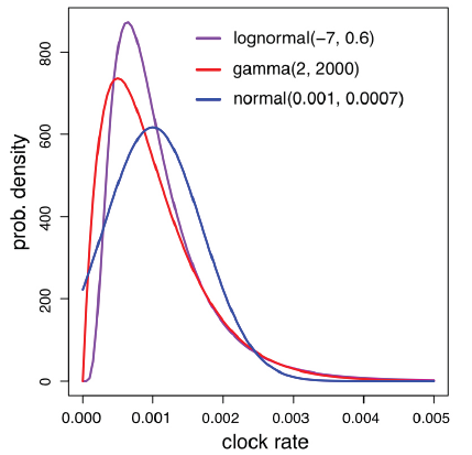
The relaxed clock models account for evolutionary rate variation over time and among branches, and it is now a standard practice to accommodate such variation in dating analyses. There are three relaxed clock models implemented in MrBayes: compound Poisson process (CPP; Huelsenbeck et al., 2000), autocorrelated lognormal (TK02; Thorne and Kishino, 2002) and independent gamma rate (IGR; Lepage et al., 2007). However, the CPP model is computationally not compatible with total-evidence dating, thus we only focus on the IGR and TK02 models. The outcomes of using these two models are discussed below.The mean clock rate (mean substitution rate per site per Myr) is assigned a lognormal(-7, 0.6) prior, with mean 0.001 and standard deviation 0.0007.
prset clockratepr = lognorm(-7,0.6)
The prior is chosen by comparing the age of the oldest insect fossil with the root age estimation from uncalibrated clock analysis as discussed in Ronquist et al. (2012a). One might need to specify a different suitable distribution. There are several options for the clock rate prior, including fixed, normal (truncated at zero), lognormal, and gamma. The probability density functions (all with mean 0.001 and standard deviation 0.0007) are shown in Fig. 1. The differences in this case are minor.
Fig. 1
 新窗口打开|下载原图ZIP|生成PPT
Fig. 1Probability density functions of lognormal, gamma, and normal distributions, all with mean 0.001and standard deviation 0.0007
The relative clock rates, which are mul-tiplied by the mean clock rate, vary differently along the branches of the tree in different models. The TK02 model assumes that the relative rate changes along the branches as Brownian motion on the log scale, starting from 1.0 (0.0 on the log scale) at the root. The rate at the end of a branch is lognormally distributed with mean equal to the rate at the beginning of the branch. Thus the rates at different branches are autocorrelated.
prset clockvarpr = tk02
prset tk02varpr = exp(1)
The IGR model assumes that the relative rate at each branch is an independent gamma distribution with mean 1.0. The variance is proportional to the branch length. Thus the rates are independent of each other (but not identically distributed).
prset clockvarpr = igr
prset igrvarpr = exp(10)
Note that when the relative rates are all fixed to 1.0 in the TK02 or IGR model, it becomes the strict clock model.
Before the total-evidence dating and node dating analyses, we first define the fossil taxa and some constraints for later use. Note these constraints are not enforced until we set topologypr explicitly (see below).
taxset fossils = Asioxyela Nigrimonticola Xyelotoma Undatoma Dahuratoma Cleistogaster Ghilarella Mesorussus Prosyntexis Pseudoxyelocerus
constraint HymenFossil = 2-.
constraint Hymenoptera = 2-10
constraint Holometabola = 1-10
constraint Tenthredinidae = 3-5
constraint CepSirOruApo = 7-10
The numbers here refer to the taxon numbers ordered as in the data matrix, while a dot (.) means the last taxon.
2.5 Total-evidence dating
In the following, we assign priors for the fossils from the geological times. This is a typical step in total-evidence dating, where we calibrate the fossil taxa instead of the internal nodes of the tree. Fossil age uncertainties are represented as uniform distributions, while fixed values can be used when the geological age is very certain.calibrate
Asioxyela = unif(228,242)
Nigrimonticola = unif(152,163)
Xyelotoma = unif(152,163)
Undatoma = unif(145,152)
Dahuratoma = fixed(134)
Cleistogaster = unif(168,191)
Ghilarella = unif(113,125)
Mesorussus = unif(94,100)
Prosyntexis = unif(80,86)
Pseudoxyelocerus = fixed(182)
prset nodeagepr = calibrated
To enable the calibrations, the last nodeagepr command must be present.
The speciation, extinction, fossilization, and sampling process is explicitly modeled using the fossilized birth-death (FBD) process (Stadler, 2010; Heath et al., 2014; Gavryushkina et al., 2014; Zhang et al., 2016).
prset brlenspr = clock:fossilization
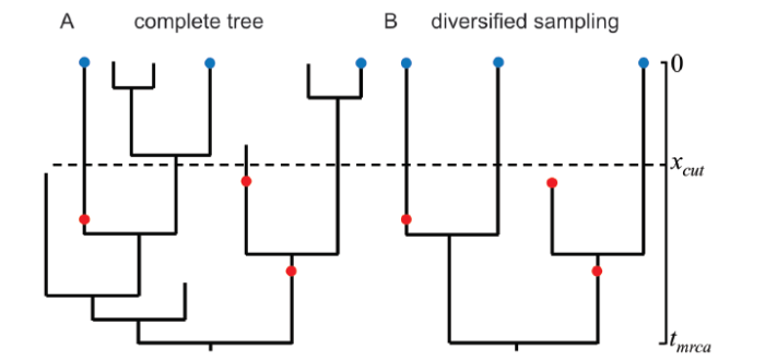
Diversified sampling (Zhang et al., 2016) is arguably suitable for such higher-level taxa, which assumes exactly one representative extant taxa per clade descending from time xcut is sampled, and the fossils are sampled with a non-zero rate before xcut and zero after. A fossil can be either a tip or a sampled ancestor (Fig. 2).
Fig. 2
 新窗口打开|下载原图ZIP|生成PPT
Fig. 2The fossilized birth-death (FBD) process and diversified sampling of extant taxa Exactly one representative taxa per clade descending from time xcut is sampled (blue dots). The fossils are sampled with a constant rate between tmrca and xcut (red dots)
prset samplestrat = diversity
By default, the sampling strategy for extant taxa is uniformly at random (samplestrat = random) which is not used here, but see Zhang et al. (2016) for the application.
The model has four parameters: speciation rate λ, extinction rate μ, fossil discover rate ψ, and extant sample proportion ρ. For inference, we re-parametrize the parameters as d = λ - μ, r = μ / λ, and s = ψ / (μ + ψ), so that the latter two parameters range from 0 to 1. ρ is fixed to 0.0001, based on the living number of Hymenoptera at about 100000 (10/100000 = 0.0001).
prset sampleprob = 0.0001
prset speciationpr = exp(10)
prset extinctionpr = beta(1,1)
prset fossilizationpr = beta(1,1)
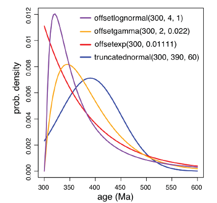
prset treeagepr = offsetexp(300,390)
The FBD prior is conditioned on the root age (tmrca). Here we use an offset exponential distribution with minimal age 300 Ma (according to the oldest neopteran fossil) and mean age 390 Ma (the oldest insect fossil). Users should specify a reasonable root age prior according to the available fossil information. Several available probability densities all with mean 390 and minimal 300 are shown in Fig. 3. The exponential prior is more diffused than the rest three.
Fig. 3
 新窗口打开|下载原图ZIP|生成PPT
Fig. 3Probability density functions of offset lognormal, offset gamma, offset exponential,and truncated normal distributions, all with mean 390 and minimum 300
An alternative tree prior that can be used in the total-evidence dating approach is the uniform prior (clock:uniform) (Ronquist et al., 2012a). It assumes that the internal nodes are draw from uniform distributions and the fossils are only tips of the tree (so-called tip dating). Similarly to the FBD prior, the uniform prior is also conditioned on the root age and requires setting treeagepr.
In order to root the tree properly, we enforce the constraint HymenFossil defined above. This forces the Hymenoptera with fossils to form a monophyletic group.
prset topologypr = constraint(HymenFossil)
For the Markov chain Monte Carlo (MCMC) (Metropolis et al., 1953; Hastings, 1970), we use two independent runs and four chains (one cold and three hot) per run for 500000 iterations and sample every 100 iterations.
mcmcp nrun = 2 nchain = 4 ngen = 500000 samplefr = 100
mcmcp filename = hym.te printfr = 1000 diagnfr = 5000
mcmc
The output file names all start with hym.te (represented as hym.te.*). The chain states are printed to screen every 1000 iterations, and the convergence diagnostics are printed every 5000 iterations. The mcmc command executes the MCMC run.
While the MCMC is running, the iteration number, likelihood values, and average standard deviation of split frequencies (ASDSF) are printed to the screen. The ASDSF should be decreasing toward 0, indicating the tree topologies sampled from the two different runs are getting similar and converging to the same (stationary) distribution. Typically, ASDSF < 0.01 is a good sign of consistency between runs.
To summarize the parameters and trees after the MCMC, use
sump
sumt
By default, the first 25% samples are discarded as burnin. This can be adjusted according to the likelihood traces from the two runs (e.g. viewed in Tracer). The effective sample size (ESS) is an important indicator to judge if sufficient MCMC samples are collected. Ideally, the ESS should be larger than 100 for all parameters. We may need to increase the chain length and adjust MCMC proposals to improve the estimates.
The consensus tree including all fossils is highly unresolved due to the uncertainty in the placement of the fossils. In order to display the node ages clearly, we can redraw an extant taxa tree by pruning the fossils. The output filename is changed to avoid overwriting the existing ones.
delete fossils
sumt output = hym.rf
Note here this sumt command does not rerun the MCMC but just for displaying the extant taxon tree.
2.6 Node dating
In node dating, we calibrate the internal nodes of the tree instead of the fossils above. The morphological characters of the fossils are not used, thus we remove them.delete fossils
exclude 24 130 168
calibrate
Tenthredinidae = offsetgamma(100,150,25)
CepSirOruApo = truncatednormal(140,175,25)
prset nodeagepr = calibrated
The birth-death prior under diversified sampling (H?hna et al., 2011) is used for the time tree. Compared to the FBD prior used above, there is no fossil sampling parameter in this case. The priors for the root age, speciation and extinction rates are not changed.
prset brlenspr = clock:birthdeath
prset samplestrat = diversity
prset sampleprob = 0.0001
prset speciationpr = exp(10)
prset extinctionpr = beta(1,1)
prset treeagepr = offsetexp(300,390)
The uniform tree prior (clock:uniform) is also applicable.
It is important to force the calibrated clade to be monophyletic and enable the constraints. The constraint Hymenoptera helps to root the tree properly.
prset topologypr = constraint(Hymenoptera, Tenthredinidae, CepSirOruApo)
The output filename is changed to avoid overwriting the existing ones. If the node dating analysis is continued after the total-evidence dating in the same MrBayes session, the starting values also need to be reset. The other settings are kept the same as in the total-evidence dating analysis.
mcmcp filename = hym.nd startp = reset startt = random
2.7 Non-clock analysis
Lastly, we run an analysis without the molecular clock assumption and calibrations. The branch lengths are measured by genetic distance (expected substitutions per site). This is a typical analysis most people do using MrBayes. We do not use fossils, and do not constrain the topology so that they are uniformly distributed.delete fossils
prset brlenspr = uncons:gammadir(1,1,1,1)
prset topologypr = uniform
mcmc filename = hym.un
sump
sumt
The prior for branch lengths is gamma-Dirichlet(1, 1, 1, 1) (Rannala et al., 2012; Zhang et al., 2012), which assigns gamma(1, 1) for the tree length and uniform Dirichlet for the proportion of branch lengths. The compound Dirichlet prior was shown to help avoid overestimating the tree length (Zhang et al., 2012) and is now the default prior in MrBayes (since 3.2.3).
3 Results and discussion
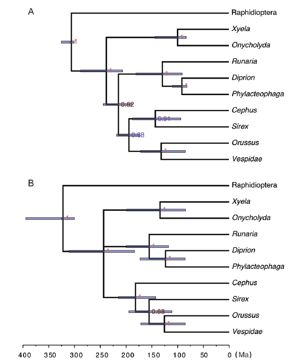
The posterior estimates of the parameters are summarized in separate files, which can be opened using a text editor. The information is also printed to the screen. The partition rate multipliers are in hym.*.pstat (here * is to match te and nd, the same below). The morphologies (m{1}) and 16S (m{2}) partitions evolve at similar rate. The 1st and 2nd codon positions of Ef1α (m{3}) evolve much more slowly than the 3rd codon position (m{4}). Thus it is reasonable to take into account such significant rate variation across partitions.The majority-rule consensus trees are summarized in hym.*.con.tre, which can be visualized by FigTree (http://tree.bio.ed.ac.uk/software/figtree) or IcyTree (https://icytree.org). The node ages are also in hym.*.vstat, associated with the bipartition IDs in hym.*.parts. The root ID is 0 which includes all taxa, while the ID of Hymenoptera is that which excludes the outgroup Raphidioptera (.*********). The extant taxa trees from total-evidence dating and node dating under diversified sampling and IGR clock model are shown in Fig. 4. The topologies are the same in general, except for the Cephus and Sirex clade. The age of Hymenoptera (250 Ma) inferred from total-evidence dating is similar to that from node dating, but with a relatively narrower HPD interval.
Fig. 4
 新窗口打开|下载原图ZIP|生成PPT
Fig. 4Majority-rule consensus trees of extant taxa from total-evidence dating (A) and node dating (B), under the diversified sampling and IGR models
The node heights are in units of million years and the error bars indicate the 95% HPD intervals
The numbers at the internal nodes are the posterior probabilities of the corresponding clades
The total-evidence dating approach models the fossilization and sampling process explicitly, and incorporates different sources of information from the fossil record while accounting for the uncertainty of fossil placement. In comparison, the node dating approach discards the fossil morphologies, and relies on secondary interpretation of the fossil record as node calibrations. Total-evidence dating appears more objective and rigorous, and provides an ideal platform for exploring and further improving the models used for Bayesian molecular clock dating analysis.
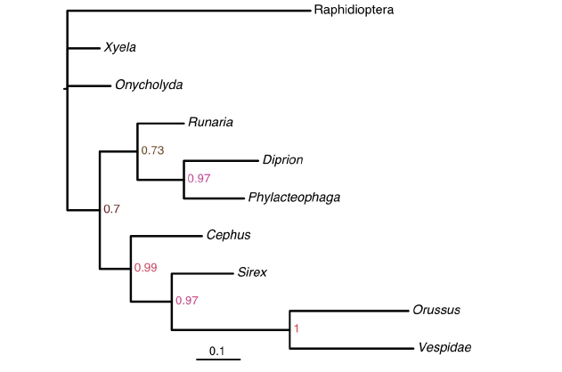
Comparing the non-clock tree (Fig. 5) with the clock trees (Fig. 4), it is obvious that the evolutionary rate is not constant over time. The Xyela and Onycholyda branches evolve much more slowly than the Raphidioptera and Orussus/Vespidae clade, and there are indeed dramatic rate changes between adjacent branches. In this case, the IGR relaxed clock model is more suitable than the autocorrelated TK02 model, and it is not reasonable to assume a strict clock model. Apart from these perspectives, a more statistically rigorous model selection procedure (e.g., using reversible-jump MCMC or marginal likelihood) needs to be carried out in future studies.
Fig. 5
 新窗口打开|下载原图ZIP|生成PPT
Fig. 5Majority-rule consensus tree of extant taxa from a non-clock analysis under the gamma-Dirichlet priorThe branch lengths are measured by expected substitutions per site
The numbers at the internal nodes are the posterior probabilities of the corresponding clades
In conclusion, this study provides a brief overview and comparison of total-evidence dating and node dating analyses, and demonstrates the functionality of MrBayes using a truncated dataset of Hymenoptera. For the analyses and discussion using the full data, please see Ronquist et al. (2012a) and Zhang et al. (2016).
Acknowledgements
I sincerely thank Johan Nylander for valuable discussions and for organizing a workshop of MrBayes using this tutorial in Stockholm, Sweden. I am grateful to Xijun Ni and Rachel C. M. Warnock for insightful review comments. Zhang Chi is supported by the 100 Young Talents Program of Chinese Academy of Sciences and partly supported by the Strategic Priority Research Program of Chinese Academy of Sciences (XDB26000000).参考文献 原文顺序
文献年度倒序
文中引用次数倒序
被引期刊影响因子
PMID [本文引用: 1]

Bayesian estimation of phylogeny is based on the posterior probability distribution of trees. Currently, the only numerical method that can effectively approximate posterior probabilities of trees is Markov chain Monte Carlo (MCMC). Standard implementations of MCMC can be prone to entrapment in local optima. Metropolis coupled MCMC [(MC)(3)], a variant of MCMC, allows multiple peaks in the landscape of trees to be more readily explored, but at the cost of increased execution time.This paper presents a parallel algorithm for (MC)(3). The proposed parallel algorithm retains the ability to explore multiple peaks in the posterior distribution of trees while maintaining a fast execution time. The algorithm has been implemented using two popular parallel programming models: message passing and shared memory. Performance results indicate nearly linear speed improvement in both programming models for small and large data sets.
DOIURL [本文引用: 1]
DOIURL [本文引用: 1]
DOIURL [本文引用: 1]
DOIURL [本文引用: 1]
DOIURL [本文引用: 1]
DOIURL [本文引用: 1]
DOIURL [本文引用: 2]
PMID [本文引用: 2]
The molecular clock hypothesis remains an important conceptual and analytical tool in evolutionary biology despite the repeated observation that the clock hypothesis does not perfectly explain observed DNA sequence variation. We introduce a parametric model that relaxes the molecular clock by allowing rates to vary across lineages according to a compound Poisson process. Events of substitution rate change are placed onto a phylogenetic tree according to a Poisson process. When an event of substitution rate change occurs, the current rate of substitution is modified by a gamma-distributed random variable. Parameters of the model can be estimated using Bayesian inference. We use Markov chain Monte Carlo integration to evaluate the posterior probability distribution because the posterior probability involves high dimensional integrals and summations. Specifically, we use the Metropolis-Hastings-Green algorithm with 11 different move types to evaluate the posterior distribution. We demonstrate the method by analyzing a complete mtDNA sequence data set from 23 mammals. The model presented here has several potential advantages over other models that have been proposed to relax the clock because it is parametric and does not assume that rates change only at speciation events. This model should prove useful for estimating divergence times when substitution rates vary across lineages.
DOIURL [本文引用: 1]
DOIURL [本文引用: 2]
PMID [本文引用: 1]
Evolutionary biologists have adopted simple likelihood models for purposes of estimating ancestral states and evaluating character independence on specified phylogenies; however, for purposes of estimating phylogenies by using discrete morphological data, maximum parsimony remains the only option. This paper explores the possibility of using standard, well-behaved Markov models for estimating morphological phylogenies (including branch lengths) under the likelihood criterion. An important modification of standard Markov models involves making the likelihood conditional on characters being variable, because constant characters are absent in morphological data sets. Without this modification, branch lengths are often overestimated, resulting in potentially serious biases in tree topology selection. Several new avenues of research are opened by an explicitly model-based approach to phylogenetic analysis of discrete morphological data, including combined-data likelihood analyses (morphology + sequence data), likelihood ratio tests, and Bayesian analyses.
DOIURL [本文引用: 1]
DOIURL [本文引用: 1]
DOIURL [本文引用: 1]
DOIURL [本文引用: 3]
PMID [本文引用: 1]
MrBayes 3 performs Bayesian phylogenetic analysis combining information from different data partitions or subsets evolving under different stochastic evolutionary models. This allows the user to analyze heterogeneous data sets consisting of different data types-e.g. morphological, nucleotide, and protein-and to explore a wide variety of structured models mixing partition-unique and shared parameters. The program employs MPI to parallelize Metropolis coupling on Macintosh or UNIX clusters.
DOIURL [本文引用: 5]
DOIURL [本文引用: 1]
DOIURL [本文引用: 1]
DOIURL [本文引用: 2]
DOIURL [本文引用: 1]
DOIURL [本文引用: 1]
PMID [本文引用: 1]
Knowledge of the pattern of nucleotide substitution is important both to our understanding of molecular sequence evolution and to reliable estimation of phylogenetic relationships. The method of parsimony analysis, which has been used to estimate substitution patterns in real sequences, has serious drawbacks and leads to results difficult to interpret. In this paper a model-based maximum likelihood approach is proposed for estimating substitution patterns in real sequences. Nucleotide substitution is assumed to follow a homogeneous Markov process, and the general reversible process model (REV) and the unrestricted model without the reversibility assumption are used. These models are also applied to examine the adequacy of the model of Hasegawa et al. (J. Mol. Evol. 1985;22:160-174) (HKY85). Two data sets are analyzed. For the psi eta-globin pseudogenes of six primate species, the REV models fits the data much better than HKY85, while, for a segment of mtDNA sequences from nine primates, REV cannot provide a significantly better fit than HKY85 when rate variation over sites is taken into account in the models. It is concluded that the use of the REV model in phylogenetic analysis can be recommended, especially for large data sets or for sequences with extreme substitution patterns, while HKY85 may be expected to provide a good approximation. The use of the unrestricted model does not appear to be worthwhile.
PMID [本文引用: 1]
Two approximate methods are proposed for maximum likelihood phylogenetic estimation, which allow variable rates of substitution across nucleotide sites. Three data sets with quite different characteristics were analyzed to examine empirically the performance of these methods. The first, called the "discrete gamma model," uses several categories of rates to approximate the gamma distribution, with equal probability for each category. The mean of each category is used to represent all the rates falling in the category. The performance of this method is found to be quite good, and four such categories appear to be sufficient to produce both an optimum, or near-optimum fit by the model to the data, and also an acceptable approximation to the continuous distribution. The second method, called "fixed-rates model", classifies sites into several classes according to their rates predicted assuming the star tree. Sites in different classes are then assumed to be evolving at these fixed rates when other tree topologies are evaluated. Analyses of the data sets suggest that this method can produce reasonable results, but it seems to share some properties of a least-squares pairwise comparison; for example, interior branch lengths in nonbest trees are often found to be zero. The computational requirements of the two methods are comparable to that of Felsenstein's (1981, J Mol Evol 17:368-376) model, which assumes a single rate for all the sites.
DOIURL [本文引用: 1]
DOIURL [本文引用: 4]
DOIURL [本文引用: 7]
