Jiaxin Qi^,, Hongli An^,, Peng JinCollege of Sciences, Nanjing Agricultural University, Nanjing, 210095, China

Received:2021-08-7Revised:2021-10-10Accepted:2021-10-13Online:2021-11-23


Abstract
The (2+1)-dimensional Boiti–Leon–Manna–Pempinelli (BLMP) equation is an important integrable model. In this paper, we obtain the breather molecule, the breather-soliton molecule and some localized interaction solutions to the BLMP equation. In particular, by employing a compound method consisting of the velocity resonance, partial module resonance and degeneration of the breather techniques, we derive some interesting hybrid solutions mixed by a breather-soliton molecule/breather molecule and a lump, as well as a bell-shaped soliton and lump. Due to the lack of the long wave limit, it is the first time using the compound degeneration method to construct the hybrid solutions involving a lump. The dynamical behaviors and mathematical features of the solutions are analyzed theoretically and graphically. The method introduced can be effectively used to study the wave solutions of other nonlinear partial differential equations.
Keywords： Boiti–Leon–Manna–Pempinelli equation;module resonance;velocity resonance solutions;breather molecules;interaction solutions


PDF (1085KB)MetadataMetricsRelated articlesExportEndNote|Ris|BibtexFavorite
Cite this article
Jiaxin Qi, Hongli An, Peng Jin. Breather molecules and localized interaction solutions in the (2+1)-dimensional BLMP equation. Communications in Theoretical Physics, 2021, 73(12): 125005- doi:10.1088/1572-9494/ac2f2b

1. Introduction

The (2+1)-dimensional Boiti–Leon–Manna–Pempinelli (BLMP) equation under consideration is an adopted form of:(1.1)$\begin{eqnarray}{u}_{{yt}}+{u}_{{xxxy}}-3{u}_{x}{u}_{{xy}}-3{u}_{{xx}}{u}_{y}=0,\end{eqnarray}$which has been widely used in fluids, plasmas, nano-materials and other physical and engineering phenomena [1]. Due to its wide applications, the BLMP equation has been extensively and intensively studied in many papers. For example, based on the binary Bell polynomials, the Lax pair and Bäcklund transformation were derived in [2]. Ghoston solutions were constructed by means of the multi-linear variable separation approach in [3]. Jacobi periodic wave solutions were discussed via introducing Jacobi elliptic functions [4] and subsequently by the extended homoclinic test approach [5]. While, multiple wave and positive compelexiton solutions were constructed in [6]. The D'Alembert wave and a soliton molecule solution were analyzed in [7] and various localized wave solutions were derived in [8]. There are also other kinds of solutions that were obtained for the (2+1)-dimensional and (3+1)-dimensional BLMP equation (see references [9–15]).

Nowadays, investigations into breather molecules is a hot topic. The breather molecule is a special kind of soliton molecule, which displays periodic structure in a certain direction and owns molecule-like behaviors. The latter was originally presented by Akhmediev et al [16] and observed by Stratmann et al in the experiment [17]. Investigations show that soliton molecules have many appealing features and been widely used in plasmas physics, optics, Bose–Einstein condensates and fluid dynamics [18–21]. When a complex conjugate constraint is introduced, the soliton molecule will turn to the breather molecule. The breather molecule has been observed in mode-locked fiber laser experiments [22]. Recently, Lou et al proposed the velocity resonance and module resonance principle and therefore some breather molecules are obtained [23, 24]. The work of Lou's motivates many experts to devote themselves to seeking soliton and breather molecules in various physical models. Up to now, the soliton and breather molecules are constructed for the Sawada–Kotera equation [25], the complex mKdV equation [26], the fifth-order KdV equation [27] and the Sharma–Tasso–Olver–Burgers equation etc [28–30]. Therefore, it would be of interest to seek molecule solutions in other physical models.

Inspections show that no investigations have been carried on breather molecules of the (2+1)-dimensional BLMP equation. Not much work has been done on the interaction solutions of breather-molecule-types. To the best of our knowledge, no work has been carried out on the interactions between a breather molecule or breather-soliton molecule and lumps, yet. We notice that the special form of the BLMP equation makes the long wave limit lose its power to derive the molecule interaction solutions involving lumps. However, such solutions seem to have wider applications in the real world. Therefore, it is worth considering whether alternative methods exist that lead to these solutions.

To summarise, in this paper we would like to investigate the breather molecule and interaction solutions of the the BLMP equation. Our work begins with a logarithmic transformation. Under the transformation, N-soliton solutions of the BLMP equation are constructed. Then, the partial velocity resonance, the module resonance principle and a partial degeneration of the breather technique are employed, thereby the breather molecule, breather-soliton molecule and some hybrid solutions (such as the interactions between a breather molecule and lump, between a breather-soliton molecule and lump etc.) are obtained. We would like to stress that it is the first time using the degeneration method to obtain the interaction solutions between molecules and a lump. To shed light on the dynamical behaviors the solutions may posses, numerical simulations and illustrative tables are given, which indicate that the types of solutions and their features are intimately related to the restricted conditions.

2. N-soliton solutions of the (2+1)-dimensional BLMP equation

In order to obtain the breather molecule and related interaction solutions, we need to construct the N-soliton solutions of the (2+1)-dimensional BLMP equation first. For that purpose, a special transformation is introduced via(2.1)$\begin{eqnarray}u=2{\left(\mathrm{ln}f\right)}_{x},\end{eqnarray}$so that the equation (1.1) can be rewritten as the Hirota bilinear form(2.2)$\begin{eqnarray}({D}_{y}{D}_{t}+{D}_{x}^{3}{D}_{y})f\cdot f=0,\end{eqnarray}$where D_x, D_y and D_t are the bilinear derivative operators defined via(2.3)$\begin{eqnarray}\begin{array}{l}{D}_{x}^{\alpha }{D}_{y}^{\beta }{D}_{t}^{\gamma }(f\cdot g)={\left({\partial }_{x}-{\partial }_{x^{\prime} }\right)}^{\alpha }{\left({\partial }_{y}-{\partial }_{y^{\prime} }\right)}^{\beta }\\ {\left({\partial }_{t}-{\partial }_{t^{\prime} }\right)}^{\gamma }f(x,y,t)g(x^{\prime} ,y^{\prime} ,t^{\prime} ){| }_{x^{\prime} =x,y^{\prime} =y,t^{\prime} =t},\end{array}\end{eqnarray}$where α, β and γ are non-negative integers denoting the orders of bilinear derivative operators.

According to the Hirota bilinear method [31], the N-soliton solutions to the BLMP equation are derived(2.4)$\begin{eqnarray}\begin{array}{l}u=2{\left(\mathrm{ln}f\right)}_{x}\\ \,=\,2\left[\mathrm{ln}\displaystyle \sum _{\mu =0,1}\right.{\left.\exp \left(\displaystyle \sum _{i=1}^{N}{\mu }_{i}{\eta }_{i}+\displaystyle \sum _{i\lt j}^{N}{\mu }_{i}{\mu }_{j}{A}_{{ij}}\right)\right]}_{x},\end{array}\end{eqnarray}$where(2.5)$\begin{eqnarray}\begin{array}{rcl}{\omega }_{i}&=&-{k}_{i}^{2},\quad \quad {\eta }_{i}={k}_{i}(x+{p}_{i}y+{\omega }_{i}t)+{\eta }_{i}^{0},\\ {A}_{{ij}}&=&\displaystyle \frac{({k}_{i}-{k}_{j})({k}_{i}{p}_{i}-{k}_{j}{p}_{j})}{({k}_{i}+{k}_{j})({k}_{i}{p}_{i}+{k}_{j}{p}_{j})},\quad \quad i,j=1,2,\cdots ,\,N.\end{array}\end{eqnarray}$In the above k_i, p_i, ω_i and ${\eta }_{i}^{0}$ are arbitrary constants. While ∑_μ=0,1 means summation over all possible combinations of μ_i, μ_j = 0, 1.

3. A breather-soliton molecule and some related interaction solutions

In this section, we show that by employing the partial velocity resonance principle and module resonance of two waves, a breather-soliton molecule and four kinds of interactions solutions are obtained. Interestingly, when the partial degeneration of the breather technique is additionally adopted, two new kinds of resonant solutions mixed by a breather-soliton molecule and a lump as well as a bell-shaped soliton and a lump are derived. We emphasize that due to the special form of the BLMP equation, the long wave limit loses its power. Therefore, it is the first time to use the degeneration of breathers to generate the interaction molecule solutions involving a lump.

To construct the breather-soliton molecule and interaction solutions, we need to set N = 3 + P (P = 0, 1, ⋯). On imposing the complex conjugate constraints to {k_i, p_i} (i = 1, 2):(3.1)$\begin{eqnarray}\begin{array}{l}{k}_{1}={k}_{2}^{* }={k}_{1r}+{\rm{i}}{k}_{1i},\\ {p}_{1}={p}_{2}^{* }\,=\,{p}_{1r}+{\rm{i}}{p}_{1i},\end{array}\end{eqnarray}$and introducing the module resonance as well as the partial velocity resonance principle:(3.2)$\begin{eqnarray}\begin{array}{l}\displaystyle \frac{{k}_{1r}}{{k}_{3}}=\displaystyle \frac{{k}_{1r}{p}_{1r}-{k}_{1i}{p}_{1i}}{{k}_{3}{p}_{3}}\\ =\displaystyle \frac{{k}_{1r}^{3}-3{k}_{1r}{k}_{1i}^{2}}{{k}_{3}^{3}},\end{array}\end{eqnarray}$then different kinds of solutions can be obtained wherein the types of the solutions and their behaviors depends on the values of P and parameters of {k_i, p_i}. The details are discussed as follows:

Case 1: Considering P = 0. When insertion of (3.1) and (3.2) into (2.4), one can easily obtain a resonant solution of the breather-soliton molecule ({BSM}). To detect the dynamical behaviors of such a solution, we present the corresponding numerical simulations in figure 1. The figure illustrates that the soliton and the breather are parallel to each other, which is just because of the complex conjugate restriction (3.1) and module resonance technique adopted in (3.2). With the time evolution, the distance between the soliton and breather remains unchanged.

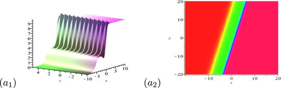
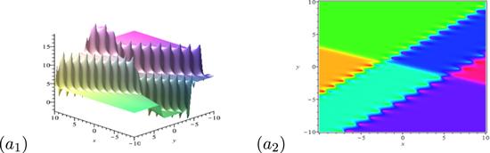
Figure 1.

New window|Download| PPT slide
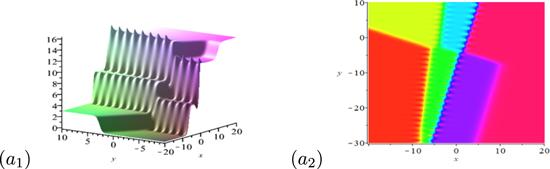
Figure 1.Dynamical behaviors of the breather-soliton molecule. The parameters are given by k_1r = 1.56, k_1i = 0.25, k₃ = 1.5, p_1r = 0.5, p_1i = 4.68, p₃ = −0.25.


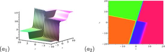
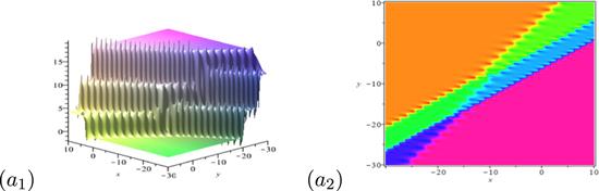
Case 2: Taking P = 1. OBy making similar analysis to Case 1, one can derive an interaction solution mixed by a breather-soliton molecule and a bell-shaped soliton ({BSM, S}). It is necessary to point out that: the {BSM, S} described in figure 2 exhibits quite different dynamical behaviors to the {BSM} given in figure 1, although the same techniques are used. Figure 2 shows that the breather parallels to one of the solitons (labelled as 3rd-soliton) to form the breather-soliton molecule and then interacts with the other soliton (labelled as 4th-soliton). Unlike Case 1, the distance between the breather-soliton and the 4th-soliton changes over time. Therefore, the interactions of the {BSM, S} are inelastic.

Figure 2.

New window|Download| PPT slide
Figure 2.Dynamical behaviors of the hybrid solution between a breather-soliton and a bell-shaped soliton. The parameters are chosen as ${k}_{1r}=\sqrt{7}$, k_1i = 1, k₃ = 2, k₄ = 2, ${p}_{1r}=\tfrac{1}{2}$, ${p}_{1i}=\tfrac{3\sqrt{7}}{4}$, ${p}_{3}=-\tfrac{1}{4}$, p₄ = 4.


Case 3: Setting P = 2. If we additionally impose the complex conjugate conditions to the parameters {k_i, p_i}(i = 4, 5) via(3.3)$\begin{eqnarray}\begin{array}{l}{k}_{4}={k}_{5}^{* }={k}_{4r}+{\rm{i}}{k}_{4i},\\ {p}_{4}={p}_{5}^{* }={p}_{4r}+{\rm{i}}{p}_{4i},\end{array}\end{eqnarray}$so that the 4th- and 5th-solitons form one breather (labelled as 2nd-breather). Combining it with the relations (3.1) and (3.2) produces a localized interaction solution mixed by a breather-soliton and breather ({BSM, B}) whose dynamical behaviors are displayed in figure 3.

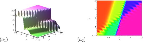
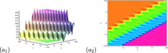
Figure 3.

New window|Download| PPT slide
Figure 3.Dynamical behaviors of the hybrid solution mixed by a breather-soliton molecule and breather.


In [32], it is revealed that a partial degeneration of the breather can lead to a lump. Here, we shall combine the degeneration technique with the module resonance principle to construct the interaction solution mixed by a breather-soliton molecule and lump. Thus, we need to know the periodicity of the related breather first.

Calculations show that the periodicity of the 2nd-breather along the x direction is ${T}_{[x]}=| \tfrac{2\pi ({p}_{4r}{k}_{4r}-{p}_{4i}{k}_{4i})}{{p}_{4i}({k}_{4r}^{2}+{k}_{4i}^{2})}| $ and the periodicity along the y direction is ${T}_{[y]}=| \tfrac{2\pi {k}_{4r}}{{p}_{4i}({k}_{4r}^{2}+{k}_{4i}^{2})}| $. Therefore, the composite periodicity of the 2nd-breather is:(3.4)$\begin{eqnarray}\begin{array}{l}T=\sqrt{{T}_{[x]}^{2}+{T}_{[y]}^{2}}=\displaystyle \frac{2\pi }{| {p}_{4i}| ({k}_{4r}^{2}+{k}_{4i}^{2})}\\ \sqrt{{\left({p}_{4r}{k}_{4r}-{p}_{4i}{k}_{4i}\right)}^{2}+{k}_{4r}^{2}}.\end{array}\end{eqnarray}$If setting T → 0, then the 2nd-breather will degenerate into a lump. Accordingly, a new kind of interaction solution between a breather-soliton molecule and lump ({BSM, L}) is obtained. To fully show the detailed degeneration process, we take a special solution as an illustrative example. Numerical simulations are depicted in figure 4. From these pictures one can easily see that the 2nd-breather in the mixed solution successively degenerates into the lump and then the interaction solution of {BSM, L} is generated.

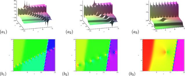
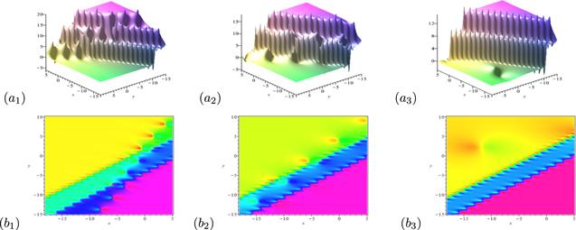
Figure 4.

New window|Download| PPT slide
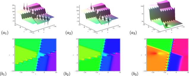
Figure 4.The degeneration process of the solution mixed by a breather-soliton molecule and lump from {BSM, B}. The parameters are chosen as flows: k_1r = 4, k_1i = 2, k₃ = 2, p_1r = 0.17, p_1i = 0.83, p₃ = − 0.25, p_4r = 0.03, p_4i = 1.5. (a₁)(b₁) k_4r = 1, k_4i = 2; (a₂)(b₂) ${k}_{4r}=\tfrac{2}{5}$, k_4i = 1; (a₃)(b₃) ${k}_{4r}=\tfrac{1}{5}$, ${k}_{4i}=\tfrac{1}{8}$.


Case 4: When P = 3, if we only require a pair of complex conjugate conditions (3.1) and (3.3), by employing the module resonance technique, we derive an interaction solution mixed by a breather-soliton molecule, one breather and a bell-shaped soliton ({BSM, B, S}), which is exhibited in figure 5. However, if partial degenerating of the breather technique mentioned in the above is employed, then the {BSM, B, S} will degenerate to an interaction solution composed by a breather-soliton molecule and a lump and bell-shaped soliton ({BSM, L, S}), which is shown in figure 6.

Figure 5.

New window|Download| PPT slide
Figure 5.Dynamical behaviors of the interaction solution composed by a breather-soliton molecule, a breather and a soliton. The parameters are selected as k_1r = 1.32, k_1i = 0.25, k₃ = 1.5, k_4r = 1.73, k_4i = 0.5, k₆ = 1.5, p_1r = 0.5, p_1i = 3.17, p₃ = −0.25, p_4r = 0.33, p_4i =2.02, p₆ = 4.

Figure 6.

New window|Download| PPT slide
Figure 6.The degeneration process of the solution mixed by a breather-soliton molecule, a lump and a soliton from {BSM, B, S}. The parameters are chosen as flows: k_1r = 1.732, k_1i = 0.5, k₃ = 1.5, p_1r = 0.33, p_1i = 2.02, p₃ = −0.25, p_4r = 0.08, p_4i = 4, k₆ = 1.5, p₆ = 4. (a₁)(b₁) k_4r = 0.8, k_4i = 0.8; (a₂)(b₂) k_4r = 0.5, k_4i = 0.8; (a₃)(b₃) k_4r = 0.02, k_4i = 0.2.


Interestingly, if we set the additional P solitons to satisfy the module resonance principle via(3.5)$\begin{eqnarray}\begin{array}{l}{k}_{4}={k}_{5}^{* }={k}_{4r}+{\rm{i}}{k}_{4i},\\ {p}_{4}={p}_{5}^{* }\,=\,{p}_{4r}+{\rm{i}}{p}_{4i},\\ \displaystyle \frac{{k}_{4r}}{{k}_{6}}=\displaystyle \frac{{k}_{4r}{p}_{4r}-{k}_{4i}{p}_{4i}}{{k}_{6}{p}_{6}}=\displaystyle \frac{{k}_{4r}^{3}-3{k}_{4r}{k}_{4i}^{2}}{{k}_{6}^{3}},\end{array}\end{eqnarray}$then the 6 solitons turn to form a mixed solution between two different breather-soliton molecules ({BSM, BSM}) and the dynamical behaviors are simulated in figure 7. From this figure, we can see that there are two different molecules that form the bounded state.

Figure 7.

New window|Download| PPT slide
Figure 7.Dynamical behaviors of the interaction solution mixed by two different breather-soliton molecules. The parameters are given by k_1r = 1.32, k_1i = 0.25, k₃ = 1.5, k_4r = 1.73, k_4i = 0.5, k₆ = 1.25, p_1r = 0.5, p_1i = 3.17, p₃ = −0.25, p_4r = 0.33, p_4i = 2.02, p₆ = −0.1.


Now, we give the related mathematical features in order to obtain the breather-soliton molecule and interaction solutions when N = 3 + P. Details are given in table 1. The first column in the table describes the numbers of N and P. While the second and third columns show the types of the solutions and corresponding different parameters as well as restricted conditions.


Table 1.
Table 1.Breather-soliton molecule and interaction solutions.

N = 3 + P	Name of the solution	Restriction conditions
P = 0	{BSM}	${k}_{1}={k}_{2}^{* }={k}_{1r}+{\rm{i}}{k}_{1i},\quad {p}_{1}={p}_{2}^{* }\,=\,{p}_{1r}+{\rm{i}}{p}_{1i}$,
		$\tfrac{{k}_{1r}}{{k}_{3}}=\tfrac{{k}_{1r}\ {p}_{1r}-{k}_{1i}\ {p}_{1i}}{{k}_{3}\ {p}_{3}}=\tfrac{{k}_{1r}^{3}-3{k}_{1r}\ {k}_{1i}^{2}}{{k}_{3}^{3}}$
P = 1	{BSM, S}	the same as above
P = 2	{BSM, B}	${k}_{1}={k}_{2}^{* }={k}_{1r}+{\rm{i}}{k}_{1i},\quad {p}_{1}={p}_{2}^{* }\,=\,{p}_{1r}+{\rm{i}}{p}_{1i}$,
		${k}_{4}={k}_{5}^{* }={k}_{4r}+{\rm{i}}{k}_{4i},\quad {p}_{4}={p}_{5}^{* }={p}_{4r}+{\rm{i}}{p}_{4i}$
		$\tfrac{{k}_{1r}}{{k}_{3}}=\tfrac{{k}_{1r}\ {p}_{1r}-{k}_{1i}\ {p}_{1i}}{{k}_{3}\ {p}_{3}}=\tfrac{{k}_{1r}^{3}-3{k}_{1r}\ {k}_{1i}^{2}}{{k}_{3}^{3}}$,
P = 2	{BSM, L}	${k}_{1}={k}_{2}^{* }={k}_{1r}+{\rm{i}}{k}_{1i},\quad {p}_{1}={p}_{2}^{* }\,=\,{p}_{1r}+{\rm{i}}{p}_{1i}$,
		${k}_{4}={k}_{5}^{* }={k}_{4r}+{\rm{i}}{k}_{4i},\quad {p}_{4}={p}_{5}^{* }={p}_{4r}+{\rm{i}}{p}_{4i}$,
		$\tfrac{{k}_{1r}}{{k}_{3}}=\tfrac{{k}_{1r}\ {p}_{1r}-{k}_{1i}\ {p}_{1i}}{{k}_{3}\ {p}_{3}}=\tfrac{{k}_{1r}^{3}-3{k}_{1r}\ {k}_{1i}^{2}}{{k}_{3}^{3}}$,
		${k}_{4r}^{2}+{k}_{4i}^{2}\to 0$
P = 3	{BSM, B, S}	the same as what's used in {BSM, B}
P = 3	{BSM, L, S}	the same as what's used in {BSM, L}
P = 3	{BSM, BSM}	${k}_{1}={k}_{2}^{* }={k}_{1r}+{\rm{i}}{k}_{1i},\quad {p}_{1}={p}_{2}^{* }\,=\,{p}_{1r}+{\rm{i}}{p}_{1i}$,
		${k}_{4}={k}_{5}^{* }={k}_{4r}+{\rm{i}}{k}_{4i},\quad {p}_{4}={p}_{5}^{* }\,=\,{p}_{4r}+{\rm{i}}{p}_{4i}$,
		$\tfrac{{k}_{1r}}{{k}_{3}}=\tfrac{{k}_{1r}\ {p}_{1r}-{k}_{1i}\ {p}_{1i}}{{k}_{3}\ {p}_{3}}=\tfrac{{k}_{1r}^{3}-3{k}_{1r}\ {k}_{1i}^{2}}\ {{k}_{3}^{3}}$,
		$\tfrac{{k}_{4r}}{{k}_{6}}=\tfrac{{k}_{4r}\ {p}_{4r}-{k}_{4i}\ {p}_{4i}}{{k}_{6}\ {p}_{6}}=\tfrac{{k}_{4r}^{3}-3{k}_{4r}\ {k}_{4i}^{2}}{{k}_{6}^{3}}$

New window|CSV

4. A breather molecule and some related interaction solutions

In this section, by using the module resonance of four waves and partial degeneration of breather techniques, a breather molecule and five different resonant solutions are derived. Their dynamical behaviors and mathematical features are discussed.

To obtain the breather molecule and related interaction solutions, it requires to set N = 4 + P. Meanwhile, two pairs of solitons need to satisfy the conjugate constraints:(4.1)$\begin{eqnarray}\begin{array}{l}{k}_{1}={k}_{2}^{* }={k}_{1r}+{\rm{i}}{k}_{1i},\quad {p}_{1}={p}_{2}^{* }\,=\,{p}_{1r}+{\rm{i}}{p}_{1i},\\ \quad {k}_{3}={k}_{4}^{* }={k}_{3r}+{\rm{i}}{k}_{3i},\quad {p}_{3}={p}_{4}^{* }={p}_{3r}+{\rm{i}}{p}_{3i},\end{array}\end{eqnarray}$Now a resonant technique that is different to the one used in (3.2) is employed:(4.2)$\begin{eqnarray}\begin{array}{l}\displaystyle \frac{{k}_{1r}}{{k}_{3r}}=\displaystyle \frac{{k}_{1r}{p}_{1r}-{k}_{1i}{p}_{1i}}{{k}_{3r}{p}_{3r}-{k}_{3i}{p}_{3i}}\\ =\ \displaystyle \frac{{k}_{1r}^{3}-3{k}_{1r}{k}_{1i}^{2}}{{k}_{3r}^{3}-3{k}_{3r}{k}_{3i}^{2}},\end{array}\end{eqnarray}$then many different kinds of localized resonant solutions can be derived. Here, we list five of them.

Case 1: Taking P = 0. On substituting (4.1) and (4.2) into the four solitons expression (2.4), we obtain a kind of solution termed as a breather molecule ({BBM}). Dynamical behaviors of a typical {BBM} are shown in figure 8. Although the two breathers have different periods, they are parallel to each other and form a bounded state (breather molecule) due to the resonance condition introduced in (4.2). Such a bounded state renders the distance and velocity between the two breathers unchanged.

Figure 8.

New window|Download| PPT slide
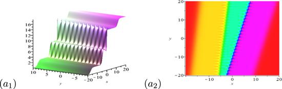
Figure 8.Dynamical behaviors of the breather molecule. The parameters are set as k_1r = 1.73, k_1i = 1.25, k_3r = 1.39, k_3i = 1.10, p_1r = 0.73, p_1i = 3, p_3r = 0.73 and p_3i = 2.73.


Case 2: Considering P = 1. When adopting the analogous technique mentioned in the above to the five-solitons, we obtain an interaction solution mixed by a breather molecule and a bell-shaped soliton ({BBM, S}). Dynamical behaviors of their interactions are traced in figure 9.

Figure 9.

New window|Download| PPT slide
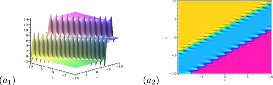
Figure 9.Dynamical behaviors of the mixed solution by a breather molecule and soliton. The parameters are set as k_1r = 1.73, k_1i = 1.25, k_3r = 1.39, k_3i = 1.10, k5 = 2, p_1r = 0.73, p_1i = 3, p_3r = 0.73 , p_3i = 2.73 and p₅ = 3.23.


Case 3: Considering P = 2. When the following complex conjugate restriction is introduced via(4.3)$\begin{eqnarray}{k}_{5}={k}_{6}^{* }={k}_{5r}+{\rm{i}}{k}_{5i},\quad {p}_{5}={p}_{6}^{* }={p}_{5r}+{\rm{i}}{p}_{5i},\end{eqnarray}$to the 5th- and 6th-solitons, then the two solitons constitute a breather (labelled as the 3rd-breather). On insertion of (4.1) and (4.2) into the expression (2.4), an interaction solution between a breather molecule and breather ({BBM, B}) can be derived, whose dynamical behaviors are exhibited in figure 10.

Figure 10.

New window|Download| PPT slide
Figure 10.Dynamical behaviors of the interaction solution between a breather molecule and breather. The parameters are chosen as: k₁ = 1.73 + 1.25i, k₃ = 1.39 + 1.10i, k₅ = 1.04 + 0.6i, p₁ = 0.73 + 3i, p₃ = 0.73 + 2.73i, p₅ = 0.73 + 2.73i.


Remarkably, we note that if we also require the breather molecule and the 3rd-breather to satisfy the resonance principle given by:(4.4)$\begin{eqnarray}\displaystyle \frac{{k}_{1r}}{{k}_{5r}}=\displaystyle \frac{{k}_{1r}{p}_{1r}-{k}_{1i}{p}_{1i}}{{k}_{5r}{p}_{5r}-{k}_{5i}{p}_{5i}}=\displaystyle \frac{{k}_{1r}^{3}-3{k}_{1r}{k}_{1i}^{2}}{{k}_{5r}^{3}-3{k}_{5r}{k}_{5i}^{2}},\end{eqnarray}$then, a kind of resonant solution termed as a breather-breather-breather molecule ({BBBM}) is obtained and the dynamical behaviors are displayed in figure 11. From the figure, we can see that the 3rd-breather in figure 11 retains the same state as the other two breathers, which is different from what is shown in figure 10.

Figure 11.

New window|Download| PPT slide
Figure 11.Dynamical behaviors of a breather-breather-breather molecule. The parameters are chosen as:k₁ = 1.73 + 1.25i, k₃ = 1.39 + 1.10i, k₅ = 1.04 + 0.96i, p₁ = 0.73 + 3i, p₃ = 0.73 + 1.73i, p₅ = 0.73 + 2.34i.


Otherwise, we turn to the solution of {BBM, B}, in which the 3rd-breather satisfies the complex conjugate condition given in (4.3). Calculations show that its periodicity is described by(4.5)$\begin{eqnarray}\begin{array}{l}T=\sqrt{{T}_{[x]}^{2}+{T}_{[y]}^{2}}\\ \,=\,\displaystyle \frac{2\pi }{| {p}_{5i}| ({k}_{5r}^{2}+{k}_{5i}^{2})}\sqrt{{\left({p}_{5r}{k}_{5r}-{p}_{5i}{k}_{5i}\right)}^{2}+{k}_{5r}^{2}}.\end{array}\end{eqnarray}$Then, by applying the partial degeneration technique and the resonant principle (4.2) to {BBM, B} when T → 0, we obtain a mixed solution consisting of a breather molecule and lump ({BBM, L}). The detailed degeneration process can be seen in figure 12.

Figure 12.

New window|Download| PPT slide
Figure 12.The degeneration process of the solution mixed by a breather molecule and lump from {BB, B}. The parameters are chosen as flows: k_1r = 1.73, k_1i = 1.25, k_3r = 1.39, k_3i = 1.10, p_1r = 0.73, p_1i = 3, p_3r = 0.73, p_3i = 2.73, p_5r = 0.15, p_5i = 1.5. (a₁)(b₁) k_5r = 1, k_5i = 0.6; (a₂)(b₂) k_5r = 0.5, k_5i = 0.4; (a₃)(b₃) k_5r = 0.1, k_5i = 0.3.


Now, we summarize some restriction conditions to obtain the breather molecule and various interaction solutions when N = 4 + P. Details can be seen in table 2.


Table 2.
Table 2.Breather molecule and interaction solutions.

N = 4 + P	Name of the solution	Restriction conditions
P = 0	{BBM}	${k}_{1}={k}_{2}^{* }={k}_{1r}+{\rm{i}}{k}_{1i},\quad {p}_{1}={p}_{2}^{* }\,=\,{p}_{1r}+{\rm{i}}{p}_{1i}$,
		${k}_{3}={k}_{4}^{* }={k}_{3r}+{\rm{i}}{k}_{3i},\quad {p}_{3}={p}_{4}^{* }={p}_{3r}+{\rm{i}}{p}_{3i}$,
		$\tfrac{{k}_{1r}}{{k}_{3r}}=\tfrac{{k}_{1r}\ {p}_{1r}-{k}_{1i}\ {p}_{1i}}{{k}_{3r}\ {p}_{3r}-{k}_{3i}\ {p}_{3i}}=\tfrac{{k}_{1r}^{3}-3{k}_{1r}\ {k}_{1i}^{2}}{{k}_{3r}^{3}-3{k}_{3r}\ {k}_{3i}^{2}}$
P = 1	{BBM, S}	the same as above
P = 2	{BBM, B}	${k}_{1}={k}_{2}^{* }={k}_{1r}+{\rm{i}}{k}_{1i},\quad {p}_{1}={p}_{2}^{* }\,=\,{p}_{1r}+{\rm{i}}{p}_{1i}$,
		${k}_{3}={k}_{4}^{* }={k}_{3r}+{\rm{i}}{k}_{3i},\quad {p}_{3}={p}_{4}^{* }={p}_{3r}+{\rm{i}}{p}_{3i}$,
		$\tfrac{{k}_{1r}}{{k}_{3r}}=\tfrac{{k}_{1r}\ {p}_{1r}-{k}_{1i}\ {p}_{1i}}{{k}_{3r}\ {p}_{3r}-{k}_{3i}\ {p}_{3i}}=\tfrac{{k}_{1r}^{3}-3{k}_{1r}\ {k}_{1i}^{2}}{{k}_{3r}^{3}-3{k}_{3r}\ {k}_{3i}^{2}}$,
		${k}_{5}={k}_{6}^{* }={k}_{5r}+{\rm{i}}{k}_{5i},\quad {p}_{5}={p}_{6}^{* }={p}_{5r}+{\rm{i}}{p}_{5i}$
P = 2	{BBM, L}	${k}_{1}={k}_{2}^{* }={k}_{1r}+{\rm{i}}{k}_{1i},\quad {p}_{1}={p}_{2}^{* }\,=\,{p}_{1r}+{\rm{i}}{p}_{1i}$,
		${k}_{3}={k}_{4}^{* }={k}_{3r}+{\rm{i}}{k}_{3i},\quad {p}_{3}={p}_{4}^{* }={p}_{3r}+{\rm{i}}{p}_{3i}$,
		${k}_{5}={k}_{6}^{* }={k}_{5r}+{\rm{i}}{k}_{5i},\quad {p}_{5}={p}_{6}^{* }={p}_{5r}+{\rm{i}}{p}_{5i},$
		$\tfrac{{k}_{1r}}{{k}_{3r}}=\tfrac{{k}_{1r}\ {p}_{1r}-{k}_{1i}\ {p}_{1i}}{{k}_{3r}\ {p}_{3r}-{k}_{3i}\ {p}_{3i}}=\tfrac{{k}_{1r}^{3}-3{k}_{1r}\ {k}_{1i}^{2}}{{k}_{3r}^{3}-3{k}_{3r}\ {k}_{3i}^{2}}$,
		${k}_{5r}^{2}+{k}_{5i}^{2}\to 0$
P = 2	{BBBM}	${k}_{1}={k}_{2}^{* }={k}_{1r}+{\rm{i}}{k}_{1i},\quad {p}_{1}={p}_{2}^{* }\,=\,{p}_{1r}+{\rm{i}}{p}_{1i}$,
		${k}_{3}={k}_{4}^{* }={k}_{3r}+{\rm{i}}{k}_{3i},\quad {p}_{3}={p}_{4}^{* }={p}_{3r}+{\rm{i}}{p}_{3i}$,
		${k}_{5}={k}_{6}^{* }={k}_{5r}+{\rm{i}}{k}_{5i},\quad {p}_{5}={p}_{6}^{* }={p}_{5r}+{\rm{i}}{p}_{5i}$,
		$\tfrac{{k}_{1r}}{{k}_{3r}}=\tfrac{{k}_{1r}\ {p}_{1r}-{k}_{1i}\ {p}_{1i}}{{k}_{3r}\ {p}_{3r}-{k}_{3i}\ {p}_{3i}}=\tfrac{{k}_{1r}^{3}-3{k}_{1r}\ {k}_{1i}^{2}}{{k}_{3r}^{3}-3{k}_{3r}\ {k}_{3i}^{2}}$,
		$\tfrac{{k}_{1r}}{{k}_{5r}}=\tfrac{{k}_{1r}\ {p}_{1r}-{k}_{1i}\ {p}_{1i}}{{k}_{5r}\ {p}_{5r}-{k}_{5i}\ {p}_{5i}}=\tfrac{{k}_{1r}^{3}-3{k}_{1r}\ {k}_{1i}^{2}}{{k}_{5r}^{3}-3{k}_{5r}\ {k}_{5i}^{2}}$

New window|CSV

5. Conclusion

In recent years, investigating the breather molecules and soliton molecules, which has been widely used in plasmas physics, optics, Bose–Einstein condensates and fluid dynamics, is a very popular topic. In this paper, we construct the breather molecule, breather-soliton molecule and many related interactions solutions of the BLMP equation. In particular, by using the technique composed by the partial velocity resonance, the module resonance and degenerating the breather, we derive the hybrid solutions mixed by a breather molecule/breather-soliton molecule and a lump/breather/a lump and a bell-shaped soliton. All these solutions, especially the interactions involving lumps are completely new and interesting. Their dynamical behaviors and mathematical structures are discussed in detail. It is necessary to point out that the compound degeneration method introduced here can be effectively used to investigate the interaction solutions involving lumps of nonlinear systems. Based on the importance and wide applications of the breather molecule and the BLMP equation, we hope that such solutions can be helpful for understanding and studying the propagations of nonlinear localized waves.

Acknowledgments

This work is supported by the National Natural Science Foundation of China under Grant No. 11 775 116 and Jiangsu Qinglan high-level talent Project.

Reference View Option By original order
By published year
By cited within times
By Impact factor

[1]Ablowitz M J Clarkson P A 1991 Soliton, Nonlinear Evolution Equations and Inverse Scatting New York Cambridge University Press
[Cited within: 1]

[2]Luo L 2011 Phys. Lett. A 375 1059
DOI:10.1016/j.physleta.2011.01.009 [Cited within: 1]

[3]Tang X Y 2003 Phys. Lett. A 314 286
DOI:10.1016/S0375-9601(03)00873-9 [Cited within: 1]

[4]Bai C J Zhao H 2008 Int. J. mod. Phys. B 22 2407
DOI:10.1142/S021797920803954X [Cited within: 1]

[5]Tang Y N Zai W J 2015 Nonlinear Dyn. 81 249
DOI:10.1007/s11071-015-1986-4 [Cited within: 1]

[6]Hosseini K Ma W X Ansari R Mirzazadeh M Pouyanmehr R Samadani F 2020 Phys. Scripta. 95 065208
DOI:10.1088/1402-4896/ab7fee [Cited within: 1]

[7]Ren B 2021 Commun. Theor. Phys. 73 035003
DOI:10.1088/1572-9494/abda17 [Cited within: 1]

[8]Sun L Qi J X An H L 2020 Commun. Theor. Phys. 72 125009
DOI:10.1088/1572-9494/abbbd8 [Cited within: 1]

[9]Hu L Gao Y T Jia S L Su J J Deng G F 2019 Mod. Phys. Lett. B 33 1950376
DOI:10.1142/S0217984919503767 [Cited within: 1]

[10]Yu J Q Liu X Q Zhang T T 2010 Appl. Math. Comput. 2016 2293


[11]He C H Tang Y N Ma W X Ma J L 2019 Nonlinear Dyn. 95 29
DOI:10.1007/s11071-018-4548-8

[12]Cui C J Tang X Y Cui Y J 2020 Appl. Math. Lett. 102 106109
DOI:10.1016/j.aml.2019.106109

[13]Peng W Q Tian S F Zhang T T 2019 Comput. Math. Appl. 77 715
DOI:10.1016/j.camwa.2018.10.008

[14]Ali M R Ma W X 2019 Adv. Math. Phys. 2019 9801638


[15]Wu J J Liu Y Q Piao L H Zhuang J H Wang D S 2020 Nonlinear Dyn. 100 1527
DOI:10.1007/s11071-020-05573-y [Cited within: 1]

[16]Akhmediev N Ankiewicz A 2000 Chaos 10 600
DOI:10.1063/1.1286263 [Cited within: 1]

[17]Stratmann M Pagel T Mitschke F 2005 Phys. Rev. Lett. 95 143902
DOI:10.1103/PhysRevLett.95.143902 [Cited within: 1]

[18]Zabusky N J Kruskal M D 1965 Phys. Rev. Lett. 15 240
DOI:10.1103/PhysRevLett.15.240 [Cited within: 1]

[19]Dudley J M Dias F Erkintalo M Genty G 2014 Nat. Photonics. 8 755
DOI:10.1038/nphoton.2014.220

[20]Lakomy K Nath R Santos L 2012 Phys. Rev. A 86 013610
DOI:10.1103/PhysRevA.86.013610

[21]Kivshar Y S Malomed B A 1989 Rev. Mod. Phys. 61 763
DOI:10.1103/RevModPhys.61.763 [Cited within: 1]

[22]Xu G Gelash A Chabchoub A Zakharov V Kibler B 2019 Phys. Rev. Lett. 122 084101
DOI:10.1103/PhysRevLett.122.084101 [Cited within: 1]

[23]Lou S Y 2019arXiv:1909.03399
[Cited within: 1]

[24]Jia M Lin J Lou S Y 2020 Nonlinear Dyn. 100 3745
DOI:10.1007/s11071-020-05695-3 [Cited within: 1]

[25]Dong J J Li B Yuen M 2020 Commun. Theor. Phys. 72 025002
DOI:10.1088/1572-9494/ab6184 [Cited within: 1]

[26]Zhang Z Yang X Y Li B 2020 Nonlinear Dyn. 100 1551
DOI:10.1007/s11071-020-05570-1 [Cited within: 1]

[27]Yan Z W Lou S Y 2020 Commun. Nonlinear. Sci. 91 105425
DOI:10.1016/j.cnsns.2020.105425 [Cited within: 1]

[28]Yan Z W Lou S Y 2020 Appl. Math. Lett. 104 106271
DOI:10.1016/j.aml.2020.106271 [Cited within: 1]

[29]Wang B Zhang Z Li B 2020 Chin. Phys. Lett. 73 030501
DOI:10.1088/0256-307X/37/3/030501

[30]Ren B Lin J 2021 Eur. Phys. J. Plus. 136 123
DOI:10.1140/epjp/s13360-021-01099-3 [Cited within: 1]

[31]Hirota R Satsuma J 1981 Phys. Lett. A 85 407
DOI:10.1016/0375-9601(81)90423-0 [Cited within: 1]

[32]Yuan F Cheng Y He J S 2020 Commun. Nonlinear. Sci. 83 105027
DOI:10.1016/j.cnsns.2019.105027 [Cited within: 1]