Xiang-Kun Dong^,1,2,∗, Feng-Kun Guo^,1,2,∗, Bing-Song Zou^,1,2,3,∗1CAS Key Laboratory of Theoretical Physics, Institute of Theoretical Physics, Chinese Academy of Sciences, Beijing 100190, China
²School of Physical Sciences, University of Chinese Academy of Sciences, Beijing 100049, China
³School of Physics, Central South University, Changsha 410083, China

First author contact: ∗Authors to whom any correspondence should be addressed.
Received:2021-08-6Revised:2021-09-16Accepted:2021-09-17Online:2021-10-26


Abstract
The spectrum of hadronic molecules composed of heavy–antiheavy charmed hadrons has been obtained in our previous work. The potentials are constants at the leading order, which are estimated from resonance saturation. The experimental candidates of hadronic molecules, say X(3872), Y(4260), three P_c states and P_cs(4459), fit the spectrum well. The success in describing the pattern of heavy–antiheavy hadronic molecules stimulates us to give more predictions for the heavy–heavy cases, which are less discussed in literature than the heavy–antiheavy ones. Given that the heavy–antiheavy hadronic molecules, several of which have strong experimental evidence, emerge from the dominant constant interaction from resonance saturation, we find that the existence of many heavy–heavy hadronic molecules is natural. Among these predicted heavy–heavy states we highlight the DD^* molecule and the ${D}^{(* )}{{\rm{\Sigma }}}_{c}^{(* )}$ molecules, which are the partners of the famous X(3872) and P_c states. Quite recently, LHCb collaboration reported a doubly charmed tetraquark state, T_cc, which is in line with our results for the DD^* molecule. With the first experimental signal of this new kind of exotic states, the upcoming update of the LHCb experiment as well as other experiments will provide more chances of observing the heavy–heavy hadronic molecules.
Keywords： hadronic molecules;heavy–heavy systems;Bethe–Salpeter equation;constant interaction;resonance saturation


PDF (832KB)MetadataMetricsRelated articlesExportEndNote|Ris|BibtexFavorite
Cite this article
Xiang-Kun Dong, Feng-Kun Guo, Bing-Song Zou. A survey of heavy–heavy hadronic molecules. Communications in Theoretical Physics, 2021, 73(12): 125201- doi:10.1088/1572-9494/ac27a2

1. Introduction

The fact that quantum chromodynamics (QCD) is nonperturbative at low energy makes the calculation of the whole hadron spectrum from first-principle too difficult at the present stage. The quark model proposed in [1, 2] successfully classify plenty of hadrons and its later developments after the birth of QCD (see, e.g. [3, 4]) provide a remarkable description of the hadron spectrum of $q\bar{q}$ mesons and qqq baryons. However, there was little clear evidence for the multiquark states predicted in [1] until the discovery of the X(3872) [5], also known as χ_c1(3872) in the review of particle physics (RPP) [6]. Since then many near-threshold structures, e.g. the Z_c(3900)^± [7–9], the Z_c(4020)^± [10, 11], the Z_b(10610/10650)^± [12, 13], the Z_cs(3985)⁻ [14] and the P_c states [15], have been observed in the worldwide high energy experiments. These so-called exotic states are clearly outside the scope of the traditional quark model consisting of $q\bar{q}$ mesons and qqq baryons but their inner structures are still under debate (see [16–32] for recent reviews of the multiquark states).

One peculiar and thus important property of these exotic states mentioned above is that they are all located quite close to the thresholds of a pair of hadrons that they can couple to. Therefore it is natural to consider them as hadronic molecules⁴(4 Note that the concept of hadronic molecules have been extended from bound states [33–35] to near-threshold resonances [36] and virtual states [37].) composed of the corresponding hadron pairs and such an idea was widely explored in the literature, see [21] for a review of hadronic molecules and [38] for a discussion of the general behaviors of near-threshold structures. Although many works have used different methods to explain certain properties of these near-threshold states, a whole and systematic spectrum of hadronic molecules will deepen our understanding of these exotic states. In [32], we have provided such a spectrum for heavy–antiheavy (taking charmed hadrons for example) hadronic molecules by solving the single channel Bethe-Salpeter (BS) equation with constant interactions, which are assumed to be vector meson-exchange saturated. In this work we extend the work in [32] to the heavy–heavy systems to make the spectrum more complete.

Note that all the experimentally established exotic states mentioned above are hidden-charm or hidden-bottom ones. It is much more difficult to produce the states with doubly heavy quarks than those with heavy–antiheavy quarks since that require at least two heavy quark–antiquark pairs to be produced and two heavy (anti)quarks to move in a particular phase space region. It is only until very recently that the first experimental evidence for a double-charm tetraquark state was reported [39, 40], which immediately stimulated a series of theoretical studies [41–54]. Despite that, many attempts have been made to investigate the possible states with doubly heavy quarks, see the discussions in section 4. On the one hand, the heavy antiquarkdiquark symmetry for antiheavy baryons may lead to the corresponding doubly-heavy tetraquark states. On the other hand, like the heavy–antiheavy systems, the heavy–heavy hadronic molecules are also expected to exist.

This work is organized as follows. In section 2, we give a brief summary of the interactions between heavy hadrons following the heavy quark spin symmetry. In section 3, the potentials resulting from these interactions are presented and the molecular states obtained by solving the single channel BS equation are listed. Some selected states are discussed in section 4, together with an incomplete review on the status of such systems in the literature. We then close this paper with a brief summary in section 5.

2. Lagrangian from heavy quark spin symmetry

The interactions between hadrons consisting of one or more heavy quarks, say c and b due to their much larger masses than the typical QCD scale, can be constructed systematically under the guidance of heavy quark symmetries⁵(5 For the spirits of heavy quark symmetries, we refer to the pioneer works [55–59] and reviews [60, 61].) and such Lagrangians can be found in, e.g. [62–69, 64, 70]. The relevant Lagrangians and some details have been collected in our previous work [32] and here we will just give the final results that are needed. Note that in the following we are interested in the potential near threshold and will not consider coupled channels. Therefore, we only consider the coupling between heavy hadrons and light vector mesons and omit the Lagrangian that results in potentials proportional to the square of transferred momentum, q².

2.1. Coupling of light vector mesons and heavy mesons

The coupling of heavy mesons and light vector mesons can be introduced by using the hidden local symmetry approach [71–73] and the leading order Lagrangian is expressed as [69, 64, 32](1)$\begin{eqnarray}\begin{array}{l}{{ \mathcal L }}_{{PPV}}=-\sqrt{2}\beta {g}_{V}\left({P}_{a}^{(Q)}{P}_{b}^{(Q)\dagger }-{P}_{b}^{(\bar{Q})}{P}_{a}^{(\bar{Q})\dagger }\right){v}_{\mu }{V}_{{ab}}^{\mu }\\ +\sqrt{2}\beta {g}_{V}\left({P}_{a}^{* (Q)\nu }{P}_{b\nu }^{* (Q)\dagger }-{P}_{b}^{* (\bar{Q})\nu }{P}_{a\nu }^{* (\bar{Q})\dagger }\right){v}_{\mu }{V}_{{ab}}^{\mu }\\ -\sqrt{2}{\beta }_{2}{g}_{V}\left({P}_{1a}^{(Q)\nu }{P}_{1b\nu }^{(Q)\dagger }-{P}_{1b}^{(\bar{Q})\nu }{P}_{1a\nu }^{(\bar{Q})\dagger }\right){v}_{\mu }{V}_{{ab}}^{\mu }\\ +\sqrt{2}{\beta }_{2}{g}_{V}\left({P}_{2a}^{(Q)\alpha \beta }{P}_{2b\alpha \beta }^{(Q)\dagger }-{P}_{2b}^{(\bar{Q})\alpha \beta }{P}_{2a\alpha \beta }^{(\bar{Q})\dagger }\right){v}_{\mu }{V}_{{ab}}^{\mu }\\ +\left[\sqrt{2}{\zeta }_{1}{g}_{V}\left({P}_{2a}^{(Q)\mu \nu }{P}_{b\nu }^{(Q)* \dagger }+{P}_{2b}^{(\bar{Q})\mu \nu }{P}_{a\nu }^{(\bar{Q})* \dagger }\right){V}_{{ab}\mu }\right.\\ -\displaystyle \frac{i{\zeta }_{1}{g}_{V}}{\sqrt{3}}{\epsilon }_{\alpha \beta \gamma \delta }\left({P}_{1a}^{(Q)\alpha }{P}_{b}^{(Q)* \dagger \beta }+{P}_{1b}^{(\bar{Q})\alpha }{P}_{a}^{(\bar{Q})* \dagger \beta }\right){v}^{\gamma }{V}_{{ab}}^{\delta }\\ -\left.\displaystyle \frac{2{\zeta }_{1}{g}_{V}}{\sqrt{3}}\left({P}_{1a\mu }^{(Q)}{P}_{b}^{(Q)\dagger }-{P}_{1b\mu }^{(\bar{Q})}{P}_{a}^{(\bar{Q})\dagger }\right){V}_{{ab}}^{\mu }+{\rm{h}}.{\rm{c}}.\right],\end{array}\end{eqnarray}$where a, b are the SU(3) flavor indices and(2)$\begin{eqnarray}V=\left(\begin{array}{ccc}\displaystyle \frac{\omega }{\sqrt{2}}+\displaystyle \frac{{\rho }^{0}}{\sqrt{2}} & {\rho }^{+} & {K}^{* +}\\ {\rho }^{-} & \tfrac{\omega }{\sqrt{2}}-\tfrac{{\rho }^{0}}{\sqrt{2}} & {K}^{* 0}\\ {K}^{* -} & {\bar{K}}^{* 0} & \phi \end{array}\right),\end{eqnarray}$which satisfies ${ \mathcal C }V{{ \mathcal C }}^{-1}=-{V}^{T}$. The fields for heavy mesons are collected into(3)$\begin{eqnarray}\begin{array}{rcl}{P}^{(c)}&=&({D}^{0},{D}^{+},{D}_{s}^{+}),\\ {P}^{* (c)}&=&({D}^{* 0},{D}^{* +},{D}_{s}^{* +}),\\ {P}_{1}^{(c)}&=&({D}_{1}{\left(2420\right)}^{0},{D}_{1}{\left(2420\right)}^{+},{D}_{s1}{\left(2536\right)}^{+}),\\ {P}_{2}^{(c)}&=&({D}_{2}{\left(2460\right)}^{0},{D}_{2}{\left(2460\right)}^{+},{D}_{s2}{\left(2573\right)}^{+}),\\ {P}^{(b)}&=&({B}^{+},{B}^{0},{B}_{s}^{0}),\\ {P}^{* (b)}&=&({B}^{* +},{B}^{* 0},{B}^{* 0}),\\ {P}_{1}^{(b)}&=&({B}_{1}{\left(5721\right)}^{+},{B}_{1}{\left(5721\right)}^{0},{B}_{s1}{\left(5830\right)}^{+}),\\ {P}_{2}^{(b)}&=&({B}_{2}{\left(5747\right)}^{+},{B}_{2}{\left(5747\right)}^{0},{D}_{s2}{\left(5840\right)}^{+}).\end{array}\end{eqnarray}$Note that P₁ and P₂ are P-wave mesons where the total angular momentum of light degrees of freedom is s_l = 3/2. The P-wave mesons with s_l = 1/2 will not be considered here because the charmed ones are too wide [6] to form bound states [74, 75] or considered as molecular states [76] and the bottomed ones have not been found experimentally.

2.2. Coupling of light vector mesons and heavy baryons

In the heavy quark limit, the ground states of heavy baryons Qqq form an SU(3) antitriplet with ${J}^{P}={\tfrac{1}{2}}^{+}$ denoted by ${B}_{\bar{3}}^{(Q)}$ and two degenerate sextets with ${J}^{P}={\left(\tfrac{1}{2},\tfrac{3}{2}\right)}^{+}$ denoted by $({B}_{6}^{(Q)},{B}_{6}^{(Q)* })$ [68],(4)$\begin{eqnarray}{B}_{\bar{3}}^{(c)}=\left(\begin{array}{ccc}0 & {{\rm{\Lambda }}}_{c}^{+} & {{\rm{\Xi }}}_{c}^{+}\\ -{{\rm{\Lambda }}}_{c}^{+} & 0 & {{\rm{\Xi }}}_{c}^{0}\\ -{{\rm{\Xi }}}_{c}^{+} & -{{\rm{\Xi }}}_{c}^{0} & 0\end{array}\right),\end{eqnarray}$(5)$\begin{eqnarray}{B}_{6}^{(c)}=\left(\begin{array}{ccc}{{\rm{\Sigma }}}_{c}^{++} & \tfrac{1}{\sqrt{2}}{{\rm{\Sigma }}}_{c}^{+} & \tfrac{1}{\sqrt{2}}{{\rm{\Xi }}}_{c}^{{\prime} +}\\ \tfrac{1}{\sqrt{2}}{{\rm{\Sigma }}}_{c}^{+} & {{\rm{\Sigma }}}_{c}^{0} & \tfrac{1}{\sqrt{2}}{{\rm{\Xi }}}_{c}^{{\prime} 0}\\ \tfrac{1}{\sqrt{2}}{{\rm{\Xi }}}_{c}^{{\prime} +} & \tfrac{1}{\sqrt{2}}{{\rm{\Xi }}}_{c}^{{\prime} 0} & {{\rm{\Omega }}}_{c}^{0}\end{array}\right),\end{eqnarray}$(6)$\begin{eqnarray}{B}_{6}^{(c)* }=\left(\begin{array}{ccc}{{\rm{\Sigma }}}_{c}^{* ++} & \tfrac{1}{\sqrt{2}}{{\rm{\Sigma }}}_{c}^{* +} & \tfrac{1}{\sqrt{2}}{{\rm{\Xi }}}_{c}^{* +}\\ \tfrac{1}{\sqrt{2}}{{\rm{\Sigma }}}_{c}^{* +} & {{\rm{\Sigma }}}_{c}^{* 0} & \tfrac{1}{\sqrt{2}}{{\rm{\Xi }}}_{c}^{* 0}\\ \tfrac{1}{\sqrt{2}}{{\rm{\Xi }}}_{c}^{* +} & \tfrac{1}{\sqrt{2}}{{\rm{\Xi }}}_{c}^{* 0} & {{\rm{\Omega }}}_{c}^{* 0}\end{array}\right),\end{eqnarray}$(7)$\begin{eqnarray}{B}_{\bar{3}}^{(b)}=\left(\begin{array}{ccc}0 & {{\rm{\Lambda }}}_{b}^{0} & {{\rm{\Xi }}}_{b}^{0}\\ -{{\rm{\Lambda }}}_{b}^{0} & 0 & {{\rm{\Xi }}}_{b}^{-}\\ -{{\rm{\Xi }}}_{b}^{0} & -{{\rm{\Xi }}}_{b}^{-} & 0\end{array}\right),\end{eqnarray}$(8)$\begin{eqnarray}{B}_{6}^{(b)}=\left(\begin{array}{ccc}{{\rm{\Sigma }}}_{b}^{+} & \tfrac{1}{\sqrt{2}}{{\rm{\Sigma }}}_{b}^{0} & \tfrac{1}{\sqrt{2}}{{\rm{\Xi }}}_{b}^{{\prime} 0}\\ \tfrac{1}{\sqrt{2}}{{\rm{\Sigma }}}_{b}^{0} & {{\rm{\Sigma }}}_{b}^{-} & \tfrac{1}{\sqrt{2}}{{\rm{\Xi }}}_{b}^{{\prime} -}\\ \tfrac{1}{\sqrt{2}}{{\rm{\Xi }}}_{b}^{{\prime} 0} & \tfrac{1}{\sqrt{2}}{{\rm{\Xi }}}_{b}^{{\prime} -} & {{\rm{\Omega }}}_{b}^{-}\end{array}\right),\end{eqnarray}$(9)$\begin{eqnarray}{B}_{6}^{(b)* }=\left(\begin{array}{ccc}{{\rm{\Sigma }}}_{b}^{* +} & \tfrac{1}{\sqrt{2}}{{\rm{\Sigma }}}_{b}^{* 0} & \tfrac{1}{\sqrt{2}}{{\rm{\Xi }}}_{b}^{* 0}\\ \tfrac{1}{\sqrt{2}}{{\rm{\Sigma }}}_{b}^{* 0} & {{\rm{\Sigma }}}_{b}^{* -} & \tfrac{1}{\sqrt{2}}{{\rm{\Xi }}}_{b}^{* -}\\ \tfrac{1}{\sqrt{2}}{{\rm{\Xi }}}_{b}^{* 0} & \tfrac{1}{\sqrt{2}}{{\rm{\Xi }}}_{b}^{* -} & {{\rm{\Omega }}}_{b}^{* -}\end{array}\right).\end{eqnarray}$Note that the heavy baryon multiplets have not been completely established experimentally and the experimental candidates in RPP [6] of the above baryons predicted by quark model are listed in table 1. The isospin averaged masses will be used in this work and no isospin breaking will be considered. The ${{\rm{\Sigma }}}_{b}^{(* )0}$, ${{\rm{\Xi }}}_{b}^{{\prime} 0}$ and ${{\rm{\Omega }}}_{b}^{* 0}$ have no experimental candidates, and thus we use ${m}_{{{\rm{\Sigma }}}_{b}^{(* )}}=\left({m}_{{{\rm{\Sigma }}}_{b}^{(* )+}}+{m}_{{{\rm{\Sigma }}}_{b}^{(* )-}}\right)/2$ and ${m}_{{{\rm{\Xi }}}_{b}^{\prime} }={m}_{{{\rm{\Xi }}}_{b}^{{\prime} -}}$.


Table 1.
Table 1.The experimental candidates of heavy baryons predicted by quark model. The notations of experimental states are taken from RPP [6]. The ${{\rm{\Sigma }}}_{b}^{(* )0}$, ${{\rm{\Xi }}}_{b}^{{\prime} 0}$ and ${{\rm{\Omega }}}_{b}^{* 0}$ do not have experimental candidates yet.

Model	Experimental	Model	Experimental
${{\rm{\Lambda }}}_{c}^{+}$	${{\rm{\Lambda }}}_{c}^{+}$	${{\rm{\Lambda }}}_{b}^{0}$	${{\rm{\Lambda }}}_{b}^{0}$
${{\rm{\Xi }}}_{c}^{+}$	${{\rm{\Xi }}}_{c}^{+}$	${{\rm{\Xi }}}_{b}^{0}$	${{\rm{\Xi }}}_{b}^{0}$
${{\rm{\Xi }}}_{c}^{0}$	${{\rm{\Xi }}}_{c}^{0}$	${{\rm{\Xi }}}_{b}^{-}$	${{\rm{\Xi }}}_{b}^{-}$
Σc	Σc(2455)	Σb	Σb
${{\rm{\Xi }}}_{c}^{{\prime} +}$	${{\rm{\Xi }}}_{c}^{{\prime} +}$	${{\rm{\Xi }}}_{b}^{{\prime} 0}$	−
${{\rm{\Xi }}}_{c}^{{\prime} 0}$	${{\rm{\Xi }}}_{c}^{{\prime} 0}$	${{\rm{\Xi }}}_{b}^{{\prime} -}$	${{\rm{\Xi }}}_{b}^{{\prime} }{\left(5935\right)}^{-}$
${{\rm{\Omega }}}_{c}^{0}$	${{\rm{\Omega }}}_{c}^{0}$	${{\rm{\Omega }}}_{b}^{-}$	${{\rm{\Omega }}}_{b}^{-}$
${{\rm{\Sigma }}}_{c}^{* }$	Σc(2520)	${{\rm{\Sigma }}}_{b}^{* }$	${{\rm{\Sigma }}}_{b}^{* }$
${{\rm{\Xi }}}_{c}^{* +}$	ξc(2645)+	${{\rm{\Xi }}}_{b}^{* 0}$	ξb(5945)0
${{\rm{\Xi }}}_{c}^{* 0}$	ξc(2645)0	${{\rm{\Xi }}}_{b}^{* -}$	ξb(5955)−
${{\rm{\Omega }}}_{c}^{* 0}$	ωc(2770)0	${{\rm{\Omega }}}_{b}^{* 0}$	−

New window|CSV

The Lagrangian for the coupling of heavy baryons and light mesons is constructed as [70, 32](10)$\begin{eqnarray}\begin{array}{rcl}{{ \mathcal L }}_{{BBV}}&=&i{\beta }_{B}\mathrm{tr}\left[{\bar{B}}_{\bar{3}}^{(Q)}{v}^{\mu }\left({{ \mathcal V }}_{\mu }-{\rho }_{\mu }\right){B}_{\bar{3}}^{(Q)}\right]\\ & & -\,i{\beta }_{B}\mathrm{tr}\left[{\bar{B}}_{3}^{(\bar{Q})}{v}^{\mu }{\left({{ \mathcal V }}_{\mu }-{\rho }_{\mu }\right)}^{T}{B}_{3}^{(\bar{Q})}\right]\\ & & +\,i{\beta }_{S}\mathrm{tr}\left[{\bar{S}}_{\nu }^{(Q)}{v}^{\mu }\left({{ \mathcal V }}_{\mu }-{\rho }_{\mu }\right){S}^{(Q)\nu }\right]\\ & & -\,i{\beta }_{S}\mathrm{tr}\left[{\bar{S}}_{\nu }^{(\bar{Q})}{v}^{\mu }{\left({{ \mathcal V }}_{\mu }-{\rho }_{\mu }\right)}^{T}{S}^{(\bar{Q})\nu }\right],\end{array}\end{eqnarray}$where the heavy baryons are expressed as bispinors,(11)$\begin{eqnarray}{S}_{\mu }^{(Q)}={B}_{6\mu }^{(Q)* }-\displaystyle \frac{1}{\sqrt{3}}\left({\gamma }_{\mu }+{v}_{\mu }\right){\gamma }^{5}{B}_{6}^{(Q)},\end{eqnarray}$(12)$\begin{eqnarray}{\bar{S}}_{\mu }^{(Q)}={\bar{B}}_{6\mu }^{(Q)* }+\displaystyle \frac{1}{\sqrt{3}}{\bar{B}}_{6}^{(Q)}{\gamma }^{5}\left({\gamma }_{\mu }+{v}_{\mu }\right),\end{eqnarray}$v_μ is the four-velocity of the heavy field, and tr denotes the traces over both the spinor and light flavor spaces.

3. Molecular states from resonance-saturated constant interactions

In the following we will solve the BS equation T = V + VGT [77] to search for poles of the scattering amplitude T. The interaction kernel (potential) V is defined as $V=-{ \mathcal M }$ with ${ \mathcal M }$ the 2 → 2 invariant scattering amplitude so that a negative V means an attraction interaction. Such a potential is also the same as the nonrelativistic potential in the Schrödinger equation up to a mass factor.

In table 2, we list the numerical values of the coupling constants used in this work with the corresponding references, which have been used in our previous work [32]. Note that the signs of β_B and β_S adapted in this work are different from those in [70], the choice of which is in conflict with the molecular interpretation of the famous P_c states as well as those obtained by flavor SU(4) relations [81].


Table 2.
Table 2.Values of the coupling parameters used in the calculations.

gV	β	β2	ζ1	βB	βS
5.8	0.9	−0.9	0.16	0.87	−1.74
[72]	[78]	[79]	[79]	[70, 80]	[70, 80]

New window|CSV

3.1. Potentials from light vector meson exchange

The constant potentials of different systems assuming the saturation of the light vector meson exchange can be expressed uniformly as⁶(6 For the systems composed of two identical particles, such as DD, the symmetry factor $\tfrac{1}{2}$ cancels the additional u-channel contribution and finally this equation holds valid.)(13)$\begin{eqnarray}V\approx -F{\tilde{\beta }}_{1}{\tilde{\beta }}_{2}{g}_{V}^{2}\displaystyle \frac{2{m}_{1}{m}_{2}}{{m}_{\mathrm{ex}}^{2}},\end{eqnarray}$with m₁, m₂ and m_ex the masses of the two heavy hadrons and the exchanged particle, respectively. ${\tilde{\beta }}_{1}$ and ${\tilde{\beta }}_{2}$ are the coupling constants for the two heavy hadrons with the vector mesons and are explicitly given as terms of the couplings in equations (1) and (10) as• ${\tilde{\beta }}_{i}=\beta $ for the S-wave charmed mesons,
• ${\tilde{\beta }}_{i}=-\beta $ for the P-wave charmed mesons,
• ${\tilde{\beta }}_{i}={\beta }_{B}$ for the anti-triplet charmed baryons,
• and ${\tilde{\beta }}_{i}=-{\beta }_{S}/2$ for the sextet charmed baryons.
F is a group theory factor accounting for the light-flavor SU(3) information, and in our convention a positive F means an attractive interaction. The values of F for charmed-(anti)charmed and bottomed-(anti)bottomed systems are listed in tables 7, 8, 9 and 10 in appendix for all combinations of heavy–(anti)heavy hadron pairs (the ones for the heavy–antiheavy systems have been given in our previous work [32]). Notice that we use the usual relativistic normalization for all the involved fields, i.e. a factor of m₁m₂ has been multiplied to the amplitude derived from the Lagrangian in equations (1, 10) so as to get V in equation (13).

It is important to note that the isoscalar meson exchange yields potentials with opposite signs for heavy–heavy and heavy–antiheavy systems while the isovector exchange leads to potentials with the same sign. Such observations are confirmed formally in appendix.

3.2. Poles of molecular states

Given the constant interactions between a pair of heavy–heavy hadrons, we solve the single channel BS equation that is factorized into an algebraic equation,(14)$\begin{eqnarray}T=\displaystyle \frac{V}{1-{VG}},\end{eqnarray}$to search for poles of the scattering amplitude and in turn to give a rough but overall picture of the spectrum of possible molecular states. Here G is the one loop two-body propagator that after the dimensional regularization (DR) [82] reads⁷(7 There are typos in the expression of G(E) in the published version of the previous work [32]. The expression in the updated arXiv version, which was used in the calculation, is correct.)(15)$\begin{eqnarray}\begin{array}{rcl}G(E)&=&\displaystyle \frac{1}{16{\pi }^{2}}\left\{a(\mu )+\mathrm{log}\displaystyle \frac{{m}_{1}^{2}}{{\mu }^{2}}+\displaystyle \frac{{m}_{2}^{2}-{m}_{1}^{2}+s}{2s}\mathrm{log}\displaystyle \frac{{m}_{2}^{2}}{{m}_{1}^{2}}\right.\\ & & +\,\displaystyle \frac{k}{E}\left[\mathrm{log}\left(2{kE}+s+{\rm{\Delta }}\right)+\mathrm{log}\left(2{kE}+s-{\rm{\Delta }}\right)\right.\\ & & \left.\left.-\,\mathrm{log}\left(2{kE}-s+{\rm{\Delta }}\right)-\mathrm{log}\left(2{kE}-s-{\rm{\Delta }}\right)\right]\right\},\end{array}\end{eqnarray}$where s = E², m₁ and m₂ are the particle masses, ${\rm{\Delta }}\,={m}_{1}^{2}-{m}_{2}^{2}$, and(16)$\begin{eqnarray}k=\displaystyle \frac{1}{2E}{\lambda }^{1/2}({E}^{2},{m}_{1}^{2},{m}_{2}^{2})\end{eqnarray}$is the corresponding three-momentum magnitude with λ(x, y, z) = x² + y² + z² − 2xy − 2yz − 2xz for the Källén triangle function. The DR scale μ is chosen to be 1 GeV and its variation can be absorbed into the subtraction constant a(μ). For the single channel case considered in our paper, there are two Riemann sheets (RSs) that are defined as Im (k) > 0 on the first RS while Im (k) < 0 on the second RS.

Another way to regularize the loop integral is to introduce a Gaussian form factor, namely⁸(8 Note that unlike the dimensional regularization, this Gaussian form factor will violate unitarity, i.e., $\mathrm{Im}\left[{T}^{-1}(E)\right]=-i\rho (E)$ with ρ(E) the two body phase space factor, if the same constant contact term is used. However, if we focus on the near threshold bound or virtual states, such a difference between equation (15) and equation (17) is negligible.),(17)$\begin{eqnarray}G(E)=\,\int \displaystyle \frac{{l}^{2}{\rm{d}}{l}}{4{\pi }^{2}}\displaystyle \frac{{\omega }_{1}+{\omega }_{2}}{{\omega }_{1}{\omega }_{2}}\displaystyle \frac{{{\rm{e}}}^{-2{l}^{2}/{{\rm{\Lambda }}}^{2}}}{{E}^{2}-{\left({\omega }_{1}+{\omega }_{2}\right)}^{2}+{\rm{i}}\epsilon },\end{eqnarray}$with ${\omega }_{i}=\sqrt{{m}_{i}^{2}+{l}^{2}}$. The cutoff Λ is chosen in the range of 0.5–1.0 GeV, which is believed phenomenologically adequate [83–85], and then the subtraction constant a(μ) in DR is determined by matching the values of G from these two methods at threshold. In the following we will use the DR loop with the so-determined subtraction constant for numerical calculations.

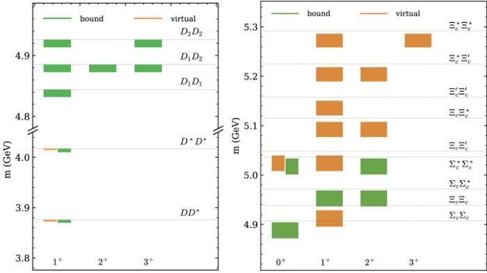
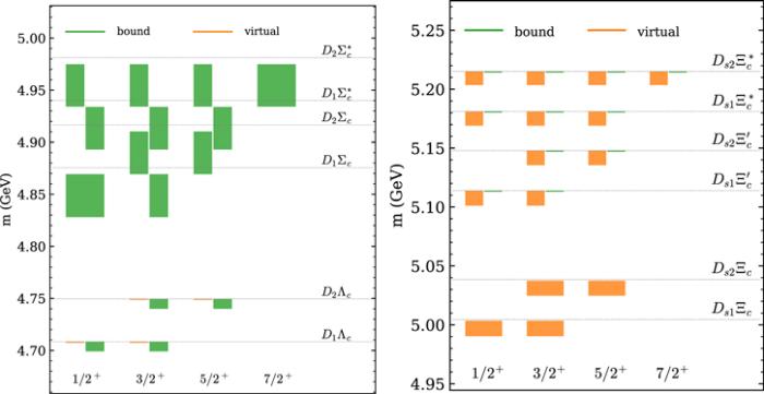
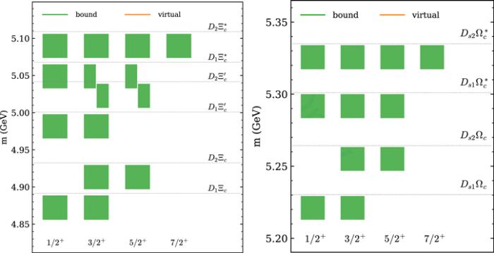
In tables 3, 4, 5 and 6, we list all the pole positions of the double-charm-hadron systems which have attractive interactions, corresponding to the masses of hadronic molecules (bound states on 1st RS or virtual states on 2nd RS). For better illustration, these states are also shown in figures 1, 2, 3, 4, 5 and 6 together with the corresponding thresholds. Considering the constant contact interactions saturated by the light vector meson exchange with the coupled-channel effects neglected, we obtain a spectrum of 124 hadronic molecules in total. At least the same number of molecules are expected to exist for each of the charm-bottom and bottom-bottom systems since it is easier to form a bound state with the same attraction strength due to the heavier reduced masses; there could be even more as if the ground state is deeply bound excited states might exist as well as illustrated in the Jülich meson-exchange model for hidden-bottom pentaquark-like hadronic molecules in [86].

Figure 1.

New window|Download| PPT slide
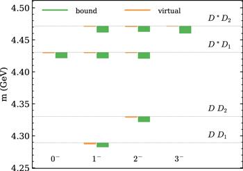
Figure 1.The spectrum of hadronic molecules consisting of a pair of charmed mesons or baryons with I = 0 and P = +. The colored rectangle, green for a bound state and orange for a virtual state, covers the range of the pole position for a given system with the cutoff Λ varying in the range of [0.5, 1.0] GeV. Thresholds are marked by dotted horizontal lines. The rectangle closest to, but below, the threshold corresponds to the hadronic molecule in that system. In some cases, e.g. DD^*, there are two rectangles for one system, with the upper edges exactly at the threshold. This corresponds to the situation that the pole moves from the second RS (left orange) to the first RS (right green) when Λ increases in the considered range. In some other cases where the pole positions of two systems overlap, small rectangles are used with the left (right) one for the system with the higher (lower) threshold.

Figure 2.

New window|Download| PPT slide
Figure 2.The spectrum of hadronic molecules consisting of a pair of charmed mesons with I = 0 and P = −. See the caption for figure 1.

Figure 3.

New window|Download| PPT slide
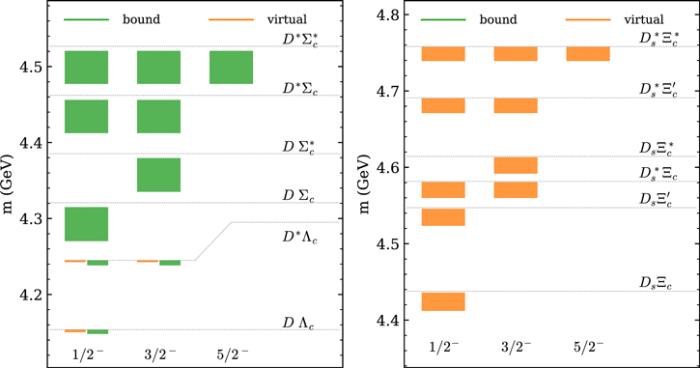
Figure 3.The spectrum of hadronic molecules consisting of a pair of charmed meson and charmed baryon with I = 1/2 and P = −. See the caption for figure 1. The right part of the dashed line for D^*Λ_c marks the real threshold while the left part is deformed to avoid being covered by the rectangle of DΣ_c system.

Figure 4.

New window|Download| PPT slide
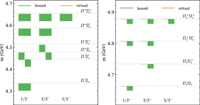
Figure 4.The spectrum of hadronic molecules consisting of a pair of charmed meson and charmed baryon with I = 0 and P = −. See the caption for figure 1.

Figure 5.

New window|Download| PPT slide
Figure 5.The spectrum of hadronic molecules consisting of a pair of charmed meson and charmed baryon with I = 1/2 and P = +. See the caption for figure 1.

Figure 6.

New window|Download| PPT slide
Figure 6.The spectrum of hadronic molecules consisting of a pair of charmed meson and charmed baryon with I = 0 and P = +. See the caption for figure 1.



Table 3.
Table 3.Pole positions of double-charm-hadron systems with I = 0 and P = +. E_th in the second column is the threshold in MeV. The results as given in the last columns corresponds to using the cutoff Λ = 0.5 (1.0) GeV for equation (17) used to determine the subtraction constant a(μ) in equation (15), respectively. In the last two columns, the first number in the parenthesis refers to the Riemann sheet (RS) where the pole is located while the second number means the distance between the pole position and the corresponding threshold, namely, E_B ≡ E_th − E_pole, in units of MeV.

System	Eth [MeV]	JP	(RS, EB [MeV])
			0.5 GeV	1.0 GeV
DD*	3876	1+	(2, 3.58)	(1, 5.96)
D*D*	4017	1+	(2, 2.68)	(1, 7.07)
D1D1	4844	1+	(2, 0.321)	(1, 12.2)
D1D2	4885	(1, 2, 3)+	(2, 0.277)	(1, 12.4)
D2D2	4926	(1, 3)+	(2, 0.237)	(1, 12.6)
ΣcΣc	4907	0+	(1, 2.72)	(1, 35.2)
ξcξc	4939	1+	(2, 43.4)	(2,10.1)
${{\rm{\Sigma }}}_{c}{{\rm{\Sigma }}}_{c}^{* }$	4972	(1, 2)+	(1, 2.79)	(1, 35.1)
${{\rm{\Sigma }}}_{c}^{* }{{\rm{\Sigma }}}_{c}^{* }$	5036	(0, 2)+	(1, 2.86)	(1, 35.1)
${{\rm{\Xi }}}_{c}{{\rm{\Xi }}}_{c}^{{\prime} }$	5048	(0, 1)+	(2, 40.1)	(2, 8.55)
${{\rm{\Xi }}}_{c}{{\rm{\Xi }}}_{c}^{* }$	5115	(1, 2)+	(2, 38.3)	(2, 7.73)
${{\rm{\Xi }}}_{c}^{{\prime} }{{\rm{\Xi }}}_{c}^{{\prime} }$	5158	1+	(2, 36.9)	(2, 7.14)
${{\rm{\Xi }}}_{c}^{* }{{\rm{\Xi }}}_{c}^{{\prime} }$	5225	(1, 2)+	(2, 35.2)	(2, 6.4)
${{\rm{\Xi }}}_{c}^{* }{{\rm{\Xi }}}_{c}^{* }$	5292	(1, 3)+	(2, 33.4)	(2, 5.7)
D1ξc	4891	${\left(\tfrac{1}{2},\tfrac{3}{2}\right)}^{+}$	(1, 2.78)	(1, 35.5)
D2ξc	4932	${\left(\tfrac{3}{2},\tfrac{5}{2}\right)}^{+}$	(1, 2.83)	(1, 35.5)
${D}_{1}{{\rm{\Xi }}}_{c}^{{\prime} }$	5001	${\left(\tfrac{1}{2},\tfrac{3}{2}\right)}^{+}$	(1, 2.89)	(1, 35.4)
${D}_{2}{{\rm{\Xi }}}_{c}^{{\prime} }$	5042	${\left(\tfrac{3}{2},\tfrac{5}{2}\right)}^{+}$	(1, 2.94)	(1, 35.4)
${D}_{1}{{\rm{\Xi }}}_{c}^{* }$	5068	${\left(\tfrac{1}{2},\tfrac{3}{2},\tfrac{5}{2}\right)}^{+}$	(1, 2.96)	(1, 35.3)
${D}_{2}{{\rm{\Xi }}}_{c}^{* }$	5109	${\left(\tfrac{1}{2},\tfrac{3}{2},\tfrac{5}{2},\tfrac{7}{2}\right)}^{+}$	(1, 3.0)	(1, 35.3)
Ds1ωc	5230	${\left(\tfrac{1}{2},\tfrac{3}{2}\right)}^{+}$	(1, 0.0298)	(1, 17.4)
Ds2ωc	5264	${\left(\tfrac{3}{2},\tfrac{5}{2}\right)}^{+}$	(1,0.039)	(1, 17.5)
${D}_{s1}{{\rm{\Omega }}}_{c}^{* }$	5301	${\left(\tfrac{1}{2},\tfrac{3}{2},\tfrac{5}{2}\right)}^{+}$	(1, 0.0474)	(1, 17.6)
${D}_{s2}{{\rm{\Omega }}}_{c}^{* }$	5335	${\left(\tfrac{1}{2},\tfrac{3}{2},\tfrac{5}{2},\tfrac{7}{2}\right)}^{+}$	(1, 0.0588)	(1, 17.7)

New window|CSV


Table 4.
Table 4.Pole positions of double-charm-hadron systems with I = 0 and P = −. See the caption for table 3.

System	Eth [MeV]	JP	(RS, EB [MeV])
			0.5 GeV	1.0 GeV
DD1	4289	1−	(2, 2.48)	(1, 6.94)
DD2	4330	2−	(2, 1.65)	(1, 8.69)
D*D1	4431	(0, 1, 2)−	(2, 1.35)	(1, 9.12)
D*D2	4472	(1, 2, 3)−	(2, 1.0)	(1, 10.1)
D ξc	4337	${\tfrac{1}{2}}^{-}$	(1, 1.92)	(1, 35.3)
$D\ {{\rm{\Xi }}}_{c}^{{\prime} }$	4446	${\tfrac{1}{2}}^{-}$	(1, 2.04)	(1, 35.4)
D*ξc	4478	${\left(\tfrac{1}{2},\tfrac{3}{2}\right)}^{-}$	(1, 2.19)	(1, 35.5)
$D\ {{\rm{\Xi }}}_{c}^{* }$	4513	${\tfrac{3}{2}}^{-}$	(1,2.11)	(1, 35.4)
${D}^{* }{{\rm{\Xi }}}_{c}^{{\prime} }$	4587	${\left(\tfrac{1}{2},\tfrac{3}{2}\right)}^{-}$	(1, 2.31)	(1, 35.5)
${D}^{* }{{\rm{\Xi }}}_{c}^{* }$	4655	${\left(\tfrac{1}{2},\tfrac{3}{2},\tfrac{5}{2}\right)}^{-}$	(1, 2.38)	(1, 35.5)
Dsωc	4664	${\tfrac{1}{2}}^{-}$	(2, 0.168)	(1, 14.3)
${D}_{s}{{\rm{\Omega }}}_{c}^{* }$	4734	${\tfrac{3}{2}}^{-}$	(2, 0.129)	(1, 14.6)
${D}_{s}^{* }{{\rm{\Omega }}}_{c}^{{\prime} }$	4807	${\left(\tfrac{1}{2},\tfrac{3}{2}\right)}^{-}$	(2, 0.0507)	(1, 15.3)
${D}_{s}^{* }{{\rm{\Omega }}}_{c}^{* }$	4878	${\left(\tfrac{1}{2},\tfrac{3}{2},\tfrac{5}{2}\right)}^{-}$	(2, 0.0308)	(1, 15.6)

New window|CSV


Table 5.
Table 5.Pole positions of double-charm-hadron systems with I = 1/2 and P = −. See the caption for table 3.

System	Eth [MeV]	JP	(RS, EB [MeV])
			0.5 GeV	1.0 GeV
D Λc	4154	${\tfrac{1}{2}}^{-}$	(2, 3.44)	(1, 5.62)
D*Λc	4295	${\left(\tfrac{1}{2},\tfrac{3}{2}\right)}^{-}$	(2, 2.53)	(1, 6.73)
D Σc	4321	${\tfrac{1}{2}}^{-}$	(1, 5.81)	(1, 50.5)
$D\ {{\rm{\Sigma }}}_{c}^{* }$	4385	${\tfrac{3}{2}}^{-}$	(1, 5.85)	(1, 50.2)
D*Σc	4462	${\left(\tfrac{1}{2},\tfrac{3}{2}\right)}^{-}$	(1, 5.97)	(1, 49.7)
${D}^{* }{{\rm{\Sigma }}}_{c}^{* }$	4527	${\left(\tfrac{1}{2},\tfrac{3}{2},\tfrac{5}{2}\right)}^{-}$	(1,6.01)	(1, 49.5)
Dsξc	4438	${\tfrac{1}{2}}^{-}$	(2, 25.7)	(2, 1.76)
${D}_{s}{{\rm{\Xi }}}_{c}^{{\prime} }$	4547	${\tfrac{1}{2}}^{-}$	(2, 23.7)	(2, 1.29)
${D}_{s}^{* }{{\rm{\Xi }}}_{c}$	4582	${\left(\tfrac{1}{2},\tfrac{3}{2}\right)}^{-}$	(2, 21.8)	(2, 0.882)
${D}_{s}{{\rm{\Xi }}}_{c}^{* }$	4614	${\tfrac{3}{2}}^{-}$	(2, 22.6)	(2, 1.05)
${D}_{s}^{* }{{\rm{\Xi }}}_{c}^{{\prime} }$	4691	${\left(\tfrac{1}{2},\tfrac{3}{2}\right)}^{-}$	(2, 20.0)	(2, 0.564)
${D}_{s}^{* }{{\rm{\Xi }}}_{c}^{* }$	4758	${\left(\tfrac{1}{2},\tfrac{3}{2},\tfrac{5}{2}\right)}^{-}$	(2, 19.0)	(2, 0.416)

New window|CSV


Table 6.
Table 6.Pole positions of double-charm-hadron systems with I = 1/2 and P = +. See the caption for table 3.

System	Eth [MeV]	JP	(RS, EB [MeV])
			0.5 GeV	1.0 GeV
D1Λc	4708	${\left(\tfrac{1}{2},\tfrac{3}{2}\right)}^{+}$	(2, 1.04)	(1, 9.31)
D2Λc	4750	${\left(\tfrac{3}{2},\tfrac{5}{2}\right)}^{+}$	(2, 0.95)	(1, 9.51)
D1Σc	4876	${\left(\tfrac{1}{2},\tfrac{3}{2}\right)}^{+}$	(1, 6.25)	(1, 47.5)
D2Σc	4917	${\left(\tfrac{3}{2},\tfrac{5}{2}\right)}^{+}$	(1, 6.27)	(1, 47.3)
${D}_{1}{{\rm{\Sigma }}}_{c}^{* }$	4940	${\left(\tfrac{1}{2},\tfrac{3}{2},\tfrac{5}{2}\right)}^{+}$	(1,6.28)	(1, 47.2)
${D}_{2}{{\rm{\Sigma }}}_{c}^{* }$	4981	${\left(\tfrac{1}{2},\tfrac{3}{2},\tfrac{5}{2},\tfrac{7}{2}\right)}^{+}$	(1, 6.29)	(1, 47.0)
Ds1ξc	5005	${\left(\tfrac{1}{2},\tfrac{3}{2}\right)}^{+}$	(2, 14.2)	(2, 0.00911)
Ds2ξc	5039	${\left(\tfrac{3}{2},\tfrac{5}{2}\right)}^{+}$	(2, 13.8)	(2, 0.00176)
${D}_{s1}{{\rm{\Xi }}}_{c}^{{\prime} }$	5114	${\left(\tfrac{1}{2},\tfrac{3}{2}\right)}^{+}$	(2, 12.8)	(1, 0.00636)
${D}_{s2}{{\rm{\Xi }}}_{c}^{{\prime} }$	5148	${\left(\tfrac{3}{2},\tfrac{5}{2}\right)}^{+}$	(2, 12.4)	(1, 0.0175)
${D}_{s1}{{\rm{\Xi }}}_{c}^{* }$	5181	${\left(\tfrac{1}{2},\tfrac{3}{2},\tfrac{5}{2}\right)}^{+}$	(2, 12.0)	(1, 0.0319)
${D}_{s2}{{\rm{\Xi }}}_{c}^{* }$	5215	${\left(\tfrac{1}{2},\tfrac{3}{2},\tfrac{5}{2},\tfrac{7}{2}\right)}^{+}$	(2, 11.6)	(1, 0.0532)

New window|CSV

Besides the predicted molecular states mentioned above, where only ω, ρ and φ exchanges are considered, we need pay some extra attentions to the K^* exchange, which is absent in the heavy–antiheavy systems due to the sizeable symmetry breaking between s quark and u/d quark. In most cases, K^* exchange, if allowed, will contribute a repulsive potential, see table 7, unless two channels are close enough and can be linearly combined to an isospin-like (called U/V-spin in [87]) eigenstates. Explicitly, the thresholds of ${{DD}}_{s}^{* }$ and D^*D_s are close enough and they may form two U/V-spin eigenstates,(18)$\begin{eqnarray}U/V=\pm :{{DD}}_{s}^{* }\pm {D}^{* }{D}_{s}.\end{eqnarray}$The potentials of K^* exchange are repulsive and attractive, respectively, the strength of which can be also described by equation (13) with ∣F∣ = 1 and ${m}_{\mathrm{ex}}={m}_{{K}^{* }}$. Therefore, we expect a near threshold virtual or bound states in the U/V = − 1 systems of ${{DD}}_{s}^{* }$. Some other similar systems, such as ${{\rm{\Sigma }}}_{c}{{\rm{\Xi }}}_{c}^{* }$ and ${{\rm{\Sigma }}}_{c}^{* }{{\rm{\Xi }}}_{c}$, the thresholds are not that close and more efforts should be paid to the coupled channel efforts, which is beyond the scope of this work.

4. Discussions of selected systems

4.1. Heavy meson–meson molecules versus doubly heavy tetraquarks

From table 7, one sees that the attraction strength for the isoscalar D^(*)D^* is half of that for the isoscalar C = + ${D}^{(* )}{\bar{D}}^{* }$ pairs.⁹(9 For the isoscalar systems, ${V}_{{D}^{(* )}{D}^{* }}=\tfrac{3}{2}{V}_{\rho }-\tfrac{1}{2}{V}_{\omega }$, which is about half of ${V}_{{D}^{(* )}{\bar{D}}^{* }}=\tfrac{3}{2}{V}_{\rho }+\tfrac{1}{2}{V}_{\omega }$ considering V_ρ ≈ V_ω, where V_ρ and V_ω are the potentials due to the exchange of ρ and ω, respectively.)Thus, for the X(3872) as a $D{\bar{D}}^{* }$ bound state with J^PC = 1⁺⁺,¹⁰(10 Notice that the narrow structure X(4014) reported recently by Belle [88] is an excellent candidate for the 2⁺⁺ ${D}^{* }{\bar{D}}^{* }$ molecule [89, 90, 84, 85, 91, 92, 32], and its mass (4014.4 ± 4.1 ± 0.5) MeV and width (6 ± 16 ± 6) MeV nicely agree with the predictions in [91]. The $D\bar{D}$ bound state obtained in the same way [32] (for early predictions, see [93–96, 84, 97]) also receives support from a recent lattice QCD calculation [98].) the D^(*)D^* system would be less. From figure 2 we see indeed that the isoscalar D^(*)D^* systems are at the edge of forming bound states. While for the isovector ones, the potential from ρ and ω exchange is repulsive and thus no molecules are expected. The situations for D^(*)D_(1,2) and D_(1,2)D_(1,2) systems are all similar.

The ${T}_{{cc}}^{+}$ state was recently observed in the invariant mass distribution of D⁰D⁰π⁺ by LHCb [39, 40]. The pole from an analysis using a unitarized Breit–Wigner parameterization, considering the momentum-dependent width of the D^* from its decays, is located in the complex energy plane at(19)$\begin{eqnarray}-360\pm {40}_{-0}^{+4}-\mathrm{i}(24\pm {2}_{-7}^{+0})\,\mathrm{keV},\end{eqnarray}$with the real part defined as the energy relative to the D⁰D^*+ threshold [40].¹¹(11 A simple Breit–Wigner parametrization of the peak convolved with energy resolution leads to a width of (410 ± 165) keV [39]. Note that the ${T}_{{cc}}^{+}$ is very close to the D⁰D^*+ threshold, and thus the Flatté parameterization is more proper than the Breit-Wigner one; the former leads to a asymmetric line shape automatically while the latter does not. It is also worthwhile to notice that the width of a Flatté line shape can be much smaller than that of the Breit–Wigner one when convolved with the energy resolution, as nicely illustrated in the careful analysis of the X(3872) line shape by the LHCb Collaboration [99].) This new state is a good candidate of the isoscalar DD^* molecule, in agreement with our result. Before this experiment signal, lots of predictions of such doubly charmed tetraquark states, being either hadronic molecules [100–105] or compact tetraquark states [105–135], have been made with various methods.

4.1.1. Heavy meson–meson molecules

The doubly heavy tetraquark states in molecular configurations were widely investigated in the literature [89, 100–105, 136–165] where predictions of many doubly heavy tetraquark states including the T_cc mentioned above as well as other systems were made.

The interaction between a pair of heavy mesons was estimated using the Born–Oppenheimer approximation in the MIT bag model in [106]. The I(J^P) = 0(1⁺) di-meson $T({bb}\bar{q}\bar{q})$ was found to be a bound state about 70 MeV below the BB^* threshold while the situations of $T({bc}\bar{q}\bar{q})$ and $T({cc}\bar{q}\bar{q})$ were uncertain.

By solving the double-charm tetraquark system with two realistic potential models, it was found in [100] that the ground state tetraquark state has a configuration of DD^* molecule. In the constituent quark model, it was also found that the di-meson configurations of ${QQ}\bar{q}\bar{q}$ can be bound [105].

In [162], the B^(*)B^(*) scattering amplitude was explored in the constituent interchange model and the I(J^P) = 0(1⁺) BB^* and B^*B^* bound states together with virtual states with some other quantum numbers were found.

In [137], it was found that the long-range potential from one-pion exchange may be attractive enough to bind the BB^* system but insufficient for the DD^* system to bind, which has a smaller reduced mass. The existence of DD^* was also disfavored by the one pion exchange in [89]. While the one-boson exchange model predicts that the isoscalar DD^* system can form an S-wave bound state with a binding energy of 62.3 MeV (depending on the cutoff) with the π, ρ and ω exchanges [101], 3 ∼ 40 MeV with the π, ρ and ω exchanges [104], 0.47 ∼ 43 MeV (depending on the cutoff) after including the π, Σ, ρ and ω exchanges and coupled channel effects [102] or ${3}_{-\,4}^{+15}$ MeV without coupled channels but with the cutoff fixed by producing the correct binding energy of X(3872) [103]. Besides, some other doubly heavy molecules including ${D}_{(s)}^{(* )}{D}_{(s)}^{(* )}$, ${\bar{B}}_{(s)}^{* }{\bar{B}}_{(s)}^{(* )}$ and ${D}^{(* )}{\bar{B}}^{(* )}$ with different quantum numbers are predicted in these works as well as in [165]. In [144], the potential between DD^* from the one-pion exchange supplemented by the contact term and the exchange of two pions was investigated in a chiral effective field theory, and an isovector state was found to be bound while the scalar one was not.

With the potential from a chiral constituent quark model, the LippmannSchwinger equation was solved for the DD-DD^*-D^*D^* coupled channels in [142] and a stable doubly charmed meson with I(J^P) = 0(1⁺) was predicted. In [145], the similar strategy yielded isoscalar 0⁺ and 1⁺ ${bc}\bar{q}\bar{q}$ bound states, which are stable against strong interaction, but the isovector systems were found unbound.

We can notice that the results from these works, as well as those obtained here, do not all agree with each other. There are at least two possible reasons: the form of the potential, in particular the treatment of the short-distance part, is different; the parameter values are different. In the spirit of effective field theory, different treatments of the short-distance potential correspond to taking different values for the contact terms In any case, most of the literature tends to agree that it is easier for the isoscalar DD^*/BB^* to bind than the isovector combinations, as is the conclusion in our paper as well. Our model assumes the short-distance contact terms are saturated by the light-vector-meson exchange, and the long- or mid-range attractive potential from the π or Σ exchanges and the coupled channel effects may change the hadronic molecule spectrum quantitatively to some extent.

There are also lattice calculations of the potential between a pair of heavy mesons [136, 138, 139, 148, 149]. The DD^(*) interactions were calculated on lattice [150] and it was found that the potentials of the isovector systems are repulsive while those of the isoscalar systems are attractive, qualitatively in line with the contact interactions from the vector meson exchange reported here (see table 7). The isoscalar B^(*)B^(*) interaction from lattice calculations [147, 151–156] in the static b quark limit is attractive in the short range while for the isovector one, the attraction is weaker. It was found plausible for $\bar{b}\bar{b}{qq}$ di-mesons to be stable under strong interactions [146]. In [153–157], the Schrödinger equation with the obtained potential yields results that the I(J^P) = 0(1⁺) $\bar{b}\bar{b}{qq}$ system has an attractive potential between two B^(*) mesons strong enough to form bound states but not strong enough in the isovector case. A recent analysis on lattice [166] shows that the meson–meson component in the I(J^P) = 0(1⁺) $\bar{b}\bar{b}{ud}$ state has a fraction around 60%.

4.1.2. Compact tetraquark states

Besides the molecular assignment, many works have investigated the compact doubly heavy tetraquarks via various methods, including quark potential models [107–109, 167–179], quark models with heavy quark symmetries [110, 121, 120], QCD sum rules [112, 122, 180–189] and lattice QCD [190–195].

In the quark potential models, it was found that the $\bar{Q}\bar{Q}{qq}$ is possible to be bound below the two-meson threshold for certain potentials [167–170] but no bound states can be found if all quarks have the same mass, which was confirmed recently in a four-body calculation [173]. It was also found [174] that although the possible configurations of tetraquarks proliferate, only five of the candidates are stable, namely, ${cc}\bar{q}\bar{q}$ with J^P(L, S, I) = 1⁺(0, 1, 0) and ${bb}\bar{q}\bar{q}$ with J^P(L, S, I) = 1⁺(0, 1, 0), 3⁻(1, 2, 1), 0⁺(0, 0, 0) and 1⁻(1, 0, 0), where L and S refer to the orbital angular momentum and total spin of the two mesons that couple to the tetraquark, among which the last one has a molecular nature. The doubly charmed system was also confirmed to be bound in [196] using different potential models while in [197] only one doubly-bottomed system with I(J^P) = 0(1⁺) was found to be located below the threshold of the corresponding meson pair. With an adequate treatment of the four-body dynamics in the quark model picture of tetraquark states, it was found in [198] that the I(J^P) = 0(1⁺) ${cc}\bar{u}\bar{d}$ system is at the edge of binding while the doubly-bottomed system is easier to be bound. On the other hand, the analysis within the chiral SU(3) quark model [199] or the relativistic quark model [113] found that the I(J^P) = 0(1⁺) ${cc}\bar{u}\bar{d}$ state is not bound but above the thresholds for decays into open charm mesons. In [164], two bound states of I(J^P) = 0(1⁺) ${bb}\bar{u}\bar{d}$ were found in a constituent quark model, one deeply bound compact tetraquark and one BB^* molecule.

In [200], the masses of tetraquark states were obtained model-independently with known hadron masses as input and it was found that four-quark states containing two identical heavy quarks have a good probability of being stable against strong decay. In [120], the ground states of hadrons are described by the quark model and therein the mass of the predicted J^P = 1⁺ ${cc}\bar{u}\bar{d}$ state reads (3882 ± 12) MeV using the measured ${{\rm{\Xi }}}_{{cc}}^{++}$ mass [201] as input, which nicely covers the LHCb result. [120] also predicts a 1⁺ ${bb}\bar{u}\bar{d}$ state to be at (10389 ± 12) MeV, which is well below the BB^* threshold and thus stable under strong and electromagnetic interactions.

By implementing the heavy antiquark-diquark symmetry [202], the mass of doubly-heavy tetraquark states may be predicted using the relation(20)$\begin{eqnarray}m({QQ}\bar{q}\bar{q})-m({QQq})\approx m({Qqq})-m(Q\bar{q}),\end{eqnarray}$the essence of which can be traced back to [203, 204]. For instance, after the double-charm baryon ${{\rm{\Xi }}}_{{cc}}^{++}$ was observed [201], the lightest double-bottom tetraquark state was predicted in [121] to be at 10 482 MeV, which is below the BB^* threshold and stable under strong and electromagnetic interactions, with J^P = 1⁺, using the doubly-bottom baryon masses in [205] as input. The mass of ${cc}\bar{u}\bar{d}$ was determined in this way to be 3845 or 3905 MeV [110], 3978 MeV [121], (3947 ± 11) MeV [131], 3900 MeV [117] and 3929 MeV [133], see also the discussion in [206]. The spectrum of some other doubly-heavy tetraquark states were also obtained in these works, including stable ${bb}\bar{q}\bar{q}$ tetraquark states. Note that different from the case of doubly-heavy baryons, where the heavy diquark must be in a color anti-triplet, the two heavy quarks inside a doubly-heavy tetraquark can be in either a color anti-triplet or a color sextet. The approximate heavy antiquark-diquark symmetry is applicable only when the color sextet component of the diquark can be neglected and when the two heavy quarks are close to each other so that they acts as a pointlike color-antitriplet source just like a heavy antiquark. Thus, it cannot be applied to relate the heavy–heavy molecular systems to singly-heavy baryons. Tetraquarks with the two charm quarks as a compact diquark may exist in addition to the molecular states. The mixing of these two configurations will make the spectrum more complicated.

The spectrum of ${QQ}\bar{q}\bar{q}$ tetraquark states are explored via the method of QCD sum rules in [112, 122, 180–189]. In [181] it was argued that the molecular current of DD^* yields a similar mass with that of the $D{\bar{D}}^{* }+c.c.$ molecule and thus the result will perfectly match ${T}_{{cc}}^{+}$ mass measured by LHCb if X(3872) is a $D{\bar{D}}^{* }+c.c.$ molecule. The mass of the ${cc}\bar{u}\bar{d}$ ground state with J^P = 1⁺ was determined to be (3.90 ± 0.09) GeV in [122, 183], which is also consistent with LHCb result. While in other works, it was found that usually the J^P = 1⁺ ${bb}\bar{u}\bar{d}$ state lies below the threshold of BB^* [112, 185, 186] while the charmed one is above the corresponding DD^* threshold [112, 180, 186].

The explorations of doubly-heavy compact tetraquark states on lattice can be seen in, e.g. [124, 126, 190–195, 207]. Deeply bound tetraquark states, ${ud}\bar{b}\bar{b}$, ${qs}\bar{b}\bar{b}$ and ${ud}\bar{b}\bar{c}$ with J^P = 1⁺ are predicted in [191, 194], which are 189 ± 10, 98 ± 7 and 15 ∼ 61 MeV below the corresponding free two-meson thresholds, respectively. [126] obtained similar results for the above systems and predicted another three bound states of ${uc}\bar{b}\bar{b}$, ${ud}\bar{c}\bar{c}$ and ${us}\bar{c}\bar{c}$ located just below the corresponding free two-meson thresholds, and the masses of the double-charm states are in agreement with those obtained in [124, 192]. In [195], the tetraquark operators for ${bb}\bar{u}\bar{d}$ are constructed in both diquark-antidiquark ($[{bb}][\bar{u}\bar{d}]$) and molecular ($[b\bar{u}][b\bar{d}]$) configurations and two states were found on lattice, a compact tetraquark located at 189 ± 18 MeV below BB^* threshold and a molecular one 17 ± 14 MeV above the same threshold.

4.2. Heavy meson-baryon molecules versus doubly heavy baryons

Different from the meson–meson case, from table 7 we can see that double-charm meson-baryon systems are more attractive or less repulsive than the hidden-charm ones. Specifically, the ${D}^{(* )}{{\rm{\Sigma }}}_{c}^{(* )}$ systems with isospin-1/2 are more attractive than the isospin-1/2 ${\bar{D}}^{(* )}{{\rm{\Sigma }}}_{c}^{(* )}$ systems while the latter are widely believed to be able to form bound states with experimental candidates, namely, the famous P_c states [15]. Therefore, it is natural that more deeply bound states of ${D}^{(* )}{{\rm{\Sigma }}}_{c}^{(* )}$ exist, see figure 3. Similar conclusions can be drawn for ${D}_{\mathrm{1,2}}{{\rm{\Sigma }}}_{c}^{(* )}$ systems, as shown in figure 5, since they have the same form of leading order interactions. Other systems including ${D}^{(* )}{{\rm{\Xi }}}_{c}^{(^{\prime} * )}$, ${D}_{\mathrm{1,2}}{{\rm{\Xi }}}_{c}^{(^{\prime} * )}$, ${D}_{s}^{(* )}{{\rm{\Omega }}}_{c}^{(* )}$ and ${D}_{s1,s2}{{\rm{\Omega }}}_{c}^{(* )}$ are also predicted to be bound easily, the spectra of which are shown in figures 4 and 6.

Similarly with the coupled channel analysis used in the pioneering works [208, 81] of pentaquark states where the P_c states were successfully predicted, [209] extended such a study to the double-charm systems and some deeply bound states of ${D}^{(* )}{{\rm{\Sigma }}}_{c}^{(* )}$ with binding energies of ${ \mathcal O }$(100 MeV) were found. It was extended further to the charm-bottom system and double-bottom systems in [210, 211], and more deeply bound states of ${D}^{(* )}{{\rm{\Sigma }}}_{b}^{(* )}$ and ${\bar{B}}^{(* )}{{\rm{\Sigma }}}_{c}^{(* )}$ with binding energies of ${ \mathcal O }$(300MeV) and ${\bar{B}}^{(* )}{{\rm{\Sigma }}}_{b}^{(* )}$ with binding energies of ${ \mathcal O }$(400 MeV) were obtained. There it was also found that there are poles located about 100 MeV below the Λ_bD, ${{\rm{\Lambda }}}_{c}\bar{B}$ and ${{\rm{\Lambda }}}_{b}\bar{B}$ thresholds, respectively. Such conclusions are qualitatively consistent with our results that ${D}^{(* )}{{\rm{\Sigma }}}_{c}^{(* )}$ and ${D}^{(* )}{{\rm{\Xi }}}_{c}^{(* )}$ are attractive and the former is stronger. The meson-baryon transitions between the coupled channels J/ψN-${{\rm{\Lambda }}}_{c}{\bar{D}}^{(* )}$-${{\rm{\Sigma }}}_{c}^{(* )}{\bar{D}}^{(* )}$ were explored in [212] and it was found that a doubly-charmed state, ${{\rm{\Xi }}}_{{cc}}^{* }(4380)$, exists with almost the same mass as P_c(4380). An S-wave scattering of ground state doubly-charmed baryons with the light pseudoscalar mesons were first investigated in [75] and then in [213] by means of unitarized chiral effective theory and several doubly charmed baryon resonances were predicted. The spectrum was modified by including the effects of the P-wave excitation inside the charm diquark in [214].

The interaction between DΛ_c or $\bar{B}{{\rm{\Lambda }}}_{b}$ from two-pion exchange are investigated in [215] and it was claimed that a $\bar{B}{{\rm{\Lambda }}}_{b}$ bound state from such an interaction is possible. In [216], the DΛ_c/b, $\bar{B}{{\rm{\Lambda }}}_{c/b}$ systems were found possible to be bound by the Σ/ω exchange interaction. Systematic studies on the ${{\rm{\Sigma }}}_{c}^{(* )}{D}^{(* )}$ interactions within the framework of chiral effective field theory [217] or one boson exchange [104] were performed, and the I = 1/2 systems may form bound states with binding energies of about several or dozens MeV, consistent with the results obtained here, see table 5. Therein, deeper bound states of the ${{\rm{\Sigma }}}_{c}^{(* )}{\bar{B}}^{(* )},{{\rm{\Sigma }}}_{b}^{(* )}{D}^{(* )}$ and ${{\rm{\Sigma }}}_{b}^{(* )}{\bar{B}}^{(* )}$ systems were also predicted to exist due to the larger reduced masses, as expected.

The doubly-heavy pentaquark states with compact configurations were explored within the color-magnetic interaction model [218], non-relativistic constituent quark model [219] and QCD sum rules [220, 221] where some narrow exotic pentaquark states were predicted, constituent quark model [222] where one strong-interaction stable state, ${ccud}\bar{s}$ was predicted.

From table 5 and figure 3, one sees that the lightest double-charm meson-baryon molecule is the one in the DΛ_c system. The state has a mass large enough for it to decay into ξ_ccπ and could be broad. So are the other similar states.

4.3. Heavy di-baryons

For heavy di-baryons, the leading order interaction from the vector meson exchange leads to evident binding only for the ${{\rm{\Sigma }}}_{c}^{(* )}{{\rm{\Sigma }}}_{c}^{(* )}$ systems, see table 3 and figure 1. The attractions for the ξ_cξ_c related systems are too weak and only remote virtual poles are found, which are not robust somehow and can get sizeably modified by the omitted momentum-dependent terms

In our simple model the leading order interaction for the Λ_cΛ_c system is repulsive and thus it cannot be bound. Within various models, it was found that the Λ_cΛ_c system can not be bound by itself [223–228] but [224–226, 229] showed that the coupling to the strongly attractive ${{\rm{\Sigma }}}_{c}^{(* )}{{\rm{\Sigma }}}_{c}^{(* )}$ system may lead to a states below Λ_cΛ_c threshold . In an analysis with QCD sum rules [230], the states with the same quark components as Λ_cΛ_c were found all above the Λ_cΛ_c threshold. In [231, 232, 216], on the contrary, the single channel Λ_cΛ_c can be bound by itself; however, [232] warns that a more thorough theoretical exploration is needed to determine whether the Λ_cΛ_c system really binds.

Some other doubly-heavy di-baryon systems were also explored. Several realistic phenomenological nucleon-nucleon interaction models are employed in [233]. It was found there that the ${{\rm{\Xi }}}_{c}^{(^{\prime} )}{{\rm{\Xi }}}_{c}^{(^{\prime} )}$ and Σ_cΣ_c systems can be bound in some models. From one-boson exchange with coupled channel effects included, [223, 234] found that ${{\rm{\Xi }}}_{c}^{(^{\prime} * )}{{\rm{\Xi }}}_{c}^{(^{\prime} * )}$ and ${{\rm{\Omega }}}_{c}^{(* )}{{\rm{\Omega }}}_{c}^{(* )}$ may be loosely bound while the isoscalar ${{\rm{\Sigma }}}_{c}^{(* )}{{\rm{\Sigma }}}_{c}^{(* )}$ systems can be deeply bound. Similar conclusion was obtained in [225] within the framework of quark delocalization color screening model that the ${{\rm{\Sigma }}}_{c}^{(* )}{{\rm{\Sigma }}}_{c}^{(* )}$ single-channel system can be deeply bound. In [228], the potential of Σ_cΣ_c was derived from a constituent quark model and a bound state with I(J^P) = 0(0⁺) was obtained with a binding energy about 6.2 MeV. The long-range pion exchange force is strong enough to form molecules of ${\left[{{\rm{\Sigma }}}_{Q}{{\rm{\Xi }}}_{Q}^{{\prime} }\right]}_{J=1}^{I=1/2}$, ${\left[{{\rm{\Sigma }}}_{Q}{{\rm{\Lambda }}}_{Q}\right]}_{J=1}^{I=1}(Q\,=b,c)$, ${\left[{{\rm{\Sigma }}}_{b}{{\rm{\Xi }}}_{b}^{{\prime} }\right]}_{J=1}^{I=3/2}$ and ${\left[{{\rm{\Xi }}}_{b}{{\rm{\Xi }}}_{b}^{{\prime} }\right]}_{J=1}^{I=0}$ where the S-D mixing is necessary [229]. In [232], the ${{\rm{\Sigma }}}_{Q}^{(* )}{{\rm{\Sigma }}}_{Q}^{(* )}$ were claimed to be good candidates of bound states from the one-pion and vector meson exchanges while it concludes that a more thorough analysis is necessary to determine whether there is a binding for the ${{\rm{\Lambda }}}_{Q}{{\rm{\Sigma }}}_{Q}^{(* )}$.

The di-baryon systems with two heavy quarks were investigated in [235] with a simple quark model but no bound or metastable state was found.

5. Summary

In this work we have obtained an overall spectrum of hadronic molecules composed of a pair of charmed hadrons, including all the S-wave singly-charmed mesons and baryons as well as the s_ℓ = 1/2 P-wave charmed mesons. The interaction is assumed to be dominated by the light vector meson exchange and approximated by constants at leading order, which are derived systematically from the couplings that satisfy HQSS and SU(3) flavor symmetry.

One should keep in mind that the spectrum predicted here should be regarded as the leading approximation of the spectrum for heavy–heavy molecular states, which gives only a general overall feature of the heavy–heavy hadronic molecular spectrum. The numerical results can receive large quantitative corrections due to the limitations of our treatments, which we discuss qualitatively in the following.• We have only considered the leading interactions described by constant contact terms The momentum dependent terms (including both spin-dependent and spin-independent contributions) may change the spectrum we obtained visibly, especially for the systems where the poles are far away from the corresponding thresholds. The spin-dependent terms will also lift the degeneracy of the same system with different total spins.
• The coupled channel effects have been neglected. In some cases the coupled-channel effects may play an important role in the formation of near threshold states. However, it is common and natural that the near-threshold pole found in a coupled-channel system dominantly couples to a single channel, see, e.g. the ${D}_{s0}^{* }(2317)$, which is dynamically generated in the DK and D_sη system but couples dominantly to DK [236, 237, 94], and the ξ_cc(4083) state with J^P = 1/2⁻, which is dynamically generated in the Σ_cD and ${{\rm{\Xi }}}_{c}^{{\prime} }{D}_{s}$ system but couples dominantly to Σ_cD [209].¹²(12 The Σ_cD bound state obtained in this work has a mass around 4.3 GeV, much closer to the threshold; see table 5 and figure 3.)
• The hadronic molecules shown in figures 3–6 can couple to normal double-charm baryons as well as channels with a double-charm baryon and a light meson. It is expected that each of these two types of systems also forms a spectrum. The physical spectrum of double-charm baryons should incorporate the mixing among all the three spectra. Coupled channels including both the charm-baryon–charm-meson channels and light-meson–double-charm-baryon channels have been considered in, e.g. [209] for the ξ_cc type molecular states. Mixing of light-meson–double-charm-baryon molecular states with the normal double-charm baryons with a P-wave excitation inside the charm diquark has been considered in [214]. Yet, a model considering all the three kinds of channels does not exist so far.
• The exchange of other particles, such as the light scalar mesons, charmed mesons and charmonia, are not considered, the effect of which can be partly covered by varying the cutoff. In addition, the interactions considered here are of leading order in the 1/N_c expansion, where N_c is the number of colors, i.e. the Okubo–Zweig–Iizuka violating interactions have been neglected. Such contributions will also lift the degeneracy of the same system with different total spins.


Therefore, although we expect the spectrum given here should present an overall pattern of the hadronic molecules formed by a pair of charmed mesons and/or baryons, specific systems may quantitatively differ from the predictions here due to the limitations of our treatments.

In total we obtained 124 double-charm hadronic molecules and we summarize the main feature of this spectrum in the following.1. Unlike the isovector D^*D^(*) systems that are repulsive, the isoscalar ones have attractive interaction from the light vector meson exchange and the total potential makes the systems at the edge of forming near-threshold molecules. With a reasonable cutoff regularizing the loop integral, the binding energy of the I(J^P) = 0(1⁺) DD^* system is consistent with the double charm tetraquark ${T}_{{cc}}^{+}$ in LHCb observation. If the hadronic molecule structure of the ${T}_{{cc}}^{+}$ is confirmed, which is rather natural given the closeness to the DD^* threshold, many other similar states with I = 0 including D^*D^*, D^(*)D_1,2, D_1,2D_1,2 can also exist.
2. Given that the famous P_c states are hadronic molecules of ${\bar{D}}^{(* )}{{\rm{\Sigma }}}_{c}^{(* )}$, it is natural to expect the existence of double-charm ${D}^{(* )}{{\rm{\Sigma }}}_{c}^{(* )}$ and ${D}_{\mathrm{1,2}}{{\rm{\Sigma }}}_{c}^{(* )}$ states with I = 1/2 because the attraction from the light vector meson exchange for the latter is stronger than that for the former. Similar conclusions can be made for the ${D}^{(* )}{{\rm{\Xi }}}_{c}^{(^{\prime} * )}$ and ${D}_{\mathrm{1,2}}{{\rm{\Xi }}}_{c}^{(^{\prime} * )}$ channels, especially when the P_cs states are established experimentally. The hadronic molecules in other systems including D^(*)Λ_c, D_1,2Λ_c, ${D}_{s}^{(* )}{{\rm{\Xi }}}_{c}^{(^{\prime} * )}$, ${D}_{s\mathrm{1,2}}{{\rm{\Xi }}}_{c}^{(^{\prime} * )}$ ${D}_{s}^{(* )}{{\rm{\Omega }}}_{c}^{(* )}$ and ${D}_{s\mathrm{1,2}}{{\rm{\Omega }}}_{c}^{(* )}$ are also predicted.
3. Within our simple model, in the double-charm di-baryon sector, only isoscalar ${{\rm{\Sigma }}}_{c}^{(* )}{{\rm{\Sigma }}}_{c}^{(* )}$ systems are expected to be good candidates of bound di-baryon states. As discussed in the literature, the inclusion of other contributions to the interaction as well as the coupling to other channels may make additional di-baryon bound states possible.


Due to the heavy quark flavor symmetry, the potentials in the bottom sector are the same as those in the charm sector, if using the nonrelativistic field normalization, and we expect at least the same number of molecular states in the analogous systems therein. Because of the much heavier reduced masses of hidden-bottom system, it will be easier to form bound states than the charmed systems, and there may even be excited states if the ground states are deeply bound, the treatment of which, however, requires momentum-dependent interactions and is beyond the scope of this paper.

Appendix. The flavor factor F

In this section we list the factor F that accounts for the flavor information for the exchange of different mesons in different systems. The essential point is that the vector mesons, ρ, ω and φ, only couple to the light quark in heavy or antiheavy hadron. The conclusion is that the isoscalar vector, ω and φ, exchange have opposite signs for qq and $q\bar{q}$ interactions while the isovector meson, ρ, exchange has the same sign in these two cases. Note that the negative C-parity of vector mesons has been taken into account. The conclusion for isoscalar meson exchange is apparent and in the following we give a brief deduction for the case of isovector exchange.

For simplicity, we consider the hadrons that contain only one u or d quark. The Lagrangian for the isospin structure, taking the ρ meson exchange for example, reads(A1)$\begin{eqnarray}{ \mathcal L }={\psi }^{\dagger }{\boldsymbol{\rho }}\cdot {\boldsymbol{\tau }}\psi +{\rm{c}}.{\rm{c}}.,\end{eqnarray}$with $\psi ={\left(u,d\right)}^{T}$, ψ^† = (u^†, d^†), τ the Pauli matrices, where T means transpose. Note that here we are only interested in the flavor structure and hence we denote the field creating a u quark by u^† instead of $\bar{u}$ to avoid confusion with the field for antiquark below. The charge conjugation term, which needs special attentions, is(A2)$\begin{eqnarray}c{\bar{\psi }}^{{\prime} \dagger }{\left({\boldsymbol{\rho }}\cdot {\boldsymbol{\tau }}\right)}^{T}\bar{\psi }^{\prime} ,\end{eqnarray}$with $\bar{\psi }^{\prime} ={(\bar{u},\bar{d})}^{T}$, ${\bar{\psi }}^{{\prime} \dagger }=({\bar{u}}^{\dagger },{\bar{d}}^{\dagger })$ and c = − 1 the charge conjugation factor for the ρ meson. Using the common convention for the isospin eigenstates,(A3)$\begin{eqnarray}\left|u\right\rangle =\left|\uparrow \right\rangle ,\left|d\right\rangle =\left|\downarrow \right\rangle ,\left|\bar{d}\right\rangle =\left|\uparrow \right\rangle ,\left|\bar{u}\right\rangle =-\left|\downarrow \right\rangle ,\end{eqnarray}$we rearrange the charge conjugation term as(A4)$\begin{eqnarray}c{\bar{\psi }}^{\dagger }{\tau }_{2}{\left({\boldsymbol{\rho }}\cdot {\boldsymbol{\tau }}\right)}^{T}{\tau }_{2}\bar{\psi }=-c{\bar{\psi }}^{\dagger }({\boldsymbol{\rho }}\cdot {\boldsymbol{\tau }})\bar{\psi },\end{eqnarray}$where $\bar{\psi }={\left(\bar{d},-\bar{u}\right)}^{T}\,=\,{\rm{i}}{\tau }_{2}\bar{\psi }^{\prime} $. Now we are ready to calculate the isospin factors for qq and $q\bar{q}$ interactions via the isovector meson exchange. Explicitly, they are given by(A5)$\begin{eqnarray}{V}_{{qq}}\propto {{\boldsymbol{\tau }}}_{{\bf{1}}}\cdot {{\boldsymbol{\tau }}}_{{\bf{2}}}=\left\{\begin{array}{ll}1 & \mathrm{for}\ I=1\\ -3 & \mathrm{for}\ I=0\end{array}\right.,\end{eqnarray}$(A6)$\begin{eqnarray}{V}_{q\bar{q}}=-{{cV}}_{{qq}}.\end{eqnarray}$

The factor F for various systems are listed in tables 7, 8, 9 and 10.


Table 7.
Table 7.The group theory factor F, defined in equation (13), for the interaction of charm–anticharm/charm–charm hadron pairs with only the light vector-meson exchanges. Here both charm hadrons are the S-wave ground states. I is the isospin and S is the strangeness. Note that we have collect the pairs with the heavy hadrons in the same spin multiples (such as DD, DD^*, etc) in one row, and the several numbers in the column of 'Thresholds' represent the thresholds of these different pairs in an increasing order. Positive F means that the interaction attractive. The values in the column of 'F' correspond to those for the exchanged particles in the column of 'Exchanged particles' in order.

System	I	S	Thresholds [MeV]	Exchanged particles	F
${D}^{(* )}{\bar{D}}^{(* )}/{D}^{(* )}{D}^{(* )}$	1	0/0	(3734, 3876, 4017)	ρ, ω	$-\tfrac{1}{2},\tfrac{1}{2}/-\tfrac{1}{2},-\tfrac{1}{2}$
	0				$\tfrac{3}{2},\tfrac{1}{2}$/$\tfrac{3}{2},-\tfrac{1}{2}$
${D}_{s}^{(* )}{\bar{D}}^{(* )}$/${D}_{s}^{(* )}{D}^{(* )}$	$\tfrac{1}{2}$	1/1	(3836, 3977, 3979, 4121)	K*	0/−1
${D}_{s}^{(* )}{\bar{D}}_{s}^{(* )}$/${D}_{s}^{(* )}{D}_{s}^{(* )}$	0	0/2	(3937, 4081, 4224)	φ	1/−1
${\bar{D}}^{(* )}{{\rm{\Lambda }}}_{c}$/D(*)Λc	$\tfrac{1}{2}$	0/0	(4154, 4295)	ω	−1/1
${\bar{D}}_{s}^{(* )}{{\rm{\Lambda }}}_{c}$/${D}_{s}^{(* )}{{\rm{\Lambda }}}_{c}$	0	− 1/1	(4255, 4399)	−	0/0
${\bar{D}}^{(* )}{{\rm{\Xi }}}_{c}$/D(*)ξc	1	− 1/ − 1	(4337, 4478)	ρ, ω	$-\tfrac{1}{2},-\tfrac{1}{2}$/$-\tfrac{1}{2},\tfrac{1}{2}$
	0				$\tfrac{3}{2},-\tfrac{1}{2}/\tfrac{3}{2},\tfrac{1}{2}$
${\bar{D}}_{s}^{(* )}{{\rm{\Xi }}}_{c}$/${D}_{s}^{(* )}{{\rm{\Xi }}}_{c}$	$\tfrac{1}{2}$	− 2/0	(4438, 4582)	φ	−1/1
${\bar{D}}^{(* )}{{\rm{\Sigma }}}_{c}^{(* )}$/${D}^{(* )}{{\rm{\Sigma }}}_{c}^{(* )}$	$\tfrac{3}{2}$	0/0	(4321, 4385, 4462, 4527)	ρ, ω	− 1, − 1/ − 1, 1
	$\tfrac{1}{2}$				2, − 1/2,1
${\bar{D}}_{s}^{(* )}{{\rm{\Sigma }}}_{c}^{(* )}$/${D}_{s}^{(* )}{{\rm{\Sigma }}}_{c}^{(* )}$	1	− 1/1	(4422, 4486, 4566, 4630)	−	0/0
${\bar{D}}^{(* )}{{\rm{\Xi }}}_{c}^{{\prime} (* )}$/${D}^{(* )}{{\rm{\Xi }}}_{c}^{{\prime} (* )}$	1	− 1/ − 1	(4446, 4513, 4587, 4655)	ρ, ω	$-\tfrac{1}{2},-\tfrac{1}{2}$/$-\tfrac{1}{2},\tfrac{1}{2}$
	0				$\tfrac{3}{2},-\tfrac{1}{2}$/$\tfrac{3}{2},\tfrac{1}{2}$
${\bar{D}}_{s}^{(* )}{{\rm{\Xi }}}_{c}^{{\prime} (* )}$/${D}_{s}^{(* )}{{\rm{\Xi }}}_{c}^{{\prime} (* )}$	$\tfrac{1}{2}$	− 2/0	(4547, 4614, 4691, 4758)	φ	− 1/1
${\bar{D}}^{(* )}{{\rm{\Omega }}}_{c}^{(* )}$/${D}^{(* )}{{\rm{\Omega }}}_{c}^{(* )}$	$\tfrac{1}{2}$	− 2/0	(4562, 4633, 4704, 4774)	−	0/0
${\bar{D}}_{s}^{(* )}{{\rm{\Omega }}}_{c}^{(* )}$/${D}_{s}^{(* )}{{\rm{\Omega }}}_{c}^{(* )}$	0	− 3/ − 1	(4664, 4734, 4807, 4878)	φ	− 2/2
${{\rm{\Lambda }}}_{c}{\bar{{\rm{\Lambda }}}}_{c}$/ΛcΛc	0	0/0	(4573)	ω	2/−2
${{\rm{\Lambda }}}_{c}{\bar{{\rm{\Xi }}}}_{c}$/Λcξc	$\tfrac{1}{2}$	1/ − 1	(4756)	ω/K*	1, 0/ − 1, − 1
${{\rm{\Xi }}}_{c}{\bar{{\rm{\Xi }}}}_{c}$/ξcξc	1	0/ − 2	(4939)	ρ, ω, φ	$-\tfrac{1}{2},\tfrac{1}{2},1$/$-\tfrac{1}{2},-\tfrac{1}{2},-1$
	0				$\tfrac{3}{2},\tfrac{1}{2},1$/$\tfrac{3}{2},-\tfrac{1}{2},-1$
${{\rm{\Lambda }}}_{c}{\bar{{\rm{\Sigma }}}}_{c}^{(* )}$/${{\rm{\Lambda }}}_{c}{{\rm{\Sigma }}}_{c}^{(* )}$	1	0/0	(4740, 4805)	ω/K*	1, 0/ − 1, − 1
${{\rm{\Lambda }}}_{c}{\bar{{\rm{\Xi }}}}_{c}^{{\prime} (* )}$/${{\rm{\Lambda }}}_{c}{{\rm{\Xi }}}_{c}^{{\prime} (* )}$	$\tfrac{1}{2}$	1/ − 1	(4865, 4932)	ω	1/−1
${{\rm{\Lambda }}}_{c}{\bar{{\rm{\Omega }}}}_{c}^{(* )}$/${{\rm{\Lambda }}}_{c}{{\rm{\Omega }}}_{c}^{(* )}$	0	2/ − 2	(4982, 5052)	−	0/0
${{\rm{\Sigma }}}_{c}^{(* )}{\bar{{\rm{\Xi }}}}_{c}$/${{\rm{\Sigma }}}_{c}^{(* )}{{\rm{\Xi }}}_{c}$	$\tfrac{3}{2}$	1/ − 1	(4923, 4988)	ρ, ω, K*	− 1, 1, 0/ − 1, − 1, − 2
	$\tfrac{1}{2}$				2, 1, 0/2, − 1, − 2
${{\rm{\Xi }}}_{c}{\bar{{\rm{\Xi }}}}_{c}^{{\prime} (* )}$/${{\rm{\Xi }}}_{c}{{\rm{\Xi }}}_{c}^{{\prime} (* )}$	1	0/ − 2	(5048, 5115)	ρ, ω, φ	$-\tfrac{1}{2},\tfrac{1}{2},1$/$-\tfrac{1}{2},-\tfrac{1}{2},-1$
	0				$\tfrac{3}{2},\tfrac{1}{2},1$/$\tfrac{3}{2},-\tfrac{1}{2},-1$
${{\rm{\Xi }}}_{c}{\bar{{\rm{\Omega }}}}_{c}^{(* )}$/${{\rm{\Xi }}}_{c}{{\rm{\Omega }}}_{c}^{(* )}$	$\tfrac{1}{2}$	1/ − 3	(5165, 5235)	φ, K*	2, 0/ − 2, − 2
${{\rm{\Sigma }}}_{c}^{(* )}{\bar{{\rm{\Sigma }}}}_{c}^{(* )}$/${{\rm{\Sigma }}}_{c}^{(* )}{{\rm{\Sigma }}}_{c}^{(* )}$	2	0/0	(4907, 4972, 5036)	ρ, ω	− 2, 2/ − 2, − 2
	1				2, 2/2, − 2
	0				4, 2/4, − 2
${{\rm{\Sigma }}}_{c}^{(* )}{\bar{{\rm{\Xi }}}}_{c}^{{\prime} (* )}$/${{\rm{\Sigma }}}_{c}^{(* )}{{\rm{\Xi }}}_{c}^{{\prime} (* )}$	$\tfrac{3}{2}$	1/ − 1	(5032, 5097, 5100, 5164)	ρ, ω, K*	− 1, 1, 0/ − 1, − 1 − 2
	$\tfrac{1}{2}$				2, 1, 0/2, − 1, − 2
${{\rm{\Sigma }}}_{c}^{(* )}{\bar{{\rm{\Omega }}}}_{c}^{(* )}$/${{\rm{\Sigma }}}_{c}^{(* )}{{\rm{\Omega }}}_{c}^{(* )}$	0	2/ − 2	(5149, 5213, 5219, 5284)	−	0/0
${{\rm{\Xi }}}_{c}^{{\prime} (* )}{\bar{{\rm{\Xi }}}}_{c}^{{\prime} (* )}$/${{\rm{\Xi }}}_{c}^{{\prime} (* )}{{\rm{\Xi }}}_{c}^{{\prime} (* )}$	1	0/ − 2	(5158, 5225, 5292)	ρ, ω, φ	$-\tfrac{1}{2},\tfrac{1}{2},1$/$-\tfrac{1}{2},-\tfrac{1}{2},-1$
	0				$\tfrac{3}{2},\tfrac{1}{2},1$/$\tfrac{3}{2},-\tfrac{1}{2},-1$
${{\rm{\Xi }}}_{c}^{{\prime} (* )}{\bar{{\rm{\Omega }}}}_{c}^{(* )}$/${{\rm{\Xi }}}_{c}^{{\prime} (* )}{{\rm{\Omega }}}_{c}^{(* )}$	$\tfrac{1}{2}$	1/ − 3	(5272, 5341, 5345, 5412)	φ, K*	2, 0/ − 2, − 2
${{\rm{\Omega }}}_{c}^{(* )}{\bar{{\rm{\Omega }}}}_{c}^{(* )}$/${{\rm{\Omega }}}_{c}^{(* )}{{\rm{\Omega }}}_{c}^{(* )}$	0	0/ − 4	(5390, 5461, 5532)	φ	4/−4

New window|CSV


Table 8.
Table 8.The group theory factor F, defined in equation (13), for the interaction of charm–anticharm/charm–charm hadron pairs with only the light vector-meson exchanges. Here one of the charm hadrons is an s_ℓ = 3/2 charm meson. See the caption of table 7.

System	I	S	Thresholds [MeV]	Exchanged particles	F
${D}^{(* )}{\bar{D}}_{\mathrm{1,2}}$/D(*)D1,2	0	0/0	(4289, 4330, 4431, 4472)	ρ, ω	$\tfrac{3}{2},\tfrac{1}{2}$/$\tfrac{3}{2},-\tfrac{1}{2}$
	1	0/0			$-\tfrac{1}{2},\tfrac{1}{2}$/ $-\tfrac{1}{2},-\tfrac{1}{2}$
${D}^{(* )}{\bar{D}}_{s1,s2}$/D(*)Ds1,s2	$\tfrac{1}{2}$	1/ − 1	(4390, 4431, 4534, 4575)	−	0/0
${D}_{s}^{(* )}{\bar{D}}_{\mathrm{1,2}}$/${D}_{s}^{(* )}{D}_{\mathrm{1,2}}$	$\tfrac{1}{2}$	− 1/1	(4402, 4436, 4544, 4578)	−	0/0
${D}_{s}^{(* )}{\bar{D}}_{s1,s2}$/${D}_{s}^{(* )}{D}_{s1,s2}$	0	0/−2	(4503, 4537, 4647, 4681)	φ	1/−1
${D}_{\mathrm{1,2}}{\bar{D}}_{\mathrm{1,2}}$/D1,2D1,2	0	0/0	(4844, 4885, 4926)	ρ, ω	$\tfrac{3}{2},\tfrac{1}{2}$/$\tfrac{3}{2},-\tfrac{1}{2}$
	1				$-\tfrac{1}{2},\tfrac{1}{2}$/$-\tfrac{1}{2},-\tfrac{1}{2}$
${D}_{s1,s2}{\bar{D}}_{\mathrm{1,2}}$/Ds1,s2D1,2	$\tfrac{1}{2}$	1/1	(4957, 4991, 4998, 5032)		0/0
${D}_{s1,s2}{\bar{D}}_{s1,s2}$/Ds1,s2Ds1,s2	0	0/ − 2	(5070, 5104, 5138)	φ	1/1
${{\rm{\Lambda }}}_{c}{\bar{D}}_{\mathrm{1,2}}$/ΛcD1,2	$\tfrac{1}{2}$	0/0	(4708, 4750)	ω	−1/1
${{\rm{\Lambda }}}_{c}{\bar{D}}_{s1,s2}$/ΛcDs1,s2	0	− 1/1	(4822, 4856)	−	0/0
${{\rm{\Xi }}}_{c}{\bar{D}}_{\mathrm{1,2}}$/ξcD1,2	1	− 1/ − 1	(4891, 4932)	ρ, ω	$-\tfrac{1}{2},-\tfrac{1}{2}$/$-\tfrac{1}{2},\tfrac{1}{2}$
	0				$\tfrac{3}{2},-\tfrac{1}{2}$/$\tfrac{3}{2},\tfrac{1}{2}$
${{\rm{\Xi }}}_{c}{\bar{D}}_{s1,s2}$/ξcDs1,s2	$\tfrac{1}{2}$	− 2/0	(5005, 5039)	φ	−1/1
${{\rm{\Sigma }}}_{c}^{(* )}{\bar{D}}_{\mathrm{1,2}}$/${{\rm{\Sigma }}}_{c}^{(* )}{D}_{\mathrm{1,2}}$	$\tfrac{3}{2}$	0/0	(4876, 4917, 4940, 4981)	ρ, ω	− 1, − 1/ − 1, 1
	$\tfrac{1}{2}$				2, − 1/2,1
${{\rm{\Sigma }}}_{c}^{(* )}{\bar{D}}_{s1,s2}$/${{\rm{\Sigma }}}_{c}^{(* )}{D}_{s1,s2}$	1	1/ − 1	(4989, 5023, 5053, 5087)	−	0/0
${{\rm{\Xi }}}_{c}^{{\prime} (* )}{\bar{D}}_{\mathrm{1,2}}$/${{\rm{\Xi }}}_{c}^{{\prime} (* )}{D}_{\mathrm{1,2}}$	1	− 1/ − 1	(5001, 5042, 5068, 5109)	ρ, ω	$-\tfrac{1}{2},-\tfrac{1}{2}$/$-\tfrac{1}{2},\tfrac{1}{2}$
	0				$\tfrac{3}{2},-\tfrac{1}{2}$/$\tfrac{3}{2},\tfrac{1}{2}$
${{\rm{\Xi }}}_{c}^{{\prime} (* )}{\bar{D}}_{s1,s2}$/${{\rm{\Xi }}}_{c}^{{\prime} (* )}{D}_{s1,s2}$	$\tfrac{1}{2}$	− 2/0	(5114, 5148, 5181, 5215)	φ	−1/1
${{\rm{\Omega }}}_{c}^{(* )}{\bar{D}}_{\mathrm{1,2}}$/${{\rm{\Omega }}}_{c}^{(* )}{D}_{\mathrm{1,2}}$	$\tfrac{1}{2}$	− 2/ − 2	(5117, 5158, 5188, 5229)	−	0/0
${{\rm{\Omega }}}_{c}^{(* )}{\bar{D}}_{s1,s2}$/${{\rm{\Omega }}}_{c}^{(* )}{D}_{s1,s2}$	0	− 3/ − 1	(5230, 5264, 5301, 5335)	φ	−2/2

New window|CSV


Table 9.
Table 9.The group theory factor F, defined in equation (13), for the interaction of bottom–antibottom/bottom–bottom hadron pairs with only the light vector-meson exchanges. Here both bottom hadrons are the S-wave ground states. I is the isospin and S is the strangeness. Positive F means that the interaction is attractive.

System	I	S	Thresholds [MeV]	Exchanged particles	F
${B}^{(* )}{\bar{B}}^{(* )}/{B}^{(* )}{B}^{(* )}$	1	0/0	(10559, 10604, 10649)	ρ, ω	$-\tfrac{1}{2},\tfrac{1}{2}/-\tfrac{1}{2},-\tfrac{1}{2}$
	0				$\tfrac{3}{2},\tfrac{1}{2}$/$\tfrac{3}{2},-\tfrac{1}{2}$
${B}_{s}^{(* )}{\bar{B}}^{(* )}$/${B}_{s}^{(* )}{B}^{(* )}$	$\tfrac{1}{2}$	1/1	(10646, 10695, 10692, 10740)	K*	0/ − 1
${B}_{s}^{(* )}{\bar{B}}_{s}^{(* )}$/${B}_{s}^{(* )}{B}_{s}^{(* )}$	0	0/2	(10734, 10782, 10831)	φ	1/−1
${\bar{B}}^{(* )}{{\rm{\Lambda }}}_{b}$/B(*)Λb	$\tfrac{1}{2}$	0/0	(10899, 10944)	ω	−1/1
${\bar{B}}_{s}^{(* )}{{\rm{\Lambda }}}_{b}$/${B}_{s}^{(* )}{{\rm{\Lambda }}}_{b}$	0	− 1/1	(10986, 11035)	−	0/0
${\bar{B}}^{(* )}{{\rm{\Xi }}}_{b}$/B(*)ξb	1	− 1/ − 1	(11074, 11119)	ρ, ω	$-\tfrac{1}{2},-\tfrac{1}{2}$/$-\tfrac{1}{2},\tfrac{1}{2}$
	0				$\tfrac{3}{2},-\tfrac{1}{2}/\tfrac{3}{2},\tfrac{1}{2}$
${\bar{B}}_{s}^{(* )}{{\rm{\Xi }}}_{b}$/${B}_{s}^{(* )}{{\rm{\Xi }}}_{b}$	$\tfrac{1}{2}$	− 2/0	(11161, 11210)	φ	−1/1
${\bar{B}}^{(* )}{{\rm{\Sigma }}}_{b}^{(* )}$/${B}^{(* )}{{\rm{\Sigma }}}_{b}^{(* )}$	$\tfrac{3}{2}$	0/0	(11093, 11138, 11112, 11157)	ρ, ω	− 1, − 1/ − 1, 1
	$\tfrac{1}{2}$				2, − 1/2,1
${\bar{B}}_{s}^{(* )}{{\rm{\Sigma }}}_{b}^{(* )}$/${B}_{s}^{(* )}{{\rm{\Sigma }}}_{b}^{(* )}$	1	− 1/1	(11180, 11228, 11199, 11248)	−	0/0
${\bar{B}}^{(* )}{{\rm{\Xi }}}_{b}^{{\prime} (* )}$/${B}^{(* )}{{\rm{\Xi }}}_{b}^{{\prime} (* )}$	1	− 1/ − 1	(11215, 11260, 11233, 11279)	ρ, ω	$-\tfrac{1}{2},-\tfrac{1}{2}$/$-\tfrac{1}{2},\tfrac{1}{2}$
	0				$\tfrac{3}{2},-\tfrac{1}{2}$/$\tfrac{3}{2},\tfrac{1}{2}$
${\bar{B}}_{s}^{(* )}{{\rm{\Xi }}}_{b}^{{\prime} (* )}$/${B}_{s}^{(* )}{{\rm{\Xi }}}_{b}^{{\prime} (* )}$	$\tfrac{1}{2}$	− 2/0	(11302, 11350, 11321, 11369)	φ	− 1/1
${\bar{B}}^{(* )}{{\rm{\Omega }}}_{b}^{(* )}$/${B}^{(* )}{{\rm{\Omega }}}_{b}^{(* )}$	$\tfrac{1}{2}$	− 2/0	(11326, 11371, 11349, 11395)	−	0/0
${\bar{B}}_{s}^{(* )}{{\rm{\Omega }}}_{b}^{(* )}$/${B}_{s}^{(* )}{{\rm{\Omega }}}_{b}^{(* )}$	0	− 3/ − 1	(11413, 11462, 11437, 11485)	φ	− 2/2
${{\rm{\Lambda }}}_{b}{\bar{{\rm{\Lambda }}}}_{b}$/ΛbΛb	0	0/0	(11239)	ω	2/−2
${{\rm{\Lambda }}}_{b}{\bar{{\rm{\Xi }}}}_{b}$/Λbξb	$\tfrac{1}{2}$	1/ − 1	(11414)	ω,K*	1, 0/ − 1, − 1
${{\rm{\Xi }}}_{b}{\bar{{\rm{\Xi }}}}_{b}$/ξbξb	1	0/ − 2	(11589)	ρ, ω, φ	$-\tfrac{1}{2},\tfrac{1}{2},1$/$-\tfrac{1}{2},-\tfrac{1}{2},-1$
	0				$\tfrac{3}{2},\tfrac{1}{2},1$/$\tfrac{3}{2},-\tfrac{1}{2},-1$
${{\rm{\Lambda }}}_{b}{\bar{{\rm{\Sigma }}}}_{b}^{(* )}$/${{\rm{\Lambda }}}_{b}{{\rm{\Sigma }}}_{b}^{(* )}$	1	0/0	(11433, 11452)	ω	2/−2
${{\rm{\Lambda }}}_{b}{\bar{{\rm{\Xi }}}}_{b}^{{\prime} (* )}$/${{\rm{\Lambda }}}_{b}{{\rm{\Xi }}}_{b}^{{\prime} (* )}$	$\tfrac{1}{2}$	1/ − 1	(11555, 11573)	ω, K*	1, 0/ − 1, − 1
${{\rm{\Lambda }}}_{b}{\bar{{\rm{\Omega }}}}_{b}^{(* )}$/${{\rm{\Lambda }}}_{b}{{\rm{\Omega }}}_{b}^{(* )}$	0	2/ − 2	(11666, 11690)	−	0/0
${{\rm{\Xi }}}_{b}{\bar{{\rm{\Sigma }}}}_{b}^{(* )}$/${{\rm{\Xi }}}_{b}{{\rm{\Sigma }}}_{b}^{(* )}$	$\tfrac{3}{2}$	− 1/ − 1	(11608, 11627)	ρ, ω, K*	− 1, 1, 0/ − 1, − 1, − 2
	$\tfrac{1}{2}$				2, 1, 0/2, − 1, − 2
${{\rm{\Xi }}}_{b}{\bar{{\rm{\Xi }}}}_{b}^{{\prime} (* )}$/${{\rm{\Xi }}}_{b}{{\rm{\Xi }}}_{b}^{{\prime} (* )}$	1	0/ − 2	(11729, 11748)	ρ, ω, φ	$-\tfrac{1}{2},\tfrac{1}{2},1$/$-\tfrac{1}{2},-\tfrac{1}{2},-1$
	0				$\tfrac{3}{2},\tfrac{1}{2},1$/$\tfrac{3}{2},-\tfrac{1}{2},-1$
${{\rm{\Xi }}}_{b}{\bar{{\rm{\Omega }}}}_{b}^{(* )}$/${{\rm{\Xi }}}_{b}{{\rm{\Omega }}}_{b}^{(* )}$	$\tfrac{1}{2}$	1/ − 3	(11841, 11864)	φ, K*	2, 0/ − 2, − 2
${{\rm{\Sigma }}}_{b}^{(* )}{\bar{{\rm{\Sigma }}}}_{b}^{(* )}$/${{\rm{\Sigma }}}_{b}^{(* )}{{\rm{\Sigma }}}_{b}^{(* )}$	2	0/0	(11626, 11646, 11665)	ρ, ω	− 2, 2/ − 2, − 2
	1				2, 2/2, − 2
	0				4, 2/4, − 2
${{\rm{\Sigma }}}_{b}^{(* )}{\bar{{\rm{\Xi }}}}_{b}^{{\prime} (* )}$/${{\rm{\Sigma }}}_{b}^{(* )}{{\rm{\Xi }}}_{b}^{{\prime} (* )}$	$\tfrac{3}{2}$	1/ − 1	(11748, 11768, 11767, 11786)	ρ, ω, K*	− 1, 1, 0/ − 1, − 1, − 2
	$\tfrac{1}{2}$				2, 1, 0/2, − 1, − 2
${{\rm{\Sigma }}}_{b}^{(* )}{\bar{{\rm{\Omega }}}}_{b}^{(* )}$/${{\rm{\Sigma }}}_{b}^{(* )}{{\rm{\Omega }}}_{b}^{(* )}$	0	2/ − 2	(11859, 11879, 11883, 11903)	K*	0/−4
${{\rm{\Xi }}}_{b}^{{\prime} (* )}{\bar{{\rm{\Xi }}}}_{b}^{{\prime} (* )}$/${{\rm{\Xi }}}_{b}^{{\prime} (* )}{{\rm{\Xi }}}_{b}^{{\prime} (* )}$	1	0/ − 2	(11870, 11889, 11908)	ρ, ω, φ	$-\tfrac{1}{2},\tfrac{1}{2},1$/$-\tfrac{1}{2},-\tfrac{1}{2},-1$
	0				$\tfrac{3}{2},\tfrac{1}{2},1$/$\tfrac{3}{2},-\tfrac{1}{2},-1$
${{\rm{\Xi }}}_{b}^{{\prime} (* )}{\bar{{\rm{\Omega }}}}_{b}^{(* )}$/${{\rm{\Xi }}}_{b}^{{\prime} (* )}{{\rm{\Omega }}}_{b}^{(* )}$	$\tfrac{1}{2}$	1/ − 3	(11981, 12000, 12005, 12024)	φ, K*	2, 0/ − 2, − 2
${{\rm{\Omega }}}_{b}^{(* )}{\bar{{\rm{\Omega }}}}_{b}^{(* )}$/${{\rm{\Omega }}}_{b}^{(* )}{{\rm{\Omega }}}_{b}^{(* )}$	0	0/ − 4	(12092, 12116, 12140)	φ	4/−4

New window|CSV


Table 10.
Table 10.The group theory factor F, defined in equation (13), for the interaction of bottom–antibottom/bottom–bottom hadron pairs with only the light vector-meson exchanges. Here one of the bottom hadrons is an s_ℓ = 3/2 bottom meson. See the caption of table 9.

System	I	S	Thresholds [MeV]	Exchanged particles	F
${B}^{(* )}{\bar{B}}_{\mathrm{1,2}}$/B(*)B1,2	0	0/0	(11005, 11051, 11018, 11063)	ρ, ω	$\tfrac{3}{2},\tfrac{1}{2}$/$\tfrac{3}{2},-\tfrac{1}{2}$
	1	0/0			$-\tfrac{1}{2},\tfrac{1}{2}$/ $-\tfrac{1}{2},-\tfrac{1}{2}$
${B}^{(* )}{\bar{B}}_{s1,s2}$/B(*)Bs1,s2	$\tfrac{1}{2}$	1/ − 1	(11093, 11141, 11105, 11154)	−	0/0
${B}_{s}^{(* )}{\bar{B}}_{\mathrm{1,2}}$/${B}_{s}^{(* )}{B}_{\mathrm{1,2}}$	$\tfrac{1}{2}$	− 1/1	(11108, 11153, 11119, 11165)	−	0/0
${B}_{s}^{(* )}{\bar{B}}_{s1,s2}$/${B}_{s}^{(* )}{B}_{s1,s2}$	0	0/−2	(11196, 11207, 11244, 11255)	φ	1/−1
${B}_{\mathrm{1,2}}{\bar{B}}_{\mathrm{1,2}}$/B1,2B1,2	0	0/0	(11452, 11464, 11477)	ρ, ω	$\tfrac{3}{2},\tfrac{1}{2}$/$\tfrac{3}{2},-\tfrac{1}{2}$
	1				$-\tfrac{1}{2},\tfrac{1}{2}$/$-\tfrac{1}{2},-\tfrac{1}{2}$
${B}_{s1,s2}{\bar{B}}_{\mathrm{1,2}}$/Bs1,s2B1,2	$\tfrac{1}{2}$	1/1	(11555, 11566, 11567, 11578)		0/0
${B}_{s1,s2}{\bar{B}}_{s1,s2}$/Bs1,s2Bs1,s2	0	0/ − 2	(11657, 11669, 11680)	φ	1/1
${{\rm{\Lambda }}}_{b}{\bar{B}}_{\mathrm{1,2}}$/ΛbB1,2	$\tfrac{1}{2}$	0/0	(11346, 11358)	ω	−1/1
${{\rm{\Lambda }}}_{b}{\bar{B}}_{s1,s2}$/ΛbBs1,s2	0	− 1/1	(11448, 11459)	−	0/0
${{\rm{\Xi }}}_{b}{\bar{B}}_{\mathrm{1,2}}$/ξbB1,2	1	− 1/ − 1	(11520, 11533)	ρ, ω	$-\tfrac{1}{2},-\tfrac{1}{2}$/$-\tfrac{1}{2},\tfrac{1}{2}$
	0				$\tfrac{3}{2},-\tfrac{1}{2}$/$\tfrac{3}{2},\tfrac{1}{2}$
${{\rm{\Xi }}}_{b}{\bar{B}}_{s1,s2}$/ξbBs1,s2	$\tfrac{1}{2}$	− 2/0	(11623, 11634)	φ	−1/1
${{\rm{\Sigma }}}_{b}^{(* )}{\bar{B}}_{\mathrm{1,2}}$/${{\rm{\Sigma }}}_{b}^{(* )}{B}_{\mathrm{1,2}}$	$\tfrac{3}{2}$	0/0	(11539, 11551, 11559, 11571)	ρ, ω	− 1, − 1/ − 1, 1
	$\tfrac{1}{2}$				2, − 1/2,1
${{\rm{\Sigma }}}_{b}^{(* )}{\bar{B}}_{s1,s2}$/${{\rm{\Sigma }}}_{b}^{(* )}{B}_{s1,s2}$	1	1/ − 1	(11642, 11653, 11661, 11672)	−	0/0
${{\rm{\Xi }}}_{b}^{{\prime} (* )}{\bar{B}}_{\mathrm{1,2}}$/${{\rm{\Xi }}}_{b}^{{\prime} (* )}{B}_{\mathrm{1,2}}$	1	− 1/ − 1	(11661, 11673, 11680, 11692)	ρ, ω	$-\tfrac{1}{2},-\tfrac{1}{2}$/$-\tfrac{1}{2},\tfrac{1}{2}$
	0				$\tfrac{3}{2},-\tfrac{1}{2}$/$\tfrac{3}{2},\tfrac{1}{2}$
${{\rm{\Xi }}}_{b}^{{\prime} (* )}{\bar{B}}_{s1,s2}$/${{\rm{\Xi }}}_{b}^{{\prime} (* )}{B}_{s1,s2}$	$\tfrac{1}{2}$	− 2/0	(11764, 11775, 11783, 11794)	φ	−1/1
${{\rm{\Omega }}}_{b}^{(* )}{\bar{B}}_{\mathrm{1,2}}$/${{\rm{\Omega }}}_{b}^{(* )}{B}_{\mathrm{1,2}}$	$\tfrac{1}{2}$	− 2/ − 2	(11772, 11784, 11796, 11808)	−	0/0
${{\rm{\Omega }}}_{b}^{(* )}{\bar{B}}_{s1,s2}$/${{\rm{\Omega }}}_{b}^{(* )}{B}_{s1,s2}$	0	− 3/ − 1	(11875, 11886, 11899, 11910)	φ	−2/2

New window|CSV

Acknowledgments

We would like to thank Marek Karliner and Eulogio Oset for useful comments. This work is supported in part by the Chinese Academy of Sciences (CAS) under Grant No. XDPB15, No. XDB34030000 and No. QYZDB-SSW-SYS013, by the National Natural Science Foundation of China (NSFC) under Grant No. 11835015, No. 12047503 and No. 11961141012, and by the NSFC and the Deutsche Forschungsgemeinschaft (DFG, German Research Foundation) through funds provided to the Sino-German Collaborative Research Center 'Symmetries and the Emergence of Structure in QCD' (NSFC Grant No. 12070131001, DFG Project-ID 196253076—TRR110).

Reference View Option By original order
By published year
By cited within times
By Impact factor

[1]Gell-Mann M 1964 Phys. Lett. 8 214 215
DOI:10.1016/S0031-9163(64)92001-3 [Cited within: 2]

[2]Zweig G 1964 Developments in the Quark Theory of Hadrons vol 1Lichtenberg D Rosen S P22 1011964-1978
[Cited within: 1]

[3]Godfrey S Isgur N 1985 Phys. Rev. D 32 189 231
DOI:10.1103/PhysRevD.32.189 [Cited within: 1]

[4]Capstick S Isgur N 1985 AIP Conf. Proc. 132 267 271
DOI:10.1103/PhysRevD.34.2809 [Cited within: 1]

[5]Choi S et al. (Belle) 2003 Phys. Rev. Lett. 91 262001
DOI:10.1103/PhysRevLett.91.262001 [Cited within: 1]

[6]Zyla P A (Particle Data Group)et al. 2020 PTEP 2020 083C01
DOI:10.1093/ptep/ptaa104 [Cited within: 4]

[7]Ablikim M et al. (BESIII) 2013 Phys. Rev. Lett. 110 252001
DOI:10.1103/PhysRevLett.110.252001 [Cited within: 1]

[8]Liu Z et al. (Belle) 2013 Phys. Rev. Lett. 110 252002erratum:
DOI:10.1103/PhysRevLett.110.252002

Liu Z et al. (Belle) 2013 Phys. Rev. Lett. 111 019901
DOI:10.1103/PhysRevLett.110.252002

[9]Ablikim M et al. (BESIII) 2014 Phys. Rev. Lett. 112 022001
DOI:10.1103/PhysRevLett.112.022001 [Cited within: 1]

[10]Ablikim M et al. (BESIII) 2014 Phys. Rev. Lett. 112 132001
DOI:10.1103/PhysRevLett.112.022001 [Cited within: 1]

[11]Ablikim M et al. (BESIII) 2013 Phys. Rev. Lett. 111 242001
DOI:10.1103/PhysRevLett.111.242001 [Cited within: 1]

[12]Bondar A et al. (Belle) 2012 Phys. Rev. Lett. 108 122001
DOI:10.1103/PhysRevLett.108.122001 [Cited within: 1]

[13]Garmash A et al. (Belle) 2016 Phys. Rev. Lett. 116 212001
DOI:10.1103/PhysRevLett.116.212001 [Cited within: 1]

[14]Ablikim M (BESIII)et al. 2021 Phys. Rev. Lett. 126 102001
DOI:10.1103/PhysRevLett.126.102001 [Cited within: 1]

[15]Aaij R et al. (LHCb) 2019 Phys. Rev. Lett. 122 222001
DOI:10.1103/PhysRevLett.122.222001 [Cited within: 2]

[16]Chen H-X Chen W Liu X Zhu S-L 2016 Phys. Rep. 639 1
DOI:10.1016/j.physrep.2016.05.004 [Cited within: 1]

[17]Hosaka A Iijima T Miyabayashi K Sakai Y Yasui S 2016 PTEP 2016 062C01
DOI:10.1093/ptep/ptw045

[18]Richard J-M 2016 Few Body Syst. 57 1185 1212
DOI:10.1007/s00601-016-1159-0

[19]Lebed R F Mitchell R E Swanson E S 2017 Prog. Part. Nucl. Phys. 93 143 194
DOI:10.1016/j.ppnp.2016.11.003

[20]Esposito A Pilloni A Polosa A 2017 Phys. Rep. 668 1 97
DOI:10.1016/j.physrep.2016.11.002

[21]Guo F-K Hanhart C Meißner U-G Wang Q Zhao Q Zou B-S 2018 Rev. Mod. Phys. 90 015004
DOI:10.1103/RevModPhys.90.015004 [Cited within: 1]

[22]Ali A Lange J S Stone S 2017 Prog. Part. Nucl. Phys. 97 123
DOI:10.1016/j.ppnp.2017.08.003

[23]Olsen S L Skwarnicki T Zieminska D 2018 Rev. Mod. Phys. 90 015003
DOI:10.1103/RevModPhys.90.015003

[24]Altmannshofer W (Belle-II)et al. 2019 PTEP 2019 123C01
DOI:10.1093/ptep/ptz106

Altmannshofer W et al. (Belle-II) 2020 PTEP 2020 029201
DOI:10.1093/ptep/ptz106

[25]Kalashnikova Y S Nefediev A 2019 Phys. Usp. 62 568 595
DOI:10.3367/UFNe.2018.08.038411

[26]Cerri A et al. 2019 CERN Yellow Rep. Monogr. 7 867 1158
DOI:10.23731/CYRM-2019-007.867

[27]Liu Y-R Chen H-X Chen W Liu X Zhu S-L 2019 Prog. Part. Nucl. Phys. 107 237
DOI:10.1016/j.ppnp.2019.04.003

[28]Brambilla N Eidelman S Hanhart C Nefediev A Shen C-P Thomas C E Vairo A Yuan C-Z 2020 Phys. Rep. 873 1
DOI:10.1016/j.physrep.2020.05.001

[29]Guo F-K Liu X-H Sakai S 2020 Prog. Part. Nucl. Phys. 112 103757
DOI:10.1016/j.ppnp.2020.103757

[30]Yang G Ping J Segovia J 2020 Symmetry 12 1869
DOI:10.3390/sym12111869

[31]Ortega P G Entem D R 2021 Symmetry 13 279
DOI:10.3390/sym13020279

[32]Dong X-K Guo F-K Zou B-S 2021 Prog. Phys. 41 65 93
DOI:10.13725/j.cnki.pip.2021.02.001 [Cited within: 11]

[33]Weinberg S 1963 Phys. Rev. 130 776 783
DOI:10.1103/PhysRev.130.776 [Cited within: 1]

[34]Weinberg S 1963 Phys. Rev. 131 440 460
DOI:10.1103/PhysRev.131.440

[35]Weinberg S 1965 Phys. Rev. 137 B672 B678
DOI:10.1103/PhysRev.137.B672 [Cited within: 1]

[36]Baru V Haidenbauer J Hanhart C Kalashnikova Y Kudryavtsev A E 2004 Phys. Lett. B 586 53 61
DOI:10.1016/j.physletb.2004.01.088 [Cited within: 1]

[37]Matuschek I Baru V Guo F-K Hanhart C 2021 Eur. Phys. J. A 57 101
DOI:10.1140/epja/s10050-021-00413-y [Cited within: 1]

[38]Dong X-K Guo F-K Zou B-S 2021 Phys. Rev. Lett. 126 152001
DOI:10.1103/PhysRevLett.126.152001 [Cited within: 1]

[39]Aaij R et al. (LHCb) 2021arXiv:2109.01038 [hep-ex]
[Cited within: 3]

[40]Aaij R et al. (LHCb) 2021arXiv:2109.01056 [hep-ex]
[Cited within: 3]

[41]Li N Sun Z-F Liu X Zhu S-L 2021 Chin. Phys. Lett. 38 092001
DOI:10.1088/0256-307X/38/9/092001 [Cited within: 1]

[42]Agaev S S Azizi K Sundu H 2021arXiv:2108.00188 [hep-ph]


[43]Ling X-Z Liu M-Z Geng L-S Wang E Xie J-J 2021arXiv:2108.00947 [hep-ph]


[44]Meng L Wang G-J Wang B Zhu S-L 2021arXiv:2107.14784 [hep-ph]


[45]Chen R Huang Q Liu X Zhu S-L 2021arXiv:2108.01911 [hep-ph]


[46]Feijoo A Liang W-H Oset E 2021arXiv:2108.02730 [hep-ph]


[47]Yan M-J Valderrama M P 2021arXiv:2108.04785 [hep-ph]


[48]Wang F-L Liu X 2021arXiv:2108.09925 [hep-ph]


[49]Xin Q Wang Z-G 2021arXiv:2108.12597 [hep-ph]


[50]Fleming S Hodges R Mehen T 2021arXiv:2109.02188 [hep-ph]


[51]Azizi K Özdem U 2021arXiv:2109.02390 [hep-ph]


[52]Chen X 2021arXiv:2109.02828 [hep-ph]


[53]Ren H Wu F Zhu R 2021arXiv:2109.02531 [hep-ph]


[54]Jin Y Li S-Y Liu Y-R Qin Q Si Z-G Yu F-S 2021arXiv:2109.05678 [hep-ph]
[Cited within: 1]

[55]Voloshin M Shifman M A 1987 Sov. J. Nucl. Phys. 45 292
[Cited within: 1]

[56]Politzer H Wise M B 1988 Phys. Lett. B 208 504 507
DOI:10.1016/0370-2693(88)90656-9

[57]Politzer H Wise M B 1988 Phys. Lett. B 206 681 684
DOI:10.1016/0370-2693(88)90718-6

[58]Isgur N Wise M B 1990 Phys. Lett. B 237 527 530
DOI:10.1016/0370-2693(90)91219-2

[59]Isgur N Wise M B 1989 Phys. Lett. B 232 113 117
DOI:10.1016/0370-2693(89)90566-2 [Cited within: 1]

[60]Neubert M 1994 Phys. Rep. 245 259 396
DOI:10.1016/0370-1573(94)90091-4 [Cited within: 1]

[61]Manohar A V Wise M B 2000 Heavy Quark Physics 10Cambridge Cambridge University Press
DOI:10.1017/CBO9780511529351 [Cited within: 1]

[62]Wise M B 1992 Phys. Rev. D 45 R2188
DOI:10.1103/PhysRevD.45.R2188 [Cited within: 1]

[63]Casalbuoni R Deandrea A Di Bartolomeo N Gatto R Feruglio F Nardulli G 1992 Phys. Lett. B 292 371 376
DOI:10.1016/0370-2693(92)91189-G

[64]Casalbuoni R Deandrea A Di Bartolomeo N Gatto R Feruglio F Nardulli G 1997 Phys. Rep. 281 145 238
DOI:10.1016/S0370-1573(96)00027-0 [Cited within: 2]

[65]Grinstein B Jenkins E E Manohar A V Savage M J Wise M B 1992 Nucl. Phys. B 380 369 376
DOI:10.1016/0550-3213(92)90248-A

[66]Falk A F 1992 Nucl. Phys. B 378 79 94
DOI:10.1016/0550-3213(92)90004-U

[67]Falk A F Luke M E 1992 Phys. Lett. B 292 119 127
DOI:10.1016/0370-2693(92)90618-E

[68]Yan T-M Cheng H-Y Cheung C-Y Lin G-L Lin Y Yu H-L 1992 Phys. Rev. D 46 1148 1164
DOI:10.1103/PhysRevD.46.1148 [Cited within: 1]

Yan T-M Cheng H-Y Cheung C-Y Lin G-L Lin Y Yu H-L 1997 Phys. Rev. D 55 5851
DOI:10.1103/PhysRevD.46.1148 [Cited within: 1]

[69]Casalbuoni R Deandrea A Di Bartolomeo N Gatto R Feruglio F Nardulli G 1993 Phys. Lett. B 299 139 150
DOI:10.1016/0370-2693(93)90895-O [Cited within: 2]

[70]Liu Y-R Oka M 2012 Phys. Rev. D 85 014015
DOI:10.1103/PhysRevD.85.014015 [Cited within: 5]

[71]Bando M Kugo T Uehara S Yamawaki K Yanagida T 1985 Phys. Rev. Lett. 54 1215
DOI:10.1103/PhysRevLett.54.1215 [Cited within: 1]

[72]Bando M Kugo T Yamawaki K 1988 Phys. Rep. 164 217
DOI:10.1016/0370-1573(88)90019-1 [Cited within: 1]

[73]Meißner U-G 1988 Phys. Rept. 161 213
DOI:10.1016/0370-1573(88)90090-7 [Cited within: 1]

[74]Filin A Romanov A Baru V Hanhart C Kalashnikova Y Kudryavtsev A Meißner U-G Nefediev A 2010 Phys. Rev. Lett. 105 019101
DOI:10.1103/PhysRevLett.105.019101 [Cited within: 1]

[75]Guo F-K Meißner U-G 2011 Phys. Rev. D 84 014013
DOI:10.1103/PhysRevD.84.014013 [Cited within: 2]

[76]Guo F-K 2019 EPJ Web Conf. 202 02001
DOI:10.1051/epjconf/201920202001 [Cited within: 1]

[77]Oller J Oset E 1997 Nucl. Phys. A 620 438
DOI:10.1016/S0375-9474(97)00160-7 [Cited within: 1]

Oller J Oset E 1999 Nucl. Phys. A 652 407
DOI:10.1016/S0375-9474(97)00160-7 [Cited within: 1]

[78]Isola C Ladisa M Nardulli G Santorelli P 2003 Phys. Rev. D 68 114001
DOI:10.1103/PhysRevD.68.114001 [Cited within: 1]

[79]Dong X-K Lin Y-H Zou B-S 2020 Phys. Rev. D 101 076003
DOI:10.1103/PhysRevD.101.076003 [Cited within: 2]

[80]Chen R Sun Z-F Liu X Zhu S-L 2019 Phys. Rev. D 100 011502
DOI:10.1103/PhysRevD.100.011502 [Cited within: 2]

[81]Wu J-J Molina R Oset E Zou B S 2011 Phys. Rev. C 84 015202
DOI:10.1103/PhysRevC.84.015202 [Cited within: 2]

[82]Veltman M 2012 Diagrammatica: The Path to Feynman Rules Cambridge Cambridge University Press
[Cited within: 1]

[83]Epelbaum E Hammer H-W Meißner U-G 2009 Rev. Mod. Phys. 81 1773
DOI:10.1103/RevModPhys.81.1773 [Cited within: 1]

[84]Nieves J Valderrama M 2012 Phys. Rev. D 86 056004
DOI:10.1103/PhysRevD.86.056004 [Cited within: 2]

[85]Guo F-K Hidalgo-Duque C Nieves J Valderrama M Pavon 2013 Phys. Rev. D 88 054007
DOI:10.1103/PhysRevD.88.054007 [Cited within: 2]

[86]Shen C-W Rönchen D Meißner U-G Zou B-S 2018 Chin. Phys. C 42 023106
DOI:10.1088/1674-1137/42/2/023106 [Cited within: 1]

[87]Meng L Wang B Zhu S-L 2020 Phys. Rev. D 102 111502
DOI:10.1103/PhysRevD.102.111502 [Cited within: 1]

[88]Wang X L et al. (Belle) 2021arXiv:2105.06605 [hep-ex]
[Cited within: 1]

[89]Törnqvist N A 1994 Z. Phys. C 61 525
DOI:10.1007/BF01413192 [Cited within: 3]

[90]Molina R Oset E 2009 Phys. Rev. D 80 114013
DOI:10.1103/PhysRevD.80.114013 [Cited within: 1]

[91]Albaladejo M Guo F-K Hidalgo-Duque C Nieves J Valderrama M Pavon 2015 Eur. Phys. J. C 75 547
DOI:10.1140/epjc/s10052-015-3753-6 [Cited within: 2]

[92]Baru V Epelbaum E Filin A Hanhart C Meißner U-G Nefediev A 2016 Phys. Lett. B 763 20
DOI:10.1016/j.physletb.2016.10.008 [Cited within: 1]

[93]Zhang Y-J Chiang H-C Shen P-N Zou B-S 2006 Phys. Rev. D 74 014013
DOI:10.1103/PhysRevD.74.014013 [Cited within: 1]

[94]Gamermann D Oset E Strottman D Vacas M Vicente 2007 Phys. Rev. D 76 074016
DOI:10.1103/PhysRevD.76.074016 [Cited within: 1]

[95]Liu X Luo Z-G Liu Y-R Zhu S-L 2009 Eur. Phys. J. C 61 411
DOI:10.1140/epjc/s10052-009-1020-4

[96]Wong C-Y 2004 Phys. Rev. C 69 055202
DOI:10.1103/PhysRevC.69.055202 [Cited within: 1]

[97]Hidalgo-Duque C Nieves J Valderrama M 2013 Phys. Rev. D 87 076006
DOI:10.1103/PhysRevD.87.076006 [Cited within: 1]

[98]Prelovsek S Collins S Mohler D Padmanath M Piemonte S 2021 JHEP 06 035
DOI:10.1007/JHEP06(2021)035 [Cited within: 1]

[99]Aaij R et al. (LHCb) 2021 Phys. Rev. D 102 092005
DOI:10.1103/PhysRevD.102.092005 [Cited within: 1]

[100]Janc D Rosina M 2004 Few Body Syst. 35 175
[Cited within: 3]

[101]Ohkoda S Yamaguchi Y Yasui S Sudoh K Hosaka A 2012 Phys. Rev. D 86 034019
DOI:10.1103/PhysRevD.86.034019 [Cited within: 1]

[102]Li N Sun Z-F Liu X Zhu S-L 2013 Phys. Rev. D 88 114008
DOI:10.1103/PhysRevD.88.114008 [Cited within: 1]

[103]Liu M-Z Wu T-W Pavon Valderrama M Xie J-J Geng L-S 2019 Phys. Rev. D 99 094018
DOI:10.1103/PhysRevD.99.094018 [Cited within: 1]

[104]Liu M-Z Xie J-J Geng L-S 2020 Phys. Rev. D 102 091502
DOI:10.1103/PhysRevD.102.091502 [Cited within: 2]

[105]Yang Y Deng C Ping J Goldman T 2009 Phys. Rev. D 80 114023
DOI:10.1103/PhysRevD.80.114023 [Cited within: 4]

[106]Carlson J Heller L Tjon J A 1988 Phys. Rev. D 37 744
DOI:10.1103/PhysRevD.37.744 [Cited within: 1]

[107]Silvestre-Brac B Semay C 1993 Z. Phys. C 57 273
DOI:10.1007/BF01565058 [Cited within: 1]

[108]Silvestre-Brac B Semay C 1993 Z. Phys. C 59 457
DOI:10.1007/BF01498626

[109]Semay C Silvestre-Brac B 1994 Z. Phys. C 61 271
DOI:10.1007/BF01413104 [Cited within: 1]

[110]Gelman B A Nussinov S 2003 Phys. Lett. B 551 296
DOI:10.1016/S0370-2693(02)03069-1 [Cited within: 2]

[111]Vijande J Fernandez F Valcarce A Silvestre-Brac B 2004 Eur. Phys. J. A 19 383
DOI:10.1140/epja/i2003-10128-9

[112]Navarra F S Nielsen M Lee S H 2007 Phys. Lett. B 649 166
DOI:10.1016/j.physletb.2007.04.010 [Cited within: 4]

[113]Ebert D Faustov R N Galkin V O Lucha W 2007 Phys. Rev. D 76 114015
DOI:10.1103/PhysRevD.76.114015 [Cited within: 1]

[114]Vijande J Weissman E Valcarce A Barnea N 2007 Phys. Rev. D 76 094027
DOI:10.1103/PhysRevD.76.094027

[115]Lee S H Yasui S 2009 Eur. Phys. J. C 64 283
DOI:10.1140/epjc/s10052-009-1140-x

[116]Abud M Buccella F Tramontano F 2010 Phys. Rev. D 81 074018
DOI:10.1103/PhysRevD.81.074018

[117]Karliner M Nussinov S 2013 JHEP 07 153
DOI:10.1007/JHEP07(2013)153 [Cited within: 1]

[118]Feng G Q Guo X H Zou B S 2013arXiv:1309.7813 [hep-ph]


[119]Luo S-Q Chen K Liu X Liu Y-R Zhu S-L 2017 Eur. Phys. J. C 77 709
DOI:10.1140/epjc/s10052-017-5297-4

[120]Karliner M Rosner J L 2017 Phys. Rev. Lett. 119 202001
DOI:10.1103/PhysRevLett.119.202001 [Cited within: 3]

[121]Eichten E J Quigg C 2017 Phys. Rev. Lett. 119 202002
DOI:10.1103/PhysRevLett.119.202002 [Cited within: 3]

[122]Wang Z-G 2018 Acta Phys. Polon. B 49 1781
DOI:10.5506/APhysPolB.49.1781 [Cited within: 3]

[123]Hyodo T Liu Y-R Oka M Yasui S 2017arXiv:1708.05169 [hep-ph]


[124]Cheung G K C Thomas C E Dudek J J Edwards R G (Hadron Spectrum) 2017 JHEP 11 033
DOI:10.1007/JHEP11(2017)033 [Cited within: 2]

[125]Park W Noh S Lee S H 2019 Nucl. Phys. A 983 1
DOI:10.1016/j.nuclphysa.2018.12.019

[126]Junnarkar P Mathur N Padmanath M 2019 Phys. Rev. D 99 034507
DOI:10.1103/PhysRevD.99.034507 [Cited within: 2]

[127]Deng C Chen H Ping J 2020 Eur. Phys. J. A 56 9
DOI:10.1140/epja/s10050-019-00012-y

[128]Yang G Ping J Segovia J 2020 Phys. Rev. D 101 014001
DOI:10.1103/PhysRevD.101.014001

[129]Tan Y Lu W Ping J 2020 Eur. Phys. J. Plus 135 716
DOI:10.1140/epjp/s13360-020-00741-w

[130]Lü Q-F Chen D-Y Dong Y-B 2020 Phys. Rev. D 102 034012
DOI:10.1103/PhysRevD.102.034012

[131]Braaten E He L-P Mohapatra A 2020 Phys. Rev. D 103 016001
DOI:10.1103/PhysRevD.103.016001 [Cited within: 1]

[132]Gao D Jia D Sun Y-J Zhang Z Liu W-N Mei Q 2020arXiv:2007.15213 [hep-ph]


[133]Cheng J-B Li S-Y Liu Y-R Si Z-G Yao T 2021 Chin. Phys. C 45 043102
DOI:10.1088/1674-1137/abde2f [Cited within: 1]

[134]Noh S Park W Lee S H 2021 Phys. Rev. D 103 114009
DOI:10.1103/PhysRevD.103.114009

[135]Faustov R N Galkin V O Savchenko E M 2021 Universe 7 94
DOI:10.3390/universe7040094 [Cited within: 1]

[136]Richards D G Sinclair D K Sivers D W 1990 Phys. Rev. D 42 3191
DOI:10.1103/PhysRevD.42.3191 [Cited within: 2]

[137]Manohar A V Wise M B 1993 Nucl. Phys. B 399 17
DOI:10.1016/0550-3213(93)90614-U [Cited within: 1]

[138]Mihaly A Fiebig H R Markum H Rabitsch K 1997 Phys. Rev. D 55 3077
DOI:10.1103/PhysRevD.55.3077 [Cited within: 1]

[139]Stewart C Koniuk R 1998 Phys. Rev. D 57 5581
DOI:10.1103/PhysRevD.57.5581 [Cited within: 1]

[140]Barnes T Black N Dean D J Swanson E S 1999 Phys. Rev. C 60 045202
DOI:10.1103/PhysRevC.60.045202

[141]Molina R Branz T Oset E 2010 Phys. Rev. D 82 014010
DOI:10.1103/PhysRevD.82.014010

[142]Carames T F Valcarce A Vijande J 2011 Phys. Lett. B 699 291
DOI:10.1016/j.physletb.2011.04.023 [Cited within: 1]

[143]Sun Z-F Liu X Nielsen M Zhu S-L 2012 Phys. Rev. D 85 094008
DOI:10.1103/PhysRevD.85.094008

[144]Xu H Wang B Liu Z-W Liu X 2019 Phys. Rev. D 99 014027
DOI:10.1103/PhysRevD.99.014027 [Cited within: 1]

[145]Caramés T F Vijande J Valcarce A 2019 Phys. Rev. D 99 014006
DOI:10.1103/PhysRevD.99.014006 [Cited within: 1]

[146]Michael C Pennanen P (UKQCD) 1999 Phys. Rev. D 60 054012
DOI:10.1103/PhysRevD.60.054012 [Cited within: 1]

[147]Pennanen P Michael C Green A M (UKQCD) 2000 Nucl. Phys. B Proc. Suppl. 83 200
DOI:10.1016/S0920-5632(00)00226-7 [Cited within: 1]

[148]Wagner M (ETM) 2011 Acta Phys. Polon. Supp. 4 747
DOI:10.5506/APhysPolBSupp.4.747 [Cited within: 1]

[149]Guerrieri A L Papinutto M Pilloni A Polosa A D Tantalo N 2015 PoS LATTICE2014 106arXiv:1411.2247 [hep-lat]
[Cited within: 1]

[150]Ikeda Y Charron B Aoki S Doi T Hatsuda T Inoue T Ishii N Murano K Nemura H Sasaki K 2014 Phys. Lett. B 729 85
DOI:10.1016/j.physletb.2014.01.002 [Cited within: 1]

[151]Detmold W Orginos K Savage M J 2007 Phys. Rev. D 76 114503
DOI:10.1103/PhysRevD.76.114503 [Cited within: 1]

[152]Bali G Hetzenegger M (QCDSF) 2011 PoS LATTICE2011 123


[153]Brown Z S Orginos K 2012 Phys. Rev. D 86 114506
DOI:10.1103/PhysRevD.86.114506 [Cited within: 1]

[154]Bicudo P Wagner M (European Twisted Mass) 2013 Phys. Rev. D 87 114511
DOI:10.1103/PhysRevD.87.114511

[155]Bicudo P Cichy K Peters A Wagenbach B Wagner M 2015 Phys. Rev. D 92 014507
DOI:10.1103/PhysRevD.92.014507

[156]Bicudo P Cichy K Peters A Wagner M 2016 Phys. Rev. D 93 034501
DOI:10.1103/PhysRevD.93.034501 [Cited within: 1]

[157]Bicudo P Scheunert J Wagner M 2017 Phys. Rev. D 95 034502
DOI:10.1103/PhysRevD.95.034502 [Cited within: 1]

[158]Karliner M Rosner J L 2015 Phys. Rev. Lett. 115 122001
DOI:10.1103/PhysRevLett.115.122001

[159]Sanchez Sanchez M Geng L-S Lu J-X Hyodo T Valderrama M P 2018 Phys. Rev. D 98 054001
DOI:10.1103/PhysRevD.98.054001

[160]Sakai S Roca L Oset E 2017 Phys. Rev. D 96 054023
DOI:10.1103/PhysRevD.96.054023

[161]Wang B Liu Z-W Liu X 2019 Phys. Rev. D 99 036007
DOI:10.1103/PhysRevD.99.036007

[162]Yu M-T Zhou Z-Y Chen D-Y Xiao Z 2020 Phys. Rev. D 101 074027
DOI:10.1103/PhysRevD.101.074027 [Cited within: 1]

[163]Ding Z-M Jiang H-Y He J 2020 Eur. Phys. J. C 80 1179
DOI:10.1140/epjc/s10052-020-08754-6

[164]Meng Q Hiyama E Hosaka A Oka M Gubler P Can K U Takahashi T T Zong H S 2021 Phys. Lett. B 814 136095
DOI:10.1016/j.physletb.2021.136095 [Cited within: 1]

[165]Ding Z-M Jiang H-Y Song D He J 2021arXiv:2107.00855 [hep-ph]
[Cited within: 2]

[166]Bicudo P Peters A Velten S Wagner M 2021 Phys. Rev. D 103 114506
DOI:10.1103/PhysRevD.103.114506 [Cited within: 1]

[167]Ader J P Richard J M Taxil P 1982 Phys. Rev. D 25 2370
DOI:10.1103/PhysRevD.25.2370 [Cited within: 2]

[168]Ballot J L Richard J M 1983 Phys. Lett. B 123 449
DOI:10.1016/0370-2693(83)90991-7

[169]Zouzou S Silvestre-Brac B Gignoux C Richard J M 1986 Z. Phys. C 30 457
DOI:10.1007/BF01557611

[170]Heller L Tjon J A 1987 Phys. Rev. D 35 969
DOI:10.1103/PhysRevD.35.969 [Cited within: 1]

[171]Brink D M Stancu F 1998 Phys. Rev. D 57 6778
DOI:10.1103/PhysRevD.57.6778

[172]Schaffner-Bielich J Vischer A P 1998 Phys. Rev. D 57 4142
DOI:10.1103/PhysRevD.57.4142

[173]Czarnecki A Leng B Voloshin M B 2018 Phys. Lett. B 778 233
DOI:10.1016/j.physletb.2018.01.034 [Cited within: 1]

[174]Vijande J Valcarce A Barnea N 2009 Phys. Rev. D 79 074010
DOI:10.1103/PhysRevD.79.074010 [Cited within: 1]

[175]Hyodo T Liu Y-R Oka M Sudoh K Yasui S 2013 Phys. Lett. B 721 56
DOI:10.1016/j.physletb.2013.02.045

[176]Xing Y Zhu R 2018 Phys. Rev. D 98 053005
DOI:10.1103/PhysRevD.98.053005

[177]Cui Y Chen X-L Deng W-Z Zhu S-L 2007 HEPNP 31 7


[178]Silvestre-Brac B 1992 Phys. Rev. D 46 2179
DOI:10.1103/PhysRevD.46.2179

[179]Meng Q Harada M Hiyama E Hosaka A Oka M 2021arXiv:2106.11868 [hep-ph]
[Cited within: 1]

[180]Wang Z-G Xu Y-M Wang H-J 2011 Commun. Theor. Phys. 55 1049
DOI:10.1088/0253-6102/55/6/20 [Cited within: 3]

[181]Dias J M Narison S Navarra F S Nielsen M Richard J M 2011 Phys. Lett. B 703 274
DOI:10.1016/j.physletb.2011.07.082 [Cited within: 1]

[182]Chen W Steele T G Zhu S-L 2014 Phys. Rev. D 89 054037
DOI:10.1103/PhysRevD.89.054037

[183]Wang Z-G Yan Z-H 2018 Eur. Phys. J. C 78 19
DOI:10.1140/epjc/s10052-017-5507-0 [Cited within: 1]

[184]Wang Q-N Chen W 2020 Eur. Phys. J. C 80 389
DOI:10.1140/epjc/s10052-020-7938-2

[185]Agaev S S Azizi K Barsbay B Sundu H 2019 Phys. Rev. D 99 033002
DOI:10.1103/PhysRevD.99.033002 [Cited within: 1]

[186]Tang L Wan B-D Maltman K Qiao C-F 2020 Phys. Rev. D 101 094032
DOI:10.1103/PhysRevD.101.094032 [Cited within: 2]

[187]Agaev S S Azizi K Sundu H 2020 Nucl. Phys. B 951 114890
DOI:10.1016/j.nuclphysb.2019.114890

[188]Agaev S S Azizi K Barsbay B Sundu H 2020 Phys. Rev. D 101 094026
DOI:10.1103/PhysRevD.101.094026

[189]Agaev S S Azizi K Barsbay B Sundu H 2021 Chin. Phys. C 45 013105
DOI:10.1088/1674-1137/abc16d [Cited within: 2]

[190]Green A M Pennanen P 1998 Phys. Rev. C 57 3384
DOI:10.1103/PhysRevC.57.3384 [Cited within: 2]

[191]Francis A Hudspith R J Lewis R Maltman K 2017 Phys. Rev. Lett. 118 142001
DOI:10.1103/PhysRevLett.118.142001 [Cited within: 1]

[192]Leskovec L Meinel S Pflaumer M Wagner M 2019 Phys. Rev. D 100 014503
DOI:10.1103/PhysRevD.100.014503 [Cited within: 1]

[193]Hudspith R J Colquhoun B Francis A Lewis R Maltman K 2020 Phys. Rev. D 102 114506
DOI:10.1103/PhysRevD.102.114506

[194]Francis A Hudspith R J Lewis R Maltman K 2019 Phys. Rev. D 99 054505
DOI:10.1103/PhysRevD.99.054505 [Cited within: 1]

[195]Mohanta P Basak S 2020 Phys. Rev. D 102 094516
DOI:10.1103/PhysRevD.102.094516 [Cited within: 3]

[196]Valcarce A Vijande J Carames T F 2011 Int. J. Mod. Phys. Conf. Ser. 2 173
DOI:10.1142/S2010194511000766 [Cited within: 1]

[197]Pepin S Stancu F Genovese M Richard J M 1997 Phys. Lett. B 393 119
DOI:10.1016/S0370-2693(96)01597-3 [Cited within: 1]

[198]Richard J-M Valcarce A Vijande J 2018 Phys. Rev. C 97 035211
DOI:10.1103/PhysRevC.97.035211 [Cited within: 1]

[199]Zhang M Zhang H X Zhang Z Y 2008 Commun. Theor. Phys. 50 437
DOI:10.1088/0253-6102/50/2/31 [Cited within: 1]

[200]Lipkin H J 1986 Phys. Lett. B 172 242
DOI:10.1016/0370-2693(86)90843-9 [Cited within: 1]

[201]Aaij R et al. (LHCb) 2017 Phys. Rev. Lett. 119 112001
DOI:10.1103/PhysRevLett.119.112001 [Cited within: 2]

[202]Savage M J Wise M B 1990 Phys. Lett. B 248 177
DOI:10.1016/0370-2693(90)90035-5 [Cited within: 1]

[203]Eichten E 1988 Nucl. Phys. B Proc. Suppl. 4 170
DOI:10.1016/0920-5632(88)90097-7 [Cited within: 1]

[204]Lepage G P Thacker B A 1988 Nucl. Phys. B Proc. Suppl. 4 199
DOI:10.1016/0920-5632(88)90102-8 [Cited within: 1]

[205]Karliner M Rosner J L 2014 Phys. Rev. D 90 094007
DOI:10.1103/PhysRevD.90.094007 [Cited within: 1]

[206]Mehen T 2017 Phys. Rev. D 96 094028
DOI:10.1103/PhysRevD.96.094028 [Cited within: 1]

[207]Bicudo P Cardoso M Peters A Pflaumer M Wagner M 2017 Phys. Rev. D 96 054510
DOI:10.1103/PhysRevD.96.054510 [Cited within: 1]

[208]Wu J-J Molina R Oset E Zou B S 2010 Phys. Rev. Lett. 105 232001
DOI:10.1103/PhysRevLett.105.232001 [Cited within: 1]

[209]Dias J M Debastiani V R Xie J J Oset E 2018 Phys. Rev. D 98 094017
DOI:10.1103/PhysRevD.98.094017 [Cited within: 3]

[210]Yu Q-X Dias J M Liang W-H Oset E 2019 Eur. Phys. J. C 79 1025
DOI:10.1140/epjc/s10052-019-7543-4 [Cited within: 1]

[211]Dias J M Yu Q-X Liang W-H Sun Z-F Xie J-J Oset E 2020 Chin. Phys. C 44 064101
DOI:10.1088/1674-1137/44/6/064101 [Cited within: 1]

[212]Shimizu Y Harada M 2017 Phys. Rev. D 96 094012
DOI:10.1103/PhysRevD.96.094012 [Cited within: 1]

[213]Guo Z-H 2017 Phys. Rev. D 96 074004
DOI:10.1103/PhysRevD.96.074004 [Cited within: 1]

[214]Yan M-J Liu X-H Gonzàlez-Solís S Guo F-K Hanhart C Meißner U-G Zou B-S 2018 Phys. Rev. D 98 091502
DOI:10.1103/PhysRevD.98.091502 [Cited within: 2]

[215]Xu Q Liu G Jin H 2012 Phys. Rev. D 86 114032
DOI:10.1103/PhysRevD.86.114032 [Cited within: 1]

[216]Chen R Hosaka A Liu X 2017 Phys. Rev. D 96 116012
DOI:10.1103/PhysRevD.96.116012 [Cited within: 2]

[217]Chen K Wang B Zhu S-L 2021 Phys. Rev. D 103 116017
DOI:10.1103/PhysRevD.103.116017 [Cited within: 1]

[218]Zhou Q-S Chen K Liu X Liu Y-R Zhu S-L 2018 Phys. Rev. C 98 045204
DOI:10.1103/PhysRevC.98.045204 [Cited within: 1]

[219]Zhu R Liu X Huang H Qiao C-F 2019 Phys. Lett. B 797 134869
DOI:10.1016/j.physletb.2019.134869 [Cited within: 1]

[220]Xing Y Niu Y 2021arXiv:2106.09939 [hep-ph]
[Cited within: 1]

[221]Wang Z-G 2018 Eur. Phys. J. C 78 826
DOI:10.1140/epjc/s10052-018-6300-4 [Cited within: 1]

[222]Park W Cho S Lee S H 2019 Phys. Rev. D 99 094023
DOI:10.1103/PhysRevD.99.094023 [Cited within: 1]

[223]Lee N Luo Z-G Chen X-L Zhu S-L 2011 Phys. Rev. D 84 014031
DOI:10.1103/PhysRevD.84.014031 [Cited within: 2]

[224]Meguro W Liu Y-R Oka M 2011 Phys. Lett. B 704 547
DOI:10.1016/j.physletb.2011.09.088 [Cited within: 1]

[225]Huang H Ping J Wang F 2014 Phys. Rev. C 89 035201
DOI:10.1103/PhysRevC.89.035201 [Cited within: 1]

[226]Oka M 2013 Nucl. Phys. A 914 447
DOI:10.1016/j.nuclphysa.2013.01.024 [Cited within: 1]

[227]Carames T F Valcarce A 2015 Phys. Rev. D 92 034015
DOI:10.1103/PhysRevD.92.034015

[228]Garcilazo H Valcarce A 2020 Eur. Phys. J. C 80 720
DOI:10.1140/epjc/s10052-020-8320-0 [Cited within: 2]

[229]Li N Zhu S-L 2012 Phys. Rev. D 86 014020
DOI:10.1103/PhysRevD.86.014020 [Cited within: 2]

[230]Wang X-W Wang Z-G Yu G-L 2021arXiv:2107.04751 [hep-ph]
[Cited within: 1]

[231]Gerasyuta S M Matskevich E E 2012 Int. J. Mod. Phys. E 21 1250058
DOI:10.1142/S0218301312500589 [Cited within: 1]

[232]Lu J-X Geng L-S Valderrama M P 2019 Phys. Rev. D 99 074026
DOI:10.1103/PhysRevD.99.074026 [Cited within: 3]

[233]Froemel F Julia-Diaz B Riska D O 2005 Nucl. Phys. A 750 337
DOI:10.1016/j.nuclphysa.2005.01.022 [Cited within: 1]

[234]Yang B Meng L Zhu S-L 2019 Eur. Phys. J. A 55 21
DOI:10.1140/epja/i2019-12686-5 [Cited within: 1]

[235]Vijande J Valcarce A Richard J M Sorba P 2016 Phys. Rev. D 94 034038
DOI:10.1103/PhysRevD.94.034038 [Cited within: 1]

[236]Kolomeitsev E Lutz M 2004 Phys. Lett. B 582 39
DOI:10.1016/j.physletb.2003.10.118 [Cited within: 1]

[237]Guo F-K Shen P-N Chiang H-C Ping R-G Zou B-S 2006 Phys. Lett. B 641 278
DOI:10.1016/j.physletb.2006.08.064 [Cited within: 1]