Kun-Jie Zhou(周坤杰)¹, Jian Zou(邹健)^,1, Bao-Ming Xu(徐宝明)², Lei Li(李磊)³, Bin Shao(邵彬)¹¹School of Physics, Beijing Institute of Technology, Beijing 100081, China
²Shandong Key Laboratory of Biophysics, Institute of Biophysics, Dezhou University, Dezhou 253023, China
³School of Physical Science and Technology, Inner Mongolia University, Hohhot 010021, China

Received:2021-06-10Revised:2021-07-14Accepted:2021-07-15Online:2021-08-16


Abstract
We investigate the transient spontaneous quantum synchronization between two qubits interacting with a common non-Markovian environment based on a collision model. We are mainly interested in the effect of non-Markovianity on the synchronization between two qubits. We find that the non-Markovianity always delay the anti-synchronization and decrease the parameter region where the qubits get anti-synchronized. Meanwhile, we define ${ \mathcal V }$ to characterize the visibility of synchronization and show that there is an apparent link among ${ \mathcal V }$, entanglement and quantum mutual information whether in the Markovian or non-Markovian regimes when the environment is in the vacuum state. Moreover, with the increase of temperature, the parameter region of the emergence of anti-synchronization and the time to get anti-synchronized in the non-Markovian regime gradually approaches that in the Markovian regime. The high temperature decreases the parameter region of the emergence of anti-synchronization in both Markovian and non-Markovian regimes, and breaks the connection among ${ \mathcal V }$, entanglement and quantum mutual information.
Keywords： quantum synchronization;non-Markovianity;entanglement;quantum mutual information


PDF (1092KB)MetadataMetricsRelated articlesExportEndNote|Ris|BibtexFavorite
Cite this article
Kun-Jie Zhou(周坤杰), Jian Zou(邹健), Bao-Ming Xu(徐宝明), Lei Li(李磊), Bin Shao(邵彬). Effect of non-Markovianity on synchronization. Communications in Theoretical Physics, 2021, 73(10): 105101- doi:10.1088/1572-9494/ac14b0

1. Introduction

Synchronization is a fundamental phenomenon widely existing in nature [1]. The first observation of synchronization could date back to the 17th century [2], and then the theory of synchronization has been developed and perfected by a large number of researchers [3–5]. Nevertheless, classical synchronization theory can not accurately describe and analyze the synchronization phenomenon in microscopic system where the quantum effect should be considered. Recently, the synchronization in quantum regime has been studied and attracted considerable attention as reviewed in [6]. Synchronization in quantum system can be classified into two types, specifically, synchronization driven by an external field and spontaneous synchronization, which have been investigated in many different systems [7–26]. Meanwhile, synchronization shows its importance in many areas, such as quantum communication [27, 28]. Recently, the phenomenon of synchronization in quantum domain has been experimentally observed [29, 30].

In previous studies, some focus on the synchronization after the system reaching its steady state [20, 30–32], others concentrate on the transient synchronization which appears in the evolution as it decays to the steady state [17–20, 33–41]. Recently, several studies have suggested that there is an apparent link between the temporal correlations and synchronization. It has been proposed that mutual information is a useful order parameter which can capture the emergence of synchronization between two Van der Pol oscillators in both classical and quantum regimes [36]. Meanwhile, quantum correlation such as entanglement and quantum discord has been studied for a detuned spin pair in a common environment, and it has also been manifested to be related to the appearance of synchronization [34]. Despite an apparent link between the appearance of synchronization and the behavior of correlations in the global system in certain models, there exists no general connection between them. Besides, the relations between synchronization and coherence [15], synchronization and relative entropy [42] have been also investigated in different systems.

Dissipation is a key ingredient for spontaneous synchronization, and different forms of dissipation have been considered in the synchronized dynamics [43]. Generally, the spontaneous synchronization was investigated for the Markovian dissipative environment. However, in some cases, the memory effect of environment should be considered, which leads to the non-Markovian dynamics. Recently, more and more attention has been paid to the non-Markovian dynamics of open quantum systems [44–46]. Then it is interesting to investigate the spontaneous synchronization in a non-Markovian environment. Unfortunately, little is known about the relationship between quantum spontaneous synchronization and non-Markovianity. To our knowledge, there is so far only two studies in this direction. Karpat et al considered a model of two coupled qubits one of which interacts with a dissipative environment, and found that the non-Markovianity of the qubit indirect coupled to the environment is detrimental for the emergence of synchronization between the two qubits [47]. And Zhang et al showed that, for two homogenous subsystems, synchronization can always be synthesized without designing direct Hamiltonian coupling given that the degree of non-Markovianity is below a certain threshold [48]. However, the question of how the non-Markovianity affects the spontaneous synchronization in the more general case of two qubits subjected to a common non-Markovian environment has not been considered. In this paper, we fill this gap by considering the transient spontaneous synchronization of two qubits in a common non-Markovian environment.

Generally, the effects of environment on the open quantum system dynamics are incorporated into an effective description in terms of master equation for the reduced density matrix of the system [49, 50]. While collision models offer an alternative way in simulating the open quantum system dynamics [51–58]. Benefit from the highly controllability of collision model, the dynamics of the open quantum system can be investigated in great detail. In the microscopic framework of collision model [59, 60], a non-Markovian dynamics can be obtained by introducing an inner-environment ancilla collision [61]. It is noted that the synchronization based on the collision model has been studied recently [47, 62].

In this paper, we investigate the transient spontaneous synchronization of a two-qubit system in a non-Markovian environment based on the collision model. We choose the Pearson correlation coefficient to characterize the degree of synchronization. We find that the non-Markovianity always delays the anti-synchronization, and decreases the parameter region where the subsystems get anti-synchronized. Moreover, we define ${ \mathcal V }$ to characterize the visibility of synchronization. Particularly, we find that there is an apparent link among ${ \mathcal V }$, entanglement and quantum mutual information when the environment is in the vacuum state whether in the Markovian or non-Markovian regimes. With the increase of temperature, the parameter region of the emergence of anti-synchronization and the time to get anti-synchronized in the non-Markovian regime gradually approaches that in the Markovian regime. Meanwhile, the high temperature decreases the parameter region of the emergence of anti-synchronization in both Markovian and non-Markovian regimes, and the correspondence among the visibility of synchronization, entanglement and quantum mutual information is broken.

The rest of this paper is organized as follows. In section 2 we introduce the model used in this paper. In section 3 we investigate the effect of non-Markovianity on synchronization in different parameter setting, and explore the relationship among the visibility of synchronization, entanglement and quantum mutual information. Meanwhile, we discuss the effect of environment temperature on synchronization. Finally, in section 4 we give the conclusion.

2. Model

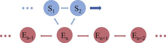
We consider a bipartite system S, consisting of a pair of two-level subsystems S₁ and S₂ with different frequencies ω₁ and ω₂, which are coupled to a common environment E, consisting of a sequence of identical ancillae (E₁, E₂, ..., E_n). We assume that there is no initial correlation between the two subsystems or the environment ancillae. Within the framework of collision model, we investigate the transient spontaneous synchronization between the two subsystems. The dynamic process is composed of a series repeated steps. In the nth step of the dynamics, S₁ and S₂ interact with the same environment ancilla E_n sequentially. Then after a free evolution of the whole system S, two adjacent environment ancillae E_n and E_n+1 interact with each other. And this process is repeated to the next environment ancilla E_n+1. In figure 1, the detail of the collision model and the interaction process is shown.

Figure 1.

New window|Download| PPT slide
Figure 1.Sketch of a bipartite system S made up of two subsystems S₁ and S₂ interacting with the environment ancillae sequentially. In the nth step of the dynamics, S₁ interacts with E_n; S₂ interacts with E_n; and followed by a free evolution of the system S; next, two adjacent environment ancillae E_n and E_n+1 interact with each other. Then S₁ and S₂ shift by one site, and this process is repeated to the (n + 1)th ancilla.


The free evolution of system S is characterized by the Hamiltonian(1)$\begin{eqnarray}{\hat{H}}_{{s}_{1}{s}_{2}}=\displaystyle \frac{\lambda }{2}({\hat{\sigma }}_{{s}_{1}}^{x}{\hat{\sigma }}_{{s}_{2}}^{x}+{\hat{\sigma }}_{{s}_{1}}^{y}{\hat{\sigma }}_{{s}_{2}}^{y})+\displaystyle \frac{{\omega }_{1}}{2}{\hat{\sigma }}_{{s}_{1}}^{z}+\displaystyle \frac{{\omega }_{2}}{2}{\hat{\sigma }}_{{s}_{2}}^{z},\end{eqnarray}$where ${\hat{\sigma }}^{x}$, ${\hat{\sigma }}^{y}$, ${\hat{\sigma }}^{z}$ are the Pauli operators, λ characterizes the coupling strength between S₁ and S₂. The corresponding unitary evolution operator is ${\hat{U}}_{{s}_{1}{s}_{2}}=\exp (-{\rm{i}}{\hat{H}}_{{s}_{1}{s}_{2}}\delta {t}_{{s}_{1}{s}_{2}})$ (setting ℏ = 1), and $\delta {t}_{{s}_{1}{s}_{2}}$ is the time interval of the free evolution of S₁ and S₂. The detune between the subsystems Δ = ω₂ − ω₁.

The interaction between S₁ and the nth environment ancilla E_n is described by the Hamiltonian(2)$\begin{eqnarray}{\hat{H}}_{{s}_{1}n}=\displaystyle \frac{J}{2}({\hat{\sigma }}_{{s}_{1}}^{x}{\hat{\sigma }}_{n}^{x}+{\hat{\sigma }}_{{s}_{1}}^{y}{\hat{\sigma }}_{n}^{y})+{\hat{H}}_{{s}_{1}{s}_{2}},\end{eqnarray}$where J characterizes the coupling strength between the subsystem and the environment ancilla E_n. The corresponding unitary evolution operator is written as ${\hat{U}}_{{s}_{1}n}=\exp (-{\rm{i}}{\hat{H}}_{{s}_{1}n}\delta {t}_{{s}_{1}n})$ with $\delta {t}_{{s}_{1}n}$ characterizing the time interval of the coupling between S₁ and the environment ancilla E_n. Similarly(3)$\begin{eqnarray}{\hat{H}}_{{s}_{2}n}=\displaystyle \frac{J}{2}({\hat{\sigma }}_{{s}_{2}}^{x}{\hat{\sigma }}_{n}^{x}+{\hat{\sigma }}_{{s}_{2}}^{y}{\hat{\sigma }}_{n}^{y})+{\hat{H}}_{{s}_{1}{s}_{2}},\end{eqnarray}$and the corresponding unitary evolution operator is ${\hat{U}}_{{s}_{2}n}\,=\exp (-{\rm{i}}{\hat{H}}_{{s}_{2}n}\delta {t}_{{s}_{2}n})$, with $\delta {t}_{{s}_{2}n}$ characterizing the time interval of the coupling between S₂ and the environment ancilla E_n. Then we obtain the total unitary evolution operator of the subsystems S₁, S₂ and the environment ancilla E_n, $\hat{U}={\hat{U}}_{{s}_{1}n}{\hat{U}}_{{s}_{2}n}{\hat{U}}_{{s}_{1}{s}_{2}}$, and the corresponding dynamic map of the interaction between the system S and the environment ancilla E_n can be written as(4)$\begin{eqnarray}{\varphi }_{s,n}(\rho )=\hat{U}\rho {\hat{U}}^{\dagger }.\end{eqnarray}$

Next, we introduce an interaction between two adjacent environment ancillae E_n and E_n+1, and assume that the corresponding unitary evolution operator is(5)$\begin{eqnarray}{\hat{U}}_{n,n+1}(\gamma )=\cos \gamma \hat{{\mathbb{I}}}+\mathrm{isin}\gamma {\hat{S}}_{n,n+1}.\end{eqnarray}$Here ${\hat{S}}_{n,n+1}$ is the SWAP gate, and in the ordered basis {∣0⟩, ∣1⟩} it reads(6)$\begin{eqnarray}{\hat{S}}_{n,n+1}=\left(\begin{array}{cccc}1 & 0 & 0 & 0\\ 0 & 0 & 1 & 0\\ 0 & 1 & 0 & 0\end{array}\right).\end{eqnarray}$Moreover, $\hat{{\mathbb{I}}}$ is the identity operator, and γ is a dimensionless interaction strength between the environment ancillae E_n and E_n+1. The corresponding dynamic map could be written as(7)$\begin{eqnarray}{\psi }_{n,n+1}(\rho )={\hat{U}}_{n,n+1}(\gamma )\rho {\hat{U}}_{n,n+1}^{\dagger }(\gamma ).\end{eqnarray}$When γ = 0, there is no information exchange between two adjacent environment ancillae, and the dynamic process is Markovian. When $\gamma =\tfrac{\pi }{2}$, there is a maximal information exchange between two adjacent environment ancillae, so the dynamic process becomes fully non-Markovian.

Furthermore, we retain the nth sub-environment freedom until the system interacts with the (n + 1)th sub-environment, i.e. the correlation established after S colliding with E_n+1 is erased only after E_n+1 has collided with E_n. The dynamic map resulting from this implementation thus gives rise to the reduced state of the system(8)$\begin{eqnarray}{\rho }_{s}={\mathrm{Tr}}_{n-1,n}({\psi }_{n-1,n}[{\varphi }_{s,n}[{\mathrm{Tr}}_{n-2}({\rho }_{n-1}^{{se}})\otimes {\rho }_{n}]]),\end{eqnarray}$where ${\mathrm{Tr}}_{n-2}[\cdot ]$ denotes the partial trace over the (n − 2)th environment ancilla prior to the interaction between S and E_n−1, and ${\rho }_{n-1}^{{se}}$ is the density matrix of system and the (n − 1)th environment ancilla. Then the initial state of next step of the dynamics can be written as ρ_s ⨂ ρ_n+1, where ρ_n+1 is the density matrix of a fresh environment unit.

3. Result

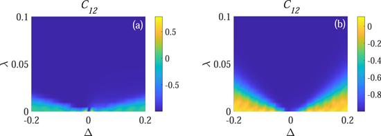
In this paper we use the Pearson coefficient [6] to characterize the degree of synchronization between the local observables of the subsystems. Given variables x and y, it can be expressed as(9)$\begin{eqnarray}{C}_{12}=\displaystyle \frac{{{\rm{\Sigma }}}_{i=1}^{n}({x}_{i}-\bar{x})({y}_{i}-\bar{y})}{\sqrt{{{\rm{\Sigma }}}_{i=1}^{n}{\left({x}_{i}-\bar{x}\right)}^{2}{{\rm{\Sigma }}}_{i=1}^{n}{\left({y}_{i}-\bar{y}\right)}^{2}}},\end{eqnarray}$where $\bar{x}$ and $\bar{y}$ are the mean values of x and y respectively, and n is the number of values the variables can take. C₁₂ = 0 indicates there is no synchronization between the subsystems; C₁₂ = 1 indicates synchronization; and C₁₂ = −1 indicates anti-synchronization. Without lose of generality, in this paper we choose $\langle {\sigma }^{x}\rangle =\mathrm{Tr}[{\rho }_{s}{\sigma }^{x}]$ as the local observable to witness the synchronization between S₁ and S₂. In numerical calculation we can not take the summations in equation (9) over the whole data set and generally take a part of it. To avoid sharp fluctuations of C₁₂, we take the average value of the nearest 140 data points as one value of the Pearson coefficient, and then calculate the next value of the nearest 140 data points with an interval of 15 data points from the first data point of the prior data set, to obtain another value of the Pearson coefficient. In this way, a smooth curve of C₁₂ can be obtained [62].

In the following, we investigate the synchronization between S₁ and S₂, and compare the behavior of synchronization in the Markovian regime and non-Markovian regime. We suppose that the initial state of the system is $\tfrac{1}{\sqrt{2}}(| 0\rangle +| 1\rangle )\otimes \tfrac{1}{\sqrt{2}}(| 0\rangle +| 1\rangle )$. Meanwhile, we assume that the environment ancillae are identical and in the same initial state ρ_e = ∣0⟩⟨0∣. From the numerical calculation, we find that the time for the subsystems to get anti-synchronized is different for different parameter region. In the parameter region of small λ and large Δ, even though the Pearson coefficient can eventually approaches −1 with a long enough evolution time, the expectation values of the local observables become extremely small. In other words, the system has reached its steady state before the transient synchronization appears. We argue that in this case even though the Pearson coefficient can arrive at −1 finally, there is no visibility for this anti-synchronization. So in this paper when the Pearson coefficient has not reached −1 before the expectation value of the local observable decays to 10⁻⁴ of the initial value, we say that the two qubits can not be synchronized. It is worth emphasizing that the magnitude of this value makes no qualitative difference to the following results in this paper. In figure 2(a) we display the behavior of Pearson coefficient between S₁ and S₂ in terms of detune Δ and coupling strength between two qubits λ in the Markovian regime (γ = 0). Without lose of generality, we suppose that the coupling strength between the subsystems and the environment ancilla J = 0.3ω, and ω₁ = ω. To avoid the situation of extremely small expectation values of local observables, the final collision times we choose N = 5000. As expected, we obtain a typical Arnold tongue which is shown in figure 2(a). It can be seen that the two subsystems tend to anti-synchronize in most area of parameter region except for very small values of λ and large values of Δ. Only when the coupling strength between S₁ and S₂ is strong enough to compensate the effect of detune, the anti-synchronization appears. When we increase N a little, the blue region in figure 2(a) would increase slightly. While as N increases further we find that although some region (especially the region with small λ and large Δ) turns into blue, i.e. C₁₂ ∼ − 1, the expectation value of the local observables would be extremely small before that. In this case there is no visibility of the synchronization, and according to our argument we say that it can not get anti-synchronized. From numerical calculation we find that by considering the visibility of synchronization when N > 5000, the result makes no qualitative difference from figure 2(a).

Figure 2.

New window|Download| PPT slide
Figure 2.The Pearson coefficient as a function of Δ and λ. For (a) γ = 0, and (b) $\gamma =\tfrac{\pi }{4}$. We set J = 0.3ω, ω₁ = ω, N = 5000, and $\omega \delta {t}_{{s}_{1}n}=\omega \delta {t}_{{s}_{2}n}=\omega \delta {t}_{{s}_{1}{s}_{2}}=0.2$.


Next, we turn our attention to studying the effect of non-Markovianity on the synchronization between S₁ and S₂ by considering a nonzero γ. In figure 2(b), we show the behavior of Pearson coefficient between S₁ and S₂ in terms of Δ and λ in the non-Markovian regime. Without lose of generality, we set $\gamma =\tfrac{\pi }{4}$, and the other parameters are the same as in figure 2(a). In the yellow region of figure 2(b), the two subsystems have not gotten anti-synchronized at N = 5000. Similar to figure 2(a) as we mentioned above, the blue region would be enlarged for a longer evolution time but by considering the visibility of synchronization the result remains qualitatively unchanged despite the quantitative differences to figure 2(b). Comparing figures 2(a) and (b), we can find that the region of emergence of anti-synchronization is decreased compared with that in the Markovian regime. It is easy to see that the non-Markovianity hinder the emergence of anti-synchronization between the two qubits.

From the above discussion, we argue that the Pearson coefficient can not fully characterize the synchronization between the subsystems. In the parameter region that C₁₂ ∼ −1, the amplitude of the expectation value of local observables can well reflect the visibility of synchronization phenomenon as an auxiliary. We define the visibility of synchronization ${ \mathcal V }$ as the average absolute value of the expectation value of the local observables(10)$\begin{eqnarray}{{ \mathcal V }}_{N}=\mathop{\max }\limits_{\{N\leqslant i\lt N+M\}}\{\displaystyle \frac{1}{2}(| \langle {\sigma }_{{s}_{1}}^{x}{\rangle }_{i}| +| \langle {\sigma }_{{s}_{2}}^{x}{\rangle }_{i}| )\}.\end{eqnarray}$To avoid sharp fluctuation of ${ \mathcal V }$, in the numerical calculation we divide the data points into a series of continuous subsets and each subset contain M data points, then we take the maximum value of each subset as one value of ${ \mathcal V }$. In this paper without lose of generality, we set M = 20. In the region that the Pearson coefficient approaches −1, a bigger value of ${ \mathcal V }$ characterizes a more apparent anti-synchronization phenomenon.

Next, we tend to investigate the relation among the visibility of synchronization, entanglement and quantum mutual information in both Markovian and non-Markovian regimes. In our analysis, we use concurrence [63] to measure the degree of entanglement, which is defined as(11)$\begin{eqnarray}E({\rho }_{s})=\max \{0,\sqrt{{\lambda }_{1}}-\sqrt{{\lambda }_{2}}-\sqrt{{\lambda }_{3}}-\sqrt{{\lambda }_{4}}\},\end{eqnarray}$where λ_i are the eigenvalue of ${\rho }_{s}\tilde{{\rho }_{s}}$ in the decreasing order. $\tilde{{\rho }_{s}}=({\sigma }^{y}\otimes {\sigma }^{y}){\rho }_{s}^{* }({\sigma }^{y}\otimes {\sigma }^{y})$ where ${\rho }_{s}^{* }$ is the complex conjugation of ρ_s. The quantum mutual information [64] is defined as(12)$\begin{eqnarray}I({\rho }_{s})=S({\rho }_{{s}_{1}})+S({\rho }_{{s}_{2}})-S({\rho }_{s}),\end{eqnarray}$where S(ρ_s) is the von Neumann entropy.

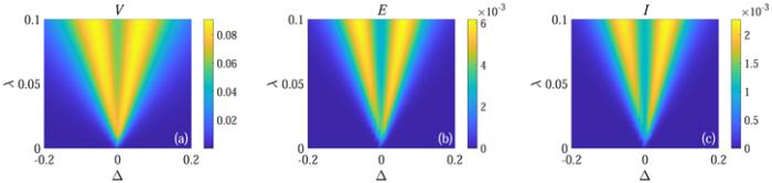
In figure 3, we plot ${ \mathcal V }$, entanglement and quantum mutual information as functions of Δ and λ in the Markovian regime (γ = 0). It can be seen from figure 3(a) that ${ \mathcal V }$ is small in the region of large Δ and small λ, which corresponds to the region that S₁ and S₂ can not get anti-synchronized. For weak coupling strength between S₁ and S₂, ${ \mathcal V }$ has a relative larger value when they are close to resonant. With the increase of λ, ${ \mathcal V }$ has a relative larger value when the subsystems are a little detuned. With further increase of λ, the value of Δ at which the maximum value of ${ \mathcal V }$ arrived at is increasing. Meanwhile, the behavior of entanglement and quantum mutual information are shown in figures 3(b) and (c), respectively. Obviously, there is an apparent link between the visibility of synchronization, entanglement and quantum mutual information, and the behavior of them are approximately the same. That means in this case entanglement and quantum mutual information can reflect the visibility of the synchronization. In the previous studies, the relation among the Pearson coefficient, entanglement and quantum mutual information has been investigated widely. However, comparing figures 2 with 3, we find that the connection among the Pearson coefficient, entanglement and quantum mutual information is not obvious.

Figure 3.

New window|Download| PPT slide
Figure 3.The diagram (a)–(c) display ${ \mathcal V }$, concurrence and quantum mutual information as functions of Δ and λ in the Markovian regime (γ = 0), respectively. We set J = 0.3ω, ω₁ = ω, N = 5000, and $\omega \delta {t}_{{s}_{1}n}=\omega \delta {t}_{{s}_{2}n}=\omega \delta {t}_{{s}_{1}{s}_{2}}=0.2$.


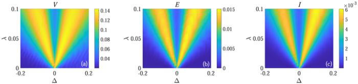
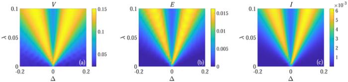
Next, we investigate the relation among ${ \mathcal V }$, entanglement and quantum mutual information in the non-Markovian regime. In figure 4, we plot ${ \mathcal V }$, entanglement and quantum mutual information with $\gamma =\tfrac{\pi }{4}$. The behavior of ${ \mathcal V }$ is consistent with entanglement and quantum mutual information once again. Comparing with figure 3, we find that the values of ${ \mathcal V }$, concurrence and quantum mutual information in the non-Markovian regime are apparently larger than their Markovian counterpart. From numerical calculation we find that S₁ and S₂ approximately arrive at anti-synchronization with the collision times N ∼ 5000 in the non-Markovian regime. As in the Markovian regime, when N ∼ 2000 the subsystems approximately arrive at anti-synchronization. We display the synchronization between S₁ and S₂ in the Markovian regime at N = 2000 in figure 5. Comparing figures 4 and 5, we can find that the behavior of ${ \mathcal V }$, concurrence and quantum mutual information in the non-Markovian regime are very similar to that in the Markovian regime including the magnitude of those values. As we know, ${ \mathcal V }$, concurrence and quantum mutual information will decay as time evolves, but due to the information backflow in the non-Markovian regime they will decay slower than that in the Markovian regime. Thus, it takes more time for ${ \mathcal V }$, concurrence and quantum mutual information in the non-Markovian regime to decay to the same level as those in the Markovian regime. That is the reason why the non-Markovianity delay the phenomenon of anti-synchronization between the subsystems.

Figure 4.

New window|Download| PPT slide
Figure 4.The diagram (a)–(c) display ${ \mathcal V }$, concurrence and quantum mutual information as functions of Δ and λ in the non-Markovian regime ($\gamma =\tfrac{\pi }{4}$), respectively. We set J = 0.3ω, ω₁ = ω, N = 5000, and $\omega \delta {t}_{{s}_{1}n}=\omega \delta {t}_{{s}_{2}n}=\omega \delta {t}_{{s}_{1}{s}_{2}}=0.2$.

Figure 5.

New window|Download| PPT slide
Figure 5.The diagram (a)–(c) display ${ \mathcal V }$, concurrence and quantum mutual information as functions of Δ and λ in the Markovian regime (γ = 0), respectively. We set J = 0.3ω, ω₁ = ω, N = 2000, and $\omega \delta {t}_{{s}_{1}n}=\omega \delta {t}_{{s}_{2}n}=\omega \delta {t}_{{s}_{1}{s}_{2}}=0.2$.


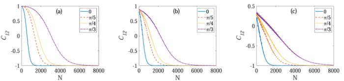
Next, we further investigate the effect of non-Markovianity on the synchronization when the subsystems are detuned. We show the time evolution of the Pearson coefficient for different Δ in figure 6. Different color characterize different inner-environment interaction strength γ: the blue solid line characterizes γ = 0, which means the environment is Markovian; the orange dashed lines, yellow dotted lines and purple dashed–dotted lines characterize $\gamma =\tfrac{\pi }{5},\tfrac{\pi }{4},\tfrac{\pi }{3}$ respectively, which indicate the non-Markovian environments. It can be seen from figure 6(a) that, in the case of resonance, the Pearson coefficient changes from 1 to −1 as time evolves, which indicates that S₁ and S₂ are synchronized at the beginning, and after a transient time, the two subsystems S₁ and S₂ lose their synchronization and gradually get anti-synchronized. In figures 6(b) and (c), we display C₁₂ for Δ = 0.05ω and Δ = 0.2ω, respectively. For a given Δ, from numerical calculation, we find that the non-Markovianity always delay the emergence of anti-synchronization, and it takes more time for S₁ and S₂ to get anti-synchronized with the increase of γ. On the other hand, for different Δ, two qubits S₁ and S₂ still arrive at anti-synchronization early in the Markovian regime compared with that in the non-Markovian regime. Compared with resonance, there is no obvious change in the time to get anti-synchronization for small Δ whether in the Markovian or non-Markovian regimes (see figure 6(b)), while it is slower to get anti-synchronized with large Δ for fixed γ (see figure 6(c)). Thus combine with figure 2, we can conclude that the detune between two qubits not only affects the degree of anti-synchronization, but also the time arriving at anti-synchronization.

Figure 6.

New window|Download| PPT slide
Figure 6.The Pearson coefficient as a function of the collision times N for different Δ. In (a) Δ = 0, (b) Δ = 0.05ω, and (c) Δ = 0.2ω. The blue solid lines, orange dashed lines, yellow dotted lines and purple dashed–dotted lines characterize γ = 0, $\gamma =\tfrac{\pi }{5}$, $\gamma =\tfrac{\pi }{4}$, $\gamma =\tfrac{\pi }{3}$ respectively. We set J = 0.3ω, λ = 0.1ω, ω₁ = ω, and $\omega \delta {t}_{{s}_{1}n}=\omega \delta $ ${t}_{{s}_{2}n}=\omega \delta {t}_{{s}_{1}{s}_{2}}=0.2$.


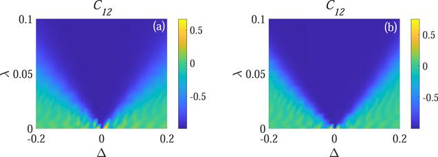
In the following, we investigate the effect of environment temperature on synchronization in the Markovian and non-Markovian regimes. We assume that the initial state of every identical environment ancilla is a thermal state ${\rho }_{e}=\tfrac{{{\rm{e}}}^{-\beta \omega {\sigma }^{z}}}{\mathrm{Tr}[{{\rm{e}}}^{-\beta \omega {\sigma }^{z}}]}$, where $\beta =\tfrac{1}{T}$ (we let k = 1). And ω is the frequency of the identical environment ancilla. Obviously, in the limit T → 0, the initial state of every identical environment ancilla reduces to ρ_e = ∣0⟩⟨0∣. From numerical calculation we find that the synchronization between S₁ and S₂ for low temperature is similar to that when every ancilla of the environment is in the vacuum state. With the increase of T, we find that the region of the emergence of anti-synchronization is decreased gradually. In figure 7, we show the Pearson coefficient as a function of Δ and λ for T = 5ω. Comparing figures 2 and 7, we can see that the region where C₁₂ ∼ −1 is decreased compared with that in vacuum environment whether in the Markovian regime or non-Markovian regime. Comparing figures 7(a) (γ = 0) and (b) ($\gamma =\tfrac{\pi }{4}$), we find that the behavior of Pearson coefficient in these two figures are similar for different Δ and λ. As expected, with the increase of T, the non-Markovianity becomes weak which leads to the behavior of synchronization in the non-Markovian regime approaches that in the Markovian regime. The increasing Δ always leads to the weakening of anti-synchronization between S₁ and S₂, and the magnitude of λ which can compensate the effect of detune strongly depends on the temperature, more specifically, the higher the temperature, the larger the λ for fixed Δ. Meanwhile, as we know that heat bath leads to the decoherence of system, and increasing the temperature of the bath will make the coherent oscillations of ⟨σ^x⟩ damping severely, thus the amplitude of ⟨σ^x⟩ decreases significantly with the increasing temperature. Accordingly, for a longer evolution time, although the region where C₁₂ ∼ −1 would be enlarged, the expectation value of the local observables would be extremely small before the Pearson coefficient approaches −1 in some region especially with large Δ and small λ.

Figure 7.

New window|Download| PPT slide
Figure 7.The Pearson coefficient as a function of Δ and λ with T = 5ω. In (a), γ = 0, and in (b), $\gamma =\tfrac{\pi }{4}$. We set J = 0.3ω, ω₁ = ω, N = 5000, and $\omega \delta {t}_{{s}_{1}n}=\omega \delta {t}_{{s}_{2}n}=\omega \delta {t}_{{s}_{1}{s}_{2}}=0.2$.


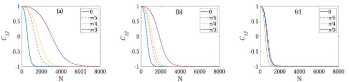
To further investigate the effect of temperature on synchronization in the Markovian and non-Markovian regimes, we show the time evolution of the Pearson coefficient for different T in figure 8. We can see from figure 8 that, with the increase of T, there is no obvious change for the time to get anti-synchronized in the Markovian regime (see the blue solid lines). But the two qubits arrive at anti-synchronization early in the non-Markovian regime for high temperature with the same γ, for example, the subsystems get anti-synchronized early with the increasing of T for $\gamma =\tfrac{\pi }{4}$ (see the yellow dotted lines). Thus the high temperature makes the synchronization in the non-Markovian regime with different γ close to that in the Markovian regime. Nevertheless, when the temperature is increased further, the magnitude of local observables would be extremely small before the Pearson coefficient approaches −1 in the most parameter region whether in the Markovian or non-Markovian regimes, and in this case the two qubits can not get anti-synchronized in the most region of the parameter space.

Figure 8.

New window|Download| PPT slide
Figure 8.The Pearson coefficient as a function of the collision times N for different T. In (a) T = 0.1ω, (b) T = ω, and (c) T = 5ω. The blue solid lines, orange dashed lines, yellow dotted lines and purple dashed–dotted lines characterize γ = 0, $\gamma =\tfrac{\pi }{5}$, $\gamma =\tfrac{\pi }{4}$, $\gamma =\tfrac{\pi }{3}$ respectively. We set J = 0.3ω, λ = 0.1ω, Δ = 0, and ωδ ${t}_{{s}_{1}n}=\omega \delta {t}_{{s}_{2}n}=\omega \delta {t}_{{s}_{1}{s}_{2}}=0.2$.


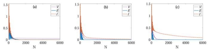
In figure 9 we plot ${ \mathcal V }$, entanglement and quantum mutual information as functions of N for different temperature. From numerical calculation, we find that with the increase of T, ${ \mathcal V }$ decreases as time evolves (see the purple dotted lines) because the incoherent pumping makes coherent oscillations of ⟨σ^x⟩ damping severely. When the amplitude of ⟨σ^x⟩ decays, the synchronization between the subsystems gradually loses their visibility. Besides, we can see from figure 9(a) that in the low temperature case, after a transient damped oscillations, the entanglement reduces to a small value. Comparing with figure 8, we find that the entanglement has not vanished before the Pearson coefficient reaches −1 (see the blue solid lines). When the temperature increases, it can be seen from figure 9(b) that the entanglement reduces to zero in a very short time, and has vanished before the emergence of anti-synchronization. With further increase of T, as shown in figure 9(c), the entanglement vanishes faster than that in figure 9(b). This is the well known phenomenon named entanglement sudden death (ESD) which has been investigated widely in the past few years [65]. For the model used in this paper, it is clear that the entanglement is not necessary for the anti-synchronization between the subsystems. Moreover, we can see from figure 9 that the quantum mutual information exhibit damped oscillations and then decrease rapidly for low temperature, but decays slowly with the increase of temperature (see the orange dashed–dotted lines). It is noted that for two qubits in the presence of of environment by using the Born–Markov master equation, a similar phenomenon that, the ESD emerges while the quantum mutual information still exists for high temperature of the environment has already been observed [66]. From above result it can be concluded that the increase of environment temperature breaks the correspondence among the visibility of synchronization, entanglement and quantum mutual information in our model.

Figure 9.

New window|Download| PPT slide
Figure 9.The diagram of ${ \mathcal V }$, entanglement and quantum mutual information as functions of the collision times N for different T. In (a) T = 0.1ω, (b) T = ω, and (c) T = 5ω. The purple dotted lines, blue solid lines and orange dashed–dotted lines characterize ${ \mathcal V }$, entanglement and quantum mutual information respectively. We set J = 0.3ω, λ = 0.1ω, Δ = 0, γ = 0 and $\omega \delta {t}_{{s}_{1}n}=\omega \delta $ ${t}_{{s}_{2}n}=\omega \delta {t}_{{s}_{1}{s}_{2}}=0.2$.

4. Conclusions

In this paper we have investigated the transient quantum spontaneous synchronization between two qubits interacting with a common non-Markovian environment based on a collision model. We have mainly explored the effect of non-Markovianity on the synchronization between two qubits. We have found that, in some situation, even though the Pearson coefficient approaches −1, there is no visibility of synchronization because the local observables are extremely small, and in this case we argue that the subsystems are not anti-synchronized. Thus, we defined ${ \mathcal V }$ to characterize the visibility of synchronization as an auxiliary after the Pearson coefficient C₁₂ ∼ −1. Particularly, we have found an obvious connection among ${ \mathcal V }$, entanglement and quantum mutual information when every environment ancilla is in the vacuum state whether in the Markovian or non-Markovian regimes. Comparing with the behavior of synchronization in the Markovian regime, we have found that the region of emergence of anti-synchronization is decreased in the non-Markovian regime. Meanwhile, it is always slower to get anti-synchronized in the non-Markovian regime compared with that in the Markovian regime, and with the increase of non-Markovianity, it takes more time for the subsystems to get anti-synchronized.

In addition, we have studied the effect of the environment temperature on the synchronization between the subsystems. With the increase of temperature, the behavior of synchronization in the non-Markovian regime gradually approaches that in the Markovian regime. Meanwhile, the high temperature decreases the parameter region of the emergence of anti-synchronization in both Markovian and non-Markovian regimes, and it also leads to the connection among ${ \mathcal V }$, entanglement and quantum mutual information broken.

Acknowledgments

This work is financially supported by the National Natural Science Foundation of China (Grant Nos. 11775019 and 11875086).

Reference View Option By original order
By published year
By cited within times
By Impact factor

[1]Pikovsky A Kurths J Rosenblum M 2002 Synchronization: a Universal Concept in Nonlinear Sciences vol 12 Cambridge Cambridge University Press
DOI:10.1119/1.1475332 [Cited within: 1]

[2]Huygens C 1665 letters no. 1333 of 24 February 1665, no. 1335 of 26 February 1665, and no. 1345 of 6 March 1665
Oeuvres Complites de Christiaan Huygens vol 8 Dordrecht Martinus Nijhoff
[Cited within: 1]

[3]Osipov G V Kurths J Zhou C 2007 Synchronization in Oscillatory Networks Berlin Springer
DOI:10.1007/978-3-540-71269-5 [Cited within: 1]

[4]Strogatz S H 2018 Nonlinear Dynamics and Chaos: with Applications to Physics, Biology, Chemistry, and Engineering Boulder, CO CRC Press
DOI:10.1201/9780429399640

[5]Arenas A Díaz-Guilera A Kurths J Moreno Y Zhou C 2008 Phys. Rep. 469 93
DOI:10.1016/j.physrep.2008.09.002 [Cited within: 1]

[6]Galve F Giorgi G L Zambrini R 2017 Quantum correlations and synchronization measures
Lectures on General Quantum Correlations and their Applications. Cham Springer 393 420
DOI:10.1007/978-3-319-53412-1_18 [Cited within: 2]

[7]Zhirov O V Shepelyansky D L 2008 Phys. Rev. Lett. 100 014101
DOI:10.1103/PhysRevLett.100.014101 [Cited within: 1]

[8]Zhirov O V Shepelyansky D L 2009 Phys. Rev. B 80 014519
DOI:10.1103/PhysRevB.80.014519

[9]Lee T E Sadeghpour H R 2013 Phys. Rev. Lett. 111 234101
DOI:10.1103/PhysRevLett.111.234101

[10]Walter S Nunnenkamp A Bruder C 2014 Phys. Rev. Lett. 112 094102
DOI:10.1103/PhysRevLett.112.094102

[11]Sonar S Hajdus̆ek M Mukherjee M Fazio R Vedral V Vinjanampathy S Kwek L 2018 Phys. Rev. Lett. 120 163601
DOI:10.1103/PhysRevLett.120.163601

[12]Goychuk I Casado-Pascual J Morillo M Lehmann J Hänggi P 2006 Phys. Rev. Lett. 97 210601
DOI:10.1103/PhysRevLett.97.210601

[13]Orth P P Roosen D Hofstetter W Hur K L 2010 Phys. Rev. B 82 144423
DOI:10.1103/PhysRevB.82.144423

[14]Bellomo B Giorgi G L Palma G M Zambrini R 2017 Phys. Rev. A 95 043807
DOI:10.1103/PhysRevA.95.043807

[15]Karpat G Yalçınkaya İ Cakmak B 2020 Phys. Rev. A 101 042121
DOI:10.1103/PhysRevA.101.042121 [Cited within: 1]

[16]Lee T E Chan C K Wang S 2014 Phys. Rev. E 89 022913
DOI:10.1103/PhysRevE.89.022913

[17]Es'haqi-Sani N Manzano G Zambrini R Fazio R 2020 Phys. Rev. Res. 2 023101
DOI:10.1103/PhysRevResearch.2.023101 [Cited within: 1]

[18]Xu M Tieri D A Fine E C Thompson J K Holland M J 2014 Phys. Rev. Lett. 113 154101
DOI:10.1103/PhysRevLett.113.154101

[19]Giorgi G L Galve F Manzano G Colet P Zambrini R 2012 Phys. Rev. A 85 052101
DOI:10.1103/PhysRevA.85.052101

[20]Manzano G Galve F Giorgi G L Hernández-García E Zambrini R 2013 Sci. Rep. 3 1439
DOI:10.1038/srep01439 [Cited within: 2]

[21]Roulet A Bruder C 2018 Phys. Rev. Lett. 121 063601
DOI:10.1103/PhysRevLett.121.063601

[22]Ludwig M Marquardt F 2013 Phys. Rev. Lett. 111 073603
DOI:10.1103/PhysRevLett.111.073603

[23]Hush M R Li W Genway S Lesanovsky I Armour A D 2015 Phys. Rev. A 91 061401(R)
DOI:10.1103/PhysRevA.91.061401

[24]Zhang J F Long G L Deng Z W Liu W Z Liu Z H 2004 Phys. Rev. A 70 062322
DOI:10.1103/PhysRevA.70.062322

[25]Kong X Y Xin T Wei S J Wang B X Wang Y Z Li K R Long G L 2018 Quantum Inf. Process. 17 297
DOI:10.1007/s11128-018-2057-9

[26]Liu X S Long G L Tong D M 2003 Simultaneous space and time synchronization using shared entangled qubits
Commun. Theor. Phys. 40 45 47
DOI:10.1088/0253-6102/40/1/45 [Cited within: 1]

[27]Qi Z T Li Y H Huang Y W Feng J Zheng Y L Chen X F 2021 arXiv:2106.13509v2
[Cited within: 1]

[28]Wang X F Sun X J Liu Y X Wang W Kan B X Dong P Zhao L L 2021 Transmission of photonic polarization states from geosynchronous Earth orbit satellite to the ground
Quantum Eng. 3 e73
DOI:10.1002/que2.73 [Cited within: 1]

[29]Laskar A W Adhikary P Mondal S Katiyar P Vinjanampathy S Ghosh S 2020 Phys. Rev. Lett. 125 013601
DOI:10.1103/PhysRevLett.125.013601 [Cited within: 1]

[30]Koppenhöfer M Bruder C Roulet A 2020 Phys. Rev. Res. 2 023026
DOI:10.1103/PhysRevResearch.2.023026 [Cited within: 2]

[31]Roulet A Bruder C 2018 Phys. Rev. Lett. 121 053601
DOI:10.1103/PhysRevLett.121.063601

[32]Jaseem N Hajdus̆ek M Vedral V Fazio R Kwek L C Vinjanampathy S 2020 Phys. Rev. E 101 020201(R)
DOI:10.1103/PhysRevE.101.020201 [Cited within: 1]

[33]Mari A Farace A Didier N Giovannetti V Fazio R 2013 Phys. Rev. Lett. 111 103605
DOI:10.1103/PhysRevLett.111.103605 [Cited within: 1]

[34]Giorgi G L Plastina F Francica G Zambrini R 2013 Phys. Rev. A 88 042115
DOI:10.1103/PhysRevA.88.042115 [Cited within: 1]

[35]Zhu B Schachenmayer J Xu M Herrera F Restrepo J G Holland M J Rey A M 2015 New J. Phys. 17 083063
DOI:10.1088/1367-2630/17/8/083063

[36]Ameri V Eghbali-Arani M Mari A Farace A Kheirandish F Giovannetti V Fazio R 2015 Phys. Rev. A 91 012301
DOI:10.1103/PhysRevA.91.012301 [Cited within: 1]

[37]Cabot A Galve F Zambrini R 2017 New J. Phys. 19 113007
DOI:10.1088/1367-2630/aa8b9c

[38]Cabot A Galve F Eguiluz V M Klemm K Maniscalco S Zambrini R 2018 Npj Quantum Inf. 4 57
DOI:10.1038/s41534-018-0108-9

[39]Siwiak-Jaszek S Olaya-Castro A 2019 Faraday Discuss. 216 38
DOI:10.1039/C9FD00006B

[40]Cabot A Giorgi G L Galve F Zambrini R 2019 Phys. Rev. Lett. 123 023604
DOI:10.1103/PhysRevLett.123.023604

[41]Eneriz H Rossatto D Z Cardenas-Lopez F A Solano E Sanz M 2019 Sci. Rep. 9 19933
DOI:10.1038/s41598-019-56468-x [Cited within: 1]

[42]Jaseem N Hajdus̆ek M Solanki P Kwek L C Fazio R Vinjanampathy S 2020 Phys. Rev. Res. 2 043287
DOI:10.1103/PhysRevResearch.2.043287 [Cited within: 1]

[43]Giorgi G L Cabot A Zambrini R 2019 Transient synchronization in open quantum systems
Advances in Open Systems and Fundamental Tests of Quantum Mechanics. Cham Springer 73 89
DOI:10.1007/978-3-030-31146-9_6 [Cited within: 1]

[44]Breuer H P Laine E M Piilo J Vacchini B 2016 Colloquium: non-Markovian dynamics in open quantum systems
Rev. Mod. Phys. 88 021002
DOI:10.1103/RevModPhys.88.021002 [Cited within: 1]

[45]de Vega I Alonso D 2017 Dynamics of non-Markovian open quantum systems
Rev. Mod. Phys. 89 015001
DOI:10.1103/RevModPhys.89.015001

[46]Li L Hall M J W Wiseman H M 2018 Phys. Rep. 759 1
DOI:10.1016/j.physrep.2018.07.001 [Cited within: 1]

[47]Karpat G Yalçınkaya İ Çakmak B Giorgi G L Zambrini R 2021 Synchronization and non-Markovianity in open quantum systems
Phys. Rev. A 103 062217 arxiv: 2008.03310v1
[Cited within: 2]

[48]Zhang S K Liu K Dong D Y Feng X X Pan F 2021 arxiv: 2101.00833v1
[Cited within: 1]

[49]Alicki R Lendi K 2007 Quantum Dynamical Semigroups and Applications, Lecture Notes in Physics vol 717 Berlin Springer
DOI:10.1007/3-540-70861-8_1 [Cited within: 1]

[50]Breuer H P Petruccione F 2002 Theory of Open Quantum Systems Oxford Oxford University Press
DOI:10.1093/acprof:oso/9780199213900.001.0001 [Cited within: 1]

[51]Ziman M Štelmachovič P Bužek V Hillery M Scarani V Gisin N 2002 Phys. Rev. A 65 042105
DOI:10.1103/PhysRevA.65.042105 [Cited within: 1]

[52]Scarani V Ziman M Štelmachovič P Gisin N Bužek V 2002 Phys. Rev. Lett. 88 097905
DOI:10.1103/PhysRevLett.88.097905

[53]Ziman M Štelmachovič P Bužek V 2003 J. Opt. B 5 S439
DOI:10.1088/1464-4266/5/3/383

[54]Ziman M Bužek V 2005 Phys. Rev. A 72 022110
DOI:10.1103/PhysRevA.72.022110

[55]Giovannetti V Palma G M 2012 Phys. Rev. Lett. 108 040401
DOI:10.1103/PhysRevLett.108.040401

[56]Giovannetti V Palma G M 2012 J. Phys. B 45 154003
DOI:10.1088/0953-4075/45/15/154003

[57]Ciccarello F Palma G M Giovannetti V 2013 Phys. Rev. A 87 040103(R)
DOI:10.1103/PhysRevA.87.040103

[58]Ciccarello F Giovannetti V 2013 Phys. Scr. 153 014010
DOI:10.1088/0031-8949/2013/T153/014010 [Cited within: 1]

[59]Lorenzo S Ciccarello F Palma G M 2016 Phys. Rev. A 93 052111
DOI:10.1103/PhysRevA.93.052111 [Cited within: 1]

[60]Rau J 1963 Phys. Rev. 129 1880
DOI:10.1103/PhysRev.129.1880 [Cited within: 1]

[61]McCloskey R Paternostro M 2014 Phys. Rev. A 89 052120
DOI:10.1103/PhysRevA.89.052120 [Cited within: 1]

[62]Karpat G Yalçınkaya İ Çakmak B 2019 Phys. Rev. A 100 012133
DOI:10.1103/PhysRevA.100.012133 [Cited within: 2]

[63]Wootters W K 1998 Phys. Rev. Lett. 80 2245
DOI:10.1103/PhysRevLett.80.2245 [Cited within: 1]

[64]Cerf N J Adami C 1998 Physica D 120 62
DOI:10.1016/S0167-2789(98)00045-1 [Cited within: 1]

[65]Yu T Eberly J H 2009 Science 323 5914
DOI:10.1126/science.1167343 [Cited within: 1]

[66]Chakrabarty I Banerjee S Siddharth N 2011 Quantum Inf. Comput. 11 541 562
[Cited within: 1]