Lei Sun, Wei Wang^,∗School of Science, Shenyang University of Technology, Shenyang 110870, China

First author contact: ^∗ Author to whom any correspondence should be addressed.
Received:2020-06-13Revised:2020-07-26Accepted:2020-08-11Online:2020-10-19


Abstract
Dynamic magnetic properties of the mixed-spin (3/2, 5/2) Ising graphene-like monolayer in an oscillating magnetic field are studied by means of Monte Carlo simulation. The effects of Hamiltonian parameters such as crystal field and time-dependent oscillating magnetic field on the dynamic order parameter, susceptibility and internal energy of the system are well presented and explained. Moreover, much attention has also been dedicated to the phase diagrams with different parameters in order to better comprehend the impacts of these parameters on the critical temperature. Our results reveal that the crystal fields of two sublattices have similar effects on the critical temperature, but the bias field and amplitude of oscillating field have opposite effects on it. We hope that our research can be of guiding significance to the theoretical and experimental studies of graphene-like monolayer.
Keywords： graphene-like monolayer;dynamic order parameter;susceptibility;phase diagram;Monte Carlo simulation


PDF (1006KB)MetadataMetricsRelated articlesExportEndNote|Ris|BibtexFavorite
Cite this article
Lei Sun, Wei Wang. Dynamic magnetic properties of Ising graphene-like monolayer. Communications in Theoretical Physics[J], 2020, 72(11): 115703- doi:10.1088/1572-9494/abb7d0

1. Introduction

Since Novoselov et al found monolayer graphene in 2004 with flying colors [1], graphene, as one of the most promising two-dimensional structures, has given rise to widespread concern. In view of its prominent physical and chemical characters [2 –4], graphene has potential applications on chemical engineering [5], sensors [6, 7], solar cells [8] and so on. In experiment, graphene has been prepared by applying various methods. Schniepp et al successfully manufactured functionalized graphene by stripping graphite oxide and finally found that it conducts electricity [9]. By employing chemical vapor deposition, planer nano-graphene from camphor was synthesized by Somani et al [10] In addition, Lotya et al prepared graphene as well through ultrasonic treatment of graphite in surfactant or water [11]. As is well-known, pure graphene cannot display magnetic properties spontaneously. However, Yazyev found that it can exhibit magnetic properties through reducing dimensions, disorder and other possible scenarios. Besides, he also elaborated on possible physical mechanisms of magnetic properties in some systems [12]. Through electrostatic stabilization, Li et al stressed that graphene sheets would become stable aqueous colloids [13]. These meaningful findings will effectively advance the study of graphene-related materials.

As a hot topic in the theoretical research of nanomaterials, mixed-spin systems have aroused wide concern and they have been used to study bimetallic molecular systems based magnetic materials. Recently, researchers have investigated the diverse mixed-spin Ising models, such as the mixed-spin (1/2, 1) nanowire [14], mixed-spin (2, 5/2) zigzag AFe_II Fe_III (C₂ O₄ )₃ nanoribbons [15], mixed-spin (5/2, 2) Kekulene structure [16], mixed-spin (1, 3/2) chain with inhomogeneous crystal-field anisotropy [17], mixed-spin (3/2, 2) Ising system with two alternative layers [18], mixed-spin (2, 5/2) Ising system on a graphene layer [19], mixed-spin (3, 7/2) bilayer decorated graphene structure [20] and so on. Specially, the mixed-spin (3/2, 5/2) Ising model has drawn great attention in recent years. Jiang et al used the effective-field theory (EFT) to probe the magnetic properties of mixed-spin (3/2, 5/2) nano-graphene bilayer and found that the blocking temperature increases with decreasing the transverse field whereas it is almost unchanged when the anisotropy is strong [21]. By applying mean field theory, Mohamad studied the magnetic properties of the mixed-spin (3/2, 5/2) system under the longitudinal field and illustrated the possibility of multiple compensation temperatures [22]. Recently, Monte Carlo (MC) simulation has been widely used in the research of mixed-spin nanomaterials. Masrour et al employed MC simulation to discuss magnetic properties of mixed-spin (3/2, 5/2) nano-graphene with defects. The rate defects dependence of magnetization was investigated in detail [23]. Similarly, they also researched the effect of physical parameters such as exchange couplings and crystal fields on total magnetization, critical temperature and magnetic hysteresis behaviors [24]. The magnetic behaviors of mixed-spin (3/2, 5/2) Ising system were studied by De La Espriella et al through MC simulation. The finite-temperature phase diagrams were given and the compensation temperatures were found and discussed [25]. Using the same method, Alzate-Cardona et al investigated the magnetic characteristics of a graphene layer with mixed-spin (3/2, 5/2) [26]. It was found that the critical and compensation temperatures dramatically altered with the variation of the exchange interaction.

Since the dynamical phase transition (DPT) was found by the method of EFT for the first time [27], the research on Ising model under oscillating magnetic field has attracted more and more attention. Ertas et al employed EFT to study the dynamic magnetic properties of the ferromagnetic triangular lattice under the oscillating external magnetic field and revealed the characteristics of dynamic phase diagrams and hysteresis behaviors of the system. Moreover, they also observed and discussed the tricritical point and reentrant behaviors [28]. In addition, the authors compared their results with those of in [29] in detail. They also investigated DPT as well as dynamic phase diagrams in the Blume–Capel model [30]. Their research revealed that the thermal behaviors rely on the interaction to a great extent. In addition, Ertas also explored the dynamical thermal characteristic in the square lattice [31]. Based on EFT, the dynamic magnetic behaviors of the site diluted ferromagnetic Ising model were investigated by AkIncI et al and they observed and discussed the reentrant phenomena [32]. Similarly using EFT, Benhouria et al also investigated dynamic magnetic properties of many low-dimensional nanomaterials such as multilayer nano-graphene [33], bilayer nano-graphene [34] and C₇₀ fullerene [35]. Additionally, Vatansever et al explored DPT in a quenched-bond diluted Ising ferromagnet and discussed dynamic properties of the different systems [36]. By means of MC simulation, Vatansever investigated DPT of the triangular lattice under an oscillating external magnetic field and found that the equilibrium system pertains to the same pervasiveness class [37]. Another interesting phenomenon that the increase of amplitude of the oscillating external magnetic field would break antiferromagnetism of the shell in nanoparticle was revealed as well, which resulted in the existence of a ground state with ferromagnetic property [38]. Moreover, Vatansever et al also stressed that the significance of the large amplitude of the oscillating external magnetic field on DPT in a spherical core–shell nanoparticle. There exist P-type, N-type and Q-type magnetic behaviors in the system under certain parametric conditions [39]. They also studied the dynamic magnetic properties of mixed-spin (1/2, 3/2) Ising ferrimagnetic system [40] and ferromagnetic thin film system [41] under an oscillating external magnetic field. Based on MC simulation, DPT in La_2/3 Ca_1/3 MnO₃ magnets was studied by Alzate-Cardona et al and typical conclusion was illustrated. It is found that the critical temperature increases with the decreasing of the amplitude of the external magnetic field and the strong time-dependent field causes disorder and so on [42].

In our previous studies, the magnetic behaviors of various nano-systems have been studied by means of MC simulation, such as the zigzag graphene nanoribbon (GRNs) [43], ferrimagnetic mixed-spin Ising nanoisland [44], nanowires [45], nanotubes [46], graphene-like nanoisland bilayer [47], nanoparticles [48] and so on. However, little attention has been applied to the dynamic magnetic properties of Ising graphene-like monolayer under external oscillating magnetic field. The kinetic Ising model can be used to analyze various biological, chemical and physical systems from theory [49]. In addition, it plays an important role in describing experimental observations as well. The investigations of DPT can bring forth new ideas in materials manufacturing, processing and nanotechnology, for instance the monomolecular organic films [50], pattern formation [51], cuprate superconductor [52].

As a result, the purpose of this paper is to reveal and explain the magnetization, magnetic susceptibility, internal energy and phase diagram of the mix-spin (3/2, 5/2) Ising graphene-like monolayer under different Hamiltonian parameters such as crystal field and external oscillating magnetic field through MC simulation. The paper is organized as follows: section 2 shows the model and MC simulation. In section 3, we exhibit and explain the typical results in detail. Finally, there is a brief conclusion in section 4 .

2. Model and MC simulation

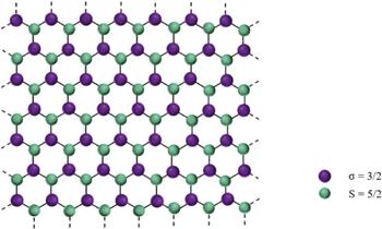
We considered a two-dimensional mixed-spin (3/2, 5/2) Ising model with graphene-like monolayer (see figure 1 ) under the time-dependent magnetic field h (t). It is composed of sublattice A (purple balls) with spin-3/2 and sublattice B (green balls) with spin-5/2. The lines connecting the sublattices represent the exchange couplings between the sublattices.

Figure 1.

New window|Download| PPT slide
Figure 1.Schematic of a ferrimagnetic mixed-spin (3/2, 5/2) Ising graphene monolayer.


The Hamiltonian of the considered system can be written as follows:(1)$ \begin{eqnarray}\begin{array}{rcl}H & = & -{J}_{{ab}}\displaystyle \sum _{\langle i,j\rangle }{\sigma }_{i}^{z}{S}_{j}^{z}-{D}_{a}\displaystyle \sum _{i}{\left({\sigma }_{i}^{z}\right)}^{2}\\ & & -{D}_{b}\displaystyle \sum _{j}{\left({S}_{j}^{z}\right)}^{2}-h(t)\left(\displaystyle \sum _{i}{\sigma }_{i}^{z}+\displaystyle \sum _{j}{S}_{j}^{z}\right),\end{array}\end{eqnarray}$ where $\langle ...\rangle $ is the sum of the spin.

${J}_{{ab}}$ : the exchange coupling between adjacent sublattices A and B.

D_a : the crystal field of the sublattice A.

D_b : the crystal field of the sublattice B.

The spin values of the sublattices A and B are ${\sigma }_{{ia}}^{z}=\pm 3/2,\pm 1/2$ and ${S}_{{jb}}^{z}=\pm 5/2,\pm 3/2,\pm 1/2$, respectively. h (t) is the external oscillating magnetic field and it can be represented as:(2)$ \begin{eqnarray}h(t)={h}_{b}+{h}_{0}\sin (\omega t).\end{eqnarray}$ Here, h_b denotes the bias field, h₀ represents oscillation amplitude and ω is the angular frequency of the oscillating magnetic field.

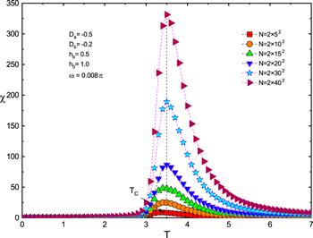
We performed MC simulation based on the Metropolis algorithm [53] to calculate the mixed-spin Ising model with high spin values. The periodic boundary conditions were employed on a 2N² honeycomb lattice. We carried out additional simulations to determine the system size. Figure 2 shows the temperature dependence of the susceptibility χ of the system for various system size 2N² with fixed D_a =−0.5, D_b =−0.2, h_b =0.5, h₀ =1.0 and ω =0.008π, respectively. It is found that there exists a peak in each χ curve no matter which system size. It is worth noting that the peak corresponds to the critical temperature T_C [35, 42, 54]. One can notice that the value of T_C increases with the increase of 2N² when 2N² <2×20², which suggests that the obvious finite size effect for small size. But no significant difference was found in the peak of the χ curve when the system size 2N² changes from 2×20² to 2×40² . Therefore, we selected the system size 2×20² in the following simulations for the sake of saving computing time because it is enough for reflecting the intrinsic properties of studied Hamiltonian. In one Monte Carlo step (MCS), each spin is swept independently and randomly. In order to get equilibrium of the system, we applied 5×10⁵ MCS to calculate the average value of thermodynamic quantity after eliminating first 2×10⁵ MCS at each temperature. The error bars are obtained by averaging 10 independent sample based on the Jackknife method [55, 56].

Figure 2.

New window|Download| PPT slide
Figure 2.The temperature dependence of χ for different system size 2N² with D_a =−0.5, D_b =−0.2, h_b =0.5, h₀ =1.0, ω =0.008π .


The interested quantities are calculated as follows:

The instantaneous internal energy of the system per spin can be expressed by:(3)$ \begin{eqnarray}E(t)=\displaystyle \frac{1}{2{N}^{2}}\langle H\rangle ,\end{eqnarray}$ where $\langle ...\rangle $ is the average value of the thermodynamic quantities.

The dynamical internal energy of the system per spin can be calculated as:(4)$ \begin{eqnarray}U=\displaystyle \frac{\omega }{2\pi }\oint E(t){\rm{d}}t.\end{eqnarray}$

The instantaneous magnetizations of the sublattice are given as:(5)$ \begin{eqnarray}{M}_{a}(t)=\displaystyle \frac{1}{{N}^{2}}\displaystyle \sum _{i}{\sigma }_{i}^{z},\end{eqnarray}$(6)$ \begin{eqnarray}{M}_{b}(t)=\displaystyle \frac{1}{{N}^{2}}\displaystyle \sum _{j}{S}_{j}^{z}.\end{eqnarray}$

The dynamic order parameters of the sublattices can be computed as follows:(7)$ \begin{eqnarray}{Q}_{a}=\displaystyle \frac{\omega }{2\pi }\oint {M}_{a}(t){\rm{d}}t,\end{eqnarray}$(8)$ \begin{eqnarray}{Q}_{b}=\displaystyle \frac{\omega }{2\pi }\oint {M}_{b}(t){\rm{d}}t.\end{eqnarray}$

In above equations, except the study of the effect of ω on the dynamical magnetic properties, the angular frequency of the oscillating magnetic field is taken $\omega =2\pi /\tau =2\pi /250=0.008\pi $ . Here, τ represents the period of the oscillating magnetic field and one complete oscillation would require 250 MCS. At first, we eliminated date for 800 such cycles. Then we used the rest 1200 cycles to calculate the dynamic order parameter Q_a of the sublattice A. Simulations show that the 1200 cycles are enough to get equilibrium of the system. Based on the same way, we can calculate the dynamic order parameter Q_b for the other sublattice B.

Therefore, the average dynamic order parameter of the system per spin is:(9)$ \begin{eqnarray}{Q}_{t}=\displaystyle \frac{{N}^{2}\times {Q}_{a}+{N}^{2}\times {Q}_{b}}{2{N}^{2}}.\end{eqnarray}$

The susceptibility of the system is defined as:(10)$ \begin{eqnarray}\chi =2\beta {N}^{2}\left(\langle {Q}_{t}^{2}\rangle -\langle {Q}_{t}{\rangle }^{2}\right),\end{eqnarray}$ where β denotes $\beta =\tfrac{1}{{k}_{{\rm{B}}}T}$, and the T is the absolute temperature. In addition, k_B represents Boltzmann constant. In order to facilitate the calculations, here we set up k_B =1.

3. Result and discussion

3.1. Dynamic order parameter, susceptibility and internal energy

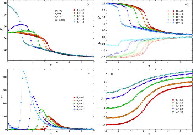
Figure 3 exhibits temperature dependence of the dynamic order parameter of the system ${Q}_{t}$, the dynamic order parameters of the sublattices Q_a, Q_b, susceptibility χ, and internal energy U for different values of D_a with D_b =−0.2, h_b =0.5, h₀ =1.0, ω =0.008π . In figure 3 (a), one can observe two saturation values (Q_t =0.5, 1.0) at zero temperature corresponding to two configurations of sublattice spin states (−3/2, 5/2) and (−1/2, 5/2) at the ground state, which can be calculated as: ${Q}_{t}=\tfrac{{20}^{2}\times (-1.5)+{20}^{2}\times 2.5}{2\,\times \,{20}^{2}}=0.5$ and ${Q}_{t}=\tfrac{{20}^{2}\times (-0.5)+{20}^{2}\times 2.5}{2\,\times \,{20}^{2}}=1.0$, respectively. Q_t curves with different values of D_a can display abundant changing profiles. It is clearly seen that the curves labeled D_a =−0.3, −1.0, −4.0 keep a downward trend all through as T increases until they are almost constant at high temperature region. However, a bulge which rises a little and then falls can be observed in the curves labeled D_a =−2.0, −3.0, which can be explained that frustrated spin states created by thermal agitation are released and different coexisting spin states are produced. As T increases, all of the Q_t curves change from their saturation values and finally converge to a non-zero constant value at high temperature region.This non-zero constant value results from the existence of h_b . In addition, when T >3.5, Q_t is the same at the same T no matter how large D_a is. This is because higher T can promote the spin value to zero and thus reduce Q_t . In the high temperature region, the influence of temperature rather than D_a on Q_t is dominant. Similar behaviors also have been found in the mixed-spin (1/2, 3/2) Ising ferrimagnetic system [40]. One can notice from figure 3 (b) that there exist two saturation values ${Q}_{a}=-0.5\left({D}_{a}=-4.0\right)$ and ${Q}_{a}=-1.5\left({D}_{a}=-0.3,-1.0,-2.0,-3.0\right)$ in Q_a curves and only one saturation value Q_b =2.5 in Q_b curves, which should be responsible for the formation of saturation values in figure 3 (a). It follows that strong crystal field (D_a =−4.0) forces the sublattice. A from high-spin state to low-spin state and then leads to the presence of various saturation values of Q_a . Figure 3 (c) shows the temperature dependence of χ curves for certain parameters. One can notice that there exist one or two peaks in each χ curve, it is worth noting that the peak at higher temperature corresponds to the critical temperature T_C . Obviously, T_C decreases monotonously with the increase of $\left|{D}_{a}\right|$ . Similar behavior has been observed in other theoretical studies of nano-structures [57 –60]. It is interesting that the peaks of the double-peak susceptibility curves at lower temperatures correspond to dramatic changes in the magnetization curve. It is remarkably that this double-peak phenomenon of susceptibility curves has been found by both MC simulation [61 –64] and EFT [18, 65]. It can be observed from figure 3 (d) that U increases with the increase of T . In addition, it also increases as $\left|{D}_{a}\right|$ increases, in other words, the strong crystal field makes the system unstable. Moreover, a flection point can be found in each U curve at T_C, which reflects that the process of phase transition is accompanied by the fluctuation of system energy.

Figure 3.

New window|Download| PPT slide
Figure 3.The temperature dependence of Q_t, Q_a, Q_b, χ and U for different values of D_a with D_b =−0.2, h_b =0.5, h₀ =1.0, ω =0.008π .


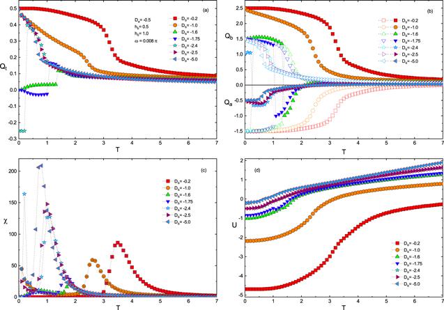
Figure 4 shows the temperature dependence of the Q_t, Q_a, Q_b, χ and U for diverse values of D_b with D_a =−0.5, h_b =0.5, h₀ =1.0, ω =0.008π . There are three saturation values(Q_t =0.5, 0, −0.25) in figure 4 (a), which can be calculated as: ${Q}_{t}=\tfrac{{20}^{2}\times (-1.5)+{20}^{2}\times 2.5}{2\,\times \,{20}^{2}}=0.5$ for D_b =−0.2, −1.0, ${Q}_{t}=\tfrac{{20}^{2}\times (-1.5)+{20}^{2}\times 1.5}{2\,\times \,{20}^{2}}=0$ for D_b =−1.6, −1.75, ${Q}_{t}=\tfrac{{20}^{2}\times (-1.5)+{20}^{2}\times 1.0}{2\,\times \,{20}^{2}}=-0.25$ for D_b =−2.4 and ${Q}_{t}=\tfrac{{20}^{2}\times (-0.5)+{20}^{2}\times 1.5}{2\,\times \,{20}^{2}}=0.5$ for D_b =−2.5, −5.0, respectively. It is worth mentioning that Q_t decreases with the increase of T as well as the decrease of $\left|{D}_{b}\right|$ for the curves Q_t labeled D_b =−0.2, −1.0, −2.5, −5.0. Obviously, an interesting turnover phenomenon will occur in Q_t curves for the values of D_b =−1.6, −1.75, −2.4. To be specific, for D_b =−1.6, the Q_t curve increases from its saturation value (Q_t =0) to a maximum and then drops and gets closer and closer to a certain value. The curve labeled D_b =−1.75 first decreases from Q_t =0 to a minimum value, then increases to a maximum and finally decreases and maintains a constant. Besides, for D_b =−2.4, Q_t increases from its saturation value (Q_t =−0.25) to its maximum, then gradually falls and finally keeps a constant. The effect of D_b on Q_a, Q_b presented in figure 4 (b) would take charge of variation of Q_t in figure 4 (a). In figure 4 (b), it is clearly observed that both Q_a and Q_b flip to the opposite direction at lower temperature when D_b =−1.6, −1.75, −2.4. The reasons of this phenomenon can be interpreted as: on the one hand, the larger value of $\left|{D}_{b}\right|$ will make the spin states of sublattice B from high to low as mentioned before. On the other hand, the reversal of Q_a, Q_b at low temperature can satisfy the lowest energy principle. Similar to figure 3 (c), the double-peak phenomenon of the χ curves also occurs in figure 4 (c). In addition, it can be found that the T_C decreases with the increase of $\left|{D}_{b}\right|$, which reflects that the strong crystal field can promote the occurrence of phase transition. Figure 4 (d) indicates that we can reduce the internal energy and promote the stability of the system through lowering the temperature or decreasing the crystal field.

Figure 4.

New window|Download| PPT slide
Figure 4.The temperature dependence of Q_t, Q_a, Q_b, χ and U for different values of D_b with D_a =−0.5, h_b =0.5, h₀ =1.0, ω =0.008π .


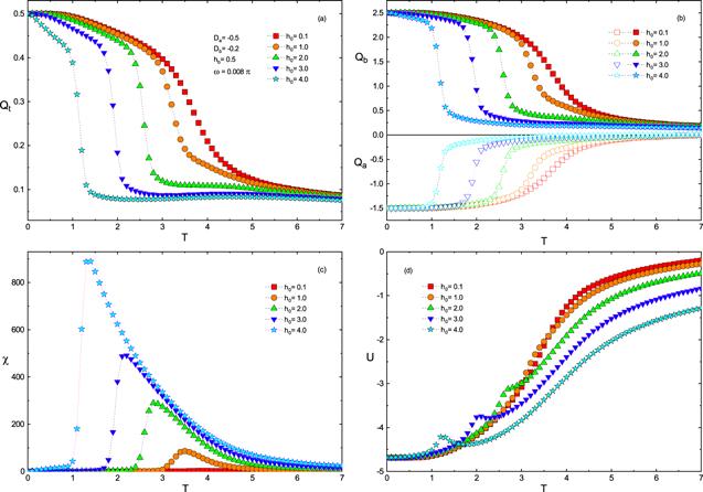
Figure 5 presents the impact of h_b on the Q_t, Q_a, Q_b, χ and U in the case of D_a =−0.5, D_b =−0.2, h₀ =1.0, ω =0.008π . Compared with figures 3 (a) and 4 (a), there is only one saturation value for all Q_t curves in figure 5 (a). When h_b is small (h_b =1.0, 1.5), Q_t decreases monotonically with the increase of T, while Q_t first rises and then falls with the increase of T for large h_b (h_b =2.0, 2.5, 3.0). Moreover, it is worth noting that the Q_t curves corresponding to different h_b are quite different at high temperature, which indicates that the bias field can affect the dynamic ordered parameters at high temperature significantly. In figure 5 (b), the saturation values of Q_a, Q_b (Q_a =−1.5 and Q_b =2.5) can take charge of the saturation value of Q_t, namely, ${Q}_{t}=\tfrac{{20}^{2}\times (-1.5)+{20}^{2}\times 2.5}{2\,\times \,{20}^{2}}=0.5$ by equation (9 ). Q_a and Q_b are not sensitive to the value of h_b in the low temperature zone (T <3.0), while both Q_a and Q_b decrease significantly with the increase of h_b for T >3.0. According to figure 5 (c), one can find that with the increase of h_b, χ decreases monotonically and the maximum of the χ curves moves towards right which suggests that T_C increases. The physical explanation is as follows: the strong bias field h_b can promote the direction of the spin to be uniform, thus a higher temperature is necessary for the system to undergo a phase transition. In figure 5 (d), one can intuitively observe that the U increases with the increase of T as well as the decrease of h_b .

Figure 5.

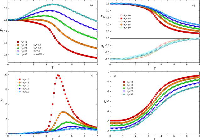New window|Download| PPT slide
Figure 5.The temperature dependence of Q_t, Q_a, Q_b, χ and U for different values of h_b with D_a =−0.5, D_b =−0.2, h₀ =1.0, ω =0.008π .


Figure 6 exhibits the Q_t, Q_a, Q_b, χ and U as the function of T for different h₀ with fixed values of D_a =−0.5, D_b =−0.2, h_b =0.5, ω =0.008π . It is clearly seen from figure 6 (a) that there is a common saturation value (Q_t =0.5) in the Q_t curves. Q_t decreases monotonically with the increase of T . Specifically, for example, for h₀ =2.0, Q_t decreases slowly with the increase of T when T <2.2, while it drops sharply at 2.2<T <3.0. When T >3.0, Q_t is no longer sensitive to the change of T . This indicates that Q_t can be mostly affected by T during middle temperature segment. Q_t decreases monotonically with increasing h₀ at a given temperature, which is contrary to the effect of h_b . Comparable results were also found in La_2/3 Ca_1/3 MnO₃ manganites [42]. One can deduce from figure 6 (b) that the influence of h₀ on Q_a and Q_b is more obvious compared with that of h_b, namely, with the increase of h₀, Q_a and Q_b gradually move to the left. It is discovered from figure 6 (c) that T_C decreases with the increase of h₀, which is also contrary to the effect of h_b . This finding is in accordance with the expectations. It is because of the fact that the magnetic energy originating from the external field dominants against the energy provided by exchange couplings with increasing h₀ . On account of this mechanism, the Ising graphene-like monolayer can relax within the oscillation period of the applied field so that the value of T_C decreases [66]. It is noteworthy from figure 6 (d) that there occur the fluctuations in the U curves in the low temperature region, because h₀ dominates U at low temperature rather than T . When h₀ is large (h₀ ≥2.0), the external magnetic field oscillates violently and it is easy to cause the energy fluctuations of the system in the low temperature region (T <3.0). When T is higher, T has a dominant effect on the energy of the system and the fluctuations disappear. The results are in great agreement with some previous studies [33, 34, 38, 40, 42].

Figure 6.

New window|Download| PPT slide
Figure 6.The temperature dependence of Q_t, Q_a, Q_b, χ and U for different values of h₀ with D_a =−0.5, D_b =−0.2, h_b =0.5, ω =0.008π .


Finally, figure 7 is depicted to show the effect of ω on the temperature dependence of Q_t, Q_a, Q_b, χ and U with fixed values of D_a =−0.5, D_b =−0.2, h_b =0.5, h₀ =1.0. In figure 7 (a), it is obvious that Q_t is insensitive to the changes of ω when T ≤2.7 or T ≥4.5, while it increases dramatically with the increase of ω when 2.7<T <4.5. This can be explained as follows: when ω is small, the external magnetic field oscillates slowly and the direction of the sublattice spin can follow the time-dependent magnetic field, causing the system in an ordered state with small Q_t . When ω is large, the direction of sublattice spin cannot keep up with the change of the external field, which leads to raise Q_t and undergo phase transition more difficultly. It is obvious in figure 7 (b) that both Q_a and Q_b decrease with the decrease of ω and the increase of T . In figure 7 (c), T_C increases with the increase of ω although that is not very obvious. In figure 7 (d), it is obvious that U is insensitive to changes of ω . However, from local enlargement one can clearly observe that the larger ω is, the larger U is in the higher temperature region.

Figure 7.

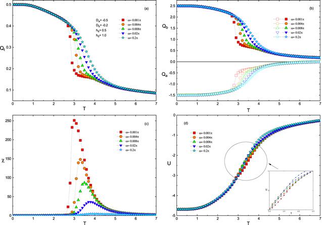New window|Download| PPT slide
Figure 7.The temperature dependence of Q_t, Q_a, Q_b, χ and U for different values of ω with D_a =−0.5, D_b =−0.2, h_b =0.5, h₀ =1.0.

3.2. Phase diagram

So as to better elucidate the effects of the various Hamiltonian parameters such as D_a, D_b, h_b, h₀ and ω on the T_C, the phase diagrams are given in figure 8 . Figures 8 (a) and (b) show the variation of T_C as the function of sublattice crystal fields D_a and D_b . It is obvious that T_C decreases monotonically with the increase of $\left|{D}_{a}\right|$ or $\left|{D}_{b}\right|$ . In addition, T_C is no longer sensitive to changes of $\left|{D}_{b}\right|$ when $\left|{D}_{b}\right|$ is large $(\left|{D}_{b}\right|\gt 2.7)$ . The influence of external magnetic field on T_C is shown in figures 8 (c) and (d). It should been mentioned that h_b and h₀ have opposite effects on T_C, which is because of their different roles as the parameters of the external magnetic field. As the bias field, h_b can tend to promote the spins of the sublattices to be unified along its direction and prevent the system from undergoing phase transition into a disorder. On the contrary, larger h₀ can break the order of the system easily so as to reduce T_C . We can remark that oscillating field causes disorder while bias field causes order for the system. Remarkably, it is necessary to underline that the function relation between T_C and h₀ is approximately linear, which is because the magnetic energy derived from Zeeman energy governs the energy produced by the spin interaction with the increase of h₀ . Similar results have been found in previous studies [38, 41, 42]. In figure 8 (e), T_C increases with the increase of ω, while it is no longer sensitive to the change of ω when ω >0.02π . The physical mechanism of this phenomenon can be described as: the large value of ω would lead to the short change period of the oscillating magnetic filed. Hence, the system magnetization cannot change immediately with the rapidly changing oscillating magnetic field, which results in that the external magnetic field has a slight influence on the T_C although h₀ is large. Similar results have been observed in [36, 67].

Figure 8.

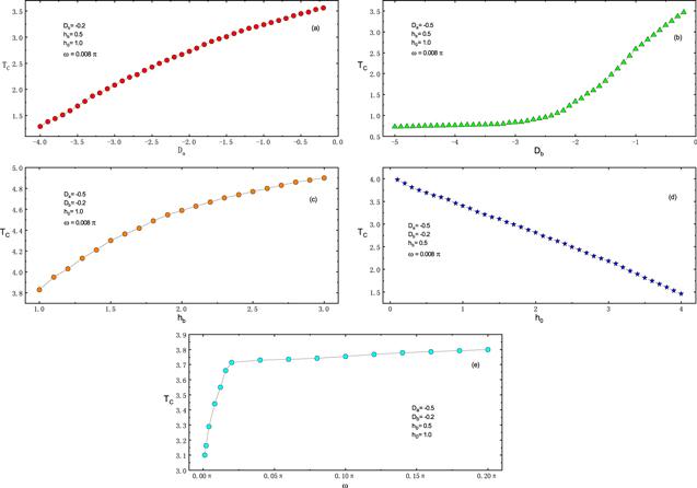New window|Download| PPT slide
Figure 8.The temperature dependence of D_a, D_b, h_b, h₀ and ω on the critical temperature T_C for (a) D_b =−0.2, h_b =0.5, h₀ =1.0, ω =0.008π ; (b) D_a =−0.5, h_b =0.5, h₀ =1.0, ω =0.008π ; (c) D_a =−0.5, D_b =−0.2, h₀ =1.0, ω =0.008π ; (d) D_a =−0.5, D_b =−0.2, h_b =0.5, ω =0.008π ; (e) D_a =−0.5, D_b =−0.2, h_b =0.5, h₀ =1.0.

4. Conclusion

In this investigation, the dynamic magnetic behaviors of the mixed-spin (3/2, 5/2) Ising graphene-like monolayer have been studied by employing the MC simulation. The temperature dependence of Q_t, Q_a, Q_b, χ and U for different values of Hamiltonian parameters such as D_a, D_b, h₀, h₀ and ω has been exhibited and elucidated in detail. Moreover, particular effort has also been dedicated to the phase diagrams with different planes of parameters so as to further explain the phase transition of the system. We found that D_a and D_b have similar effects on T_C, but h₀ and h_b have opposite effects on T_C . In addition, T_C is sensitive to the change of ω only when ω is rather small. We hope that our investigation will contribute to the further study of graphene-like monolayer.

Reference View Option By original order
By published year
By cited within times
By Impact factor

[1]Novoselov K S Geim A K Morozov S V Jiang D Zhang Y Dubonos S V Grigorieva I V Firsov A A 2004 Science 306 666
DOI:10.1126/science.1102896 [Cited within: 1]

[2]Masrour R Jabar A 2016 Super Micro 98 78
DOI:10.1016/j.spmi.2016.08.005 [Cited within: 1]

[3]Feraoun A Kerouad M 2018 Phys. Lett. A 382 116
DOI:10.1016/j.physleta.2017.10.040

[4]Masrour R Jabar A 2017 J. Comput. Electron. 16 576
DOI:10.1007/s10825-017-0990-y [Cited within: 1]

[5]Xu L J Chu W Gan L 2015 Chem. Eng. J. 263 435
DOI:10.1016/j.cej.2014.11.065 [Cited within: 1]

[6]Karpiak B Dankert A E Dash S P 2017 J. Appl. Phys. 122 054506
DOI:10.1063/1.4997463 [Cited within: 1]

[7]Koczorowski W et al. 2017 Mater. Sci. Semicond. Proc. 67 92
DOI:10.1016/j.mssp.2017.05.021 [Cited within: 1]

[8]Song Y Li X M Mackin C Zhang X Fang W J Palacios T Zhu H W Kong J 2015 Nano Lett. 15 2104
DOI:10.1021/nl505011f [Cited within: 1]

[9]Schniepp H C Li J L McAllister M J Sai H Alonso M H Adamson D H Prud’homme R K Car R Saville D A Aksay I A 2006 J. Phys. Chem. 110 8535
DOI:10.1021/jp060936f [Cited within: 1]

[10]Somani P R Somani S P Umeno M 2006 Chem. Phys. Lett. 430 56
DOI:10.1016/j.cplett.2006.06.081 [Cited within: 1]

[11]Lotya M Hernandez Y Coleman J 2009 J. Am. Chem. Soc. 131 3611
DOI:10.1021/ja807449u [Cited within: 1]

[12]Yazyev O V 2010 Rep. Prog. Phys. 73 056501
DOI:10.1088/0034-4885/73/5/056501 [Cited within: 1]

[13]Li D Mueller M B Gilje S 2008 Nat. Nanotechnol. 2 101
DOI:10.1038/nnano.2007.451 [Cited within: 1]

[14]Kantar E Kocakaplan Y 2015 J. Magn. Magn. Mater. 393 574
DOI:10.1016/j.jmmm.2015.06.009 [Cited within: 1]

[15]Drissi L B Zriouel S Nit Ben Ahmed H 2018 J. Magn. Magn. Mater. 449 328
DOI:10.1016/j.jmmm.2017.10.045 [Cited within: 1]

[16]Jabar A Masrour R 2019 Physica A 514 974
DOI:10.1016/j.physa.2018.09.125 [Cited within: 1]

[17]Solano-Carrillo E Franco R Silva-Valencia J 2010 J. Magn. Magn. Mater. 322 1917
DOI:10.1016/j.jmmm.2010.01.007 [Cited within: 1]

[18]Deviren B Polat Y Keskin M 2011 Chin. Phys. B 20 060507
DOI:10.1088/1674-1056/20/6/060507 [Cited within: 2]

[19]Feraoun A Amraoui S Kerouad M 2019 Chin. J. Phys. 58 98
DOI:10.1016/j.cjph.2018.12.024 [Cited within: 1]

[20]Tahiri N Jabar A Bahmad L 2017 Phys. Lett. 381 189
DOI:10.1016/j.physleta.2016.11.011 [Cited within: 1]

[21]Jiang W Yang Y Y Guo A B 2015 Carbon 95 190
DOI:10.1016/j.carbon.2015.07.097 [Cited within: 1]

[22]Mohamad H K 2011 J. Magn. Magn. Mater. 323 61
DOI:10.1016/j.jmmm.2010.08.030 [Cited within: 1]

[23]Masrour R Bahmad L Benyoussef A Hamedoun M Hlil E K 2013 J. Supercond. Nov. Magn. 26 679
DOI:10.1007/s10948-012-1785-9 [Cited within: 1]

[24]Jabar A Masrour R 2016 J. Supercond. Nov. Magn. 29 1363
DOI:10.1007/s10948-016-3417-2 [Cited within: 1]

[25]De La Espriella N Buendia G M 2011 J. Phys.: Condens. Matter 23 176003
DOI:10.1088/0953-8984/23/17/176003 [Cited within: 1]

[26]Alzate-Cardona J D Sabogal-Suarez D Restrepo-Parra E 2017 J. Magn. Magn. Mater. 429 34
DOI:10.1016/j.jmmm.2017.01.004 [Cited within: 1]

[27]Tome T de Oliveira M J 1990 Phys. Rev. A 41 4251
DOI:10.1103/PhysRevA.41.4251 [Cited within: 1]

[28]Ertas M Kantar E Kocakaplan Y Keskin M 2016 Physica A 444 732
DOI:10.1016/j.physa.2015.10.069 [Cited within: 1]

[29]Korniss G Rikvold P A Novotny M A 2002 Phys. Rev. E 66 056127
DOI:10.1103/PhysRevE.66.056127 [Cited within: 1]

[30]Ertas M Keskin M Deviren B 2012 J. Magn. Magn. Mater. 324 1503
DOI:10.1016/j.jmmm.2011.11.043 [Cited within: 1]

[31]Ertas M 2018 Physica B 550 154
DOI:10.1016/j.physb.2018.08.053 [Cited within: 1]

[32]AkIncI U Yvksel Y Vatansever E Polat H 2012 Physica A 391 5810
DOI:10.1016/j.physa.2012.06.060 [Cited within: 1]

[33]Benhouria Y Khossossi N Houmad M Essaoudi I Ainane A Ahuja R 2019 Physica E 105 139
DOI:10.1016/j.physe.2018.09.008 [Cited within: 2]

[34]Benhouria Y Bouziani I Essaoudi I Ainane A Ahuja R 2018 J. Magn. Magn. Mater. 460 223
DOI:10.1016/j.jmmm.2018.04.007 [Cited within: 2]

[35]Benhouria Y Essaoudi I Ainane A Ahuja R 2019 Physica E 108 191
DOI:10.1016/j.physe.2018.11.043 [Cited within: 2]

[36]Vatansever E AkIncI U Yuksel Y Polat H 2013 J. Magn. Magn. Mater. 329 14
DOI:10.1016/j.jmmm.2012.10.024 [Cited within: 2]

[37]Vatansever E 2018 Physica A 511 232
DOI:10.1016/j.physa.2018.07.006 [Cited within: 1]

[38]Vatansever E 2017 Phys. Lett. A 381 1535
DOI:10.1016/j.physleta.2017.03.012 [Cited within: 3]

[39]Vatansever E Polat H 2013 J. Magn. Magn. Mater. 343 221
DOI:10.1016/j.jmmm.2013.05.024 [Cited within: 1]

[40]Vatansever E Polat H 2015 J. Magn. Magn. Mater. 392 42
DOI:10.1016/j.jmmm.2015.05.001 [Cited within: 3]

[41]Vatansever E Polat H 2015 Thin Solid Films 589 778
DOI:10.1016/j.tsf.2015.07.009 [Cited within: 2]

[42]Alzate-Cardona J D Barco-Rios H Restrepo-Parra E 2018 Phys. Lett. A 382 792
DOI:10.1016/j.physleta.2018.01.022 [Cited within: 5]

[43]Wang W Li Q Lv D Liu R J Peng Z Yang S 2017 Carbon 120 313
DOI:10.1016/j.carbon.2017.05.052 [Cited within: 1]

[44]Wang W Li Q Wang M Z Ma Y Guo A B Huang T 2019 Physica E 111 63
DOI:10.1016/j.physe.2019.02.028 [Cited within: 1]

[45]Wang W Bi J L Liu R J Chen X Liu J P 2016 Superlattices Microstruct. 98 433
DOI:10.1016/j.spmi.2016.09.013 [Cited within: 1]

[46]Wang W Liu Y Gao Z Y Zhao X R Yang Y Yang S 2018 Physica E 101 110
DOI:10.1016/j.physe.2018.03.025 [Cited within: 1]

[47]Wang W Yang S Q Yang Y Peng Z Li B C Yang M 2019 Physica E 109 30
DOI:10.1016/j.physe.2019.01.004 [Cited within: 1]

[48]Yang Y Wang W Ma H Li Q Gao Z Y Huang T 2019 Physica E 108 358
DOI:10.1016/j.physe.2018.11.038 [Cited within: 1]

[49]Deviren S A Albayrak E 2011 Physica A 390 3283
DOI:10.1016/j.physa.2011.05.020 [Cited within: 1]

[50]Mikhailov A S Ertl G 1996 Science 272 1596
DOI:10.1126/science.272.5268.1596 [Cited within: 1]

[51]Cross M C Hohenberg P C 1993 Rev. Mod. Phys. 65 851
DOI:10.1103/RevModPhys.65.851 [Cited within: 1]

[52]Gedik N Yang D S Logvenov G Bozovic I Zewail A H 2007 Science 316 425
DOI:10.1126/science.1138834 [Cited within: 1]

[53]Metropolis N Rosenbluth A W Rosenbluth M N Teller A H Teller E 1953 J. Phys. Chem. 21 1087
DOI:10.1063/1.1699114 [Cited within: 1]

[54]Vatansever E Akinci U Yuksel Y 2017 Physica A 479 563
DOI:10.1016/j.physa.2017.03.029 [Cited within: 1]

[55]Newman M E J Barkema G T 1999 Monte Carlo Methods in Statistical Physics Oxford Oxford University Press 70 p 70
[Cited within: 1]

[56]Tukey J W 1958 Ann. Stat. 29 614
DOI:10.1214/aoms/1177706647 [Cited within: 1]

[57]Lv D Yang Y Jiang W Wang F Gao Z Y Tian M 2019 Physica A 514 319
DOI:10.1016/j.physa.2018.09.089 [Cited within: 1]

[58]Lv D Ma Y Luo X H Jiang W Wang F Li Q 2020 Physica E 116 113721
DOI:10.1016/j.physe.2019.113721

[59]Yang M Wang W Li B C Wu H J Yang S Q Yang J 2020 Physica A 539 122932
DOI:10.1016/j.physa.2019.122932

[60]Yang S Q Wang W Wang F Li B C Wu H J Yang M Xu J H 2020 J. Phys. Chem. Solids 135 109110
DOI:10.1016/j.jpcs.2019.109110 [Cited within: 1]

[61]Drissi L Zriouel S Bahmad L 2015 J. Magn. Magn. Mater. 374 639
DOI:10.1016/j.jmmm.2014.08.094 [Cited within: 1]

[62]Li Q Li R D Wang W Geng R Z Huang H Zheng S J 2020 Physica A 555 124741
DOI:10.1016/j.physa.2020.124741

[63]Wu H J Wang W Li B C Yang M Yang S Q Wang F 2019 Physica E 112 86
DOI:10.1016/j.physe.2019.04.012

[64]Lv D Wang F Liu R J Xue Q Li S X 2017 J. Alloys Compd. 701 935
DOI:10.1016/j.jallcom.2017.01.099 [Cited within: 1]

[65]Canko O Erdinc A TaskIn F YIldIrIm A F 2012 J. Magn. Magn. Mater. 324 508
DOI:10.1016/j.jmmm.2011.08.046 [Cited within: 1]

[66]Yuksel Y 2013 Phys. Lett. A 377 2494
DOI:10.1016/j.physleta.2013.08.001 [Cited within: 1]

[67]Aktas B O AkIncI U Polat H 2012 Physica B 407 4721
DOI:10.1016/j.physb.2012.08.036 [Cited within: 1]