H A M Ali^,, D M HabashyPhysics Department, Faculty of Education, Ain Shams University, Roxy, Cairo 11757, Egypt

Received:2020-03-01Revised:2020-05-30Accepted:2020-06-02Online:2020-09-16


Abstract
The impedance spectroscopy, electrical conductivity and electric modulus of bulk phenol red were measured, as a function of both frequency and temperature. Artificial neural networks (ANNs) were used for modeling its electrical properties. The two parts (real and imaginary) of its complex impedance (Z*) were analyzed and the activation energy related to the electrical relaxation process was evaluated. Nyquist curves were plotted showing semicircles for the different temperatures. The AC electrical conductivity follows a power law σ_ac(ω) α ω^η. The maximum barrier height B_m was derived for specific temperatures. A plausible mechanism for the AC conduction of bulk phenol red was deduced from the temperature reliance of the frequency exponent. The dielectric data was analyzed using electric modulus as a tool. In addition, ANNs were used to model the impedance parts and the total electrical conductivity. Numerous runs were tried, to obtain the best performance. The training and prediction results were compared to the equivalent experimental results, with a good match obtained. An equation describing the experimental results was obtained mathematically, based on the use of ANNs. The outputs demonstrated that ANNs are an admirable tool for modeling experimental results.
Keywords： phenol red;impedance spectroscopy;electric modulus;neural network


PDF (2365KB)MetadataMetricsRelated articlesExportEndNote|Ris|BibtexFavorite
Cite this article
H A M Ali, D M Habashy. The electrical impedance, AC conductivity and dielectric properties of phenol red compound investigated and modeled by an artificial neural network. Communications in Theoretical Physics, 2020, 72(10): 105701- doi:10.1088/1572-9494/aba24d

1. Introduction

Organic electronic devices have gained noticeable interest in the scientific community owing to the influence of the special properties of organics, their capabilities for device fabrication and the cheapness of the final product. Organic functional materials exhibit ease of processing and also of improving their properties. The incorporation of functional groups has endowed molecular materials with unique and interesting optoelectronic properties [1]. Organic semiconductors are performing an increasingly important role in a large area of applications, i.e. low cost and flexible electronics [2]. They are used in various fields of technology from electronics, medical and environmental diagnostics to medicine [3]. As a result, many advances have been made that recognize the crucial physical and chemical properties of these materials [4]. The optical and electrical properties of organic molecules are identified by the existence of delocalized π-electrons [5] and this has made for a quick development in the attention given to π-conjugated materials [6].

In addition the properties of organic molecules are extremely sensitive to molecular packing and the electrostatic medium [5]. Moreover, charge carrier mobility, crystallinity and interface properties are essential for the performance of organic semiconductors [2]. The mechanisms of charge transport in various organic materials are under debate, whereby various models for these mechanisms are used to characterize conduction in organic materials [7]. Several computational models, such as artificial neural networks (ANNs) have been utilized as a part of materials science research for estimating the experimental results of various research [8, 9] and have established complex nonlinear relationships between the input and output data [9-11].

The present work aims to investigate the behavior of the electrical properties of bulk phenol red as an organic dye (by experimental and theoretical study). The impedance spectroscopy, electrical conductivity and electric modulus for bulk phenol red in the form of Au/phenol red/Au pellets were studied under the influence of changing frequency (42-10⁵ Hz) and temperature (303-423 K). The conduction mechanism of the electrical transport process was deduced for AC conduction. Nyquist diagrams for real and imaginary impedances are presented for phenol red at various temperatures. Additionally, ANN modeling was used to model the impedance and the electrical properties of bulk phenol red and create acceptable outputs for the inputs that were not found during training.

2. Experimental measurements

Phenol red compound was obtained from Sigma-Aldrich and utilized for the investigations without further purification. A differential thermal analysis (DTA) for phenol red in powder form carried out using a DTA-50 Shimadzu differential thermal analyzer with a scan rate of ten °C min⁻¹. For electrical measurements, a finely ground powder of phenol red was compressed into pellets under suitable pressure (two× 10⁸ N m⁻²). The pellets had a thickness (d) of 0.72 mm and a diameter of one cm. Au electrodes were thermally deposited on both faces of the pellet by a conventional thermal evaporation technique in a vacuum of 10⁻⁴ Pa, using a high vacuum coating unit (Edwards type E 306 A, England). The electrical properties of Au/phenol red/Au were measured by a computer-controlled Hioki 3532 Hi-tester automatic LCR bridge. The data for impedance (Z), capacitance (C), and the tangent loss (tanδ), were measured directly. The frequency was varied from 42 Hz to 0.5 MHz at different temperatures ranging from 303 to 423 K. The temperature of the sample was measured by a Chromel-Alumel thermocouple over a temperature range of 303 to 423 K. The consequent calculations of the dielectric measurements were determined, as presented elsewhere [12].

3. Artificial neural networks (ANN)

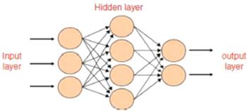
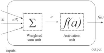
An artificial neural network [13, 14] was utilized to model the impedance and electrical conductivity of phenol red compound. The design of the neural system has a number of layers (input, output, and hidden layers) that involve a number of neurons (see figure 1). The treatment units of the system are the neurons. These neurons are connected to each other in various layers through links called weights, then an activation function is applied to the total of the weighted inputs of each neuron to obtain the neuron's output, see figure 2. An artificial neural network is made using many stages: first, definition of the input and output parameters for training the network; second, validation of the neural network performance to select the best structure; and finally, testing the information which was not already utilized to train the system. A learning algorithm is characterized as a method for modifying the weights and biases of a network to decrease the error function between the network output and the right output already known. The mean squared error (MSE) was determined as [15]:(1)$\begin{eqnarray}{\rm{MSE}}=\displaystyle \frac{\,1}{n}\displaystyle \sum _{i=1}^{n}{({e}_{i})}^{2},\end{eqnarray}$where n is the number of information inputs and ${e}_{i}$ is the difference between the target yield and the system yield.

Figure 1.

New window|Download| PPT slide
Figure 1.The architecture of a multilayer network with one hidden layer of four neurons.

Figure 2.

New window|Download| PPT slide
Figure 2.A simple neuron model: each input X_i is weighted by a factor W_i. The total of all inputs is calculated ${\sum }_{\mathrm{all\; inputs}}{W}_{i}{X}_{i},$ then an activation function f is applied to the product a. The neural result is taken to be f (a); and f (a)=activation function (${\sum }_{\mathrm{all\; inputs}}{W}_{i}{X}_{i}$).

4. Results and discussion

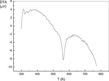
Figure 3 represents the DTA curve for the phenol red in powder form. A sharp endothermic peak was observed at 563 K. Thus, the range of temperatures between room temperature and the determined 563 K is consistent with the electrical measurements of bulk phenol red.

Figure 3.

New window|Download| PPT slide
Figure 3.DTA for powdered phenol red.

4.1. Impedance spectroscopy

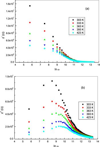
Complex impedance spectroscopy has been extensively applied as a useful tool for examining the frequency-dependent electrical properties of materials [16]. This procedure allows for the separation of the real and imaginary components of the complex impedance and related parameters. It also affords information about the structural properties of the material [17]. Complex impedance (Z*) has two components; Z^/ and Z^//, which are the real and imaginary components of Z*, respectively [17, 18]. The frequency dependence of the real part of the complex impedance (Z^/) for bulk phenol red is shown in figure 4(a) for different temperatures. It can be seen that Z^/ decreases with an increase of frequency, pointing to an increase in conductivity of the sample of phenol red [19]. At lower frequencies and temperatures, the Z^/ curves show a high dispersion with larger values, that indicate larger effects of polarization in the sample. The Z^/ values for different temperatures are then followed by a further decrease until they merge together at high frequencies. This behavior of Z^/ suggests a slow dynamic relaxation process in the phenol red and may be due to the release of space charges [20]. Moreover, at a specific frequency the value of Z^/ decreases with an increase of temperature, indicating a negative temperature coefficient of resistance (NTCR) type of behavior [21]. Figure 4(b) shows the frequency dependence of the imaginary part of the impedance (Z^//) for bulk phenol red at different temperatures. The value of Z^// increases over a range of low frequencies showing a characteristic peak at each temperature. Z^// then decreases with a further increase in frequency. In this way, the nature of Z^// displays the presence a relaxation process in the material. The broadening of the peaks of the Z^// curves signifies the existence of temperature-dependent relaxation phenomena in phenol red [22]. In the high-frequency range, Z^// reduced and amalgamated at all of the temperatures in the study, as a result of the accumulation of space charge in the material [23].

Figure 4.

New window|Download| PPT slide
Figure 4.The frequency dependence of the parts of complex impedance for bulk phenol red at different temperatures: (a) the real part of Z^/, (b) the imaginary part of Z^//.


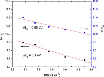
The peak position in the phenol red Z^// curves moved to high-frequency values with increasing temperature. The shift seen in the peak frequency (ω_z) is attributed to the existence of electrical relaxation in phenol red material [24]. The dependence of the frequency (ω_z), of each peak on temperature follows the Arrhenius relation ([25]):(2)$\begin{eqnarray}{\omega }_{{\rm{z}}}=\omega ^{\prime} {{\rm{e}}}^{\left(\tfrac{-{\rm{\Delta }}{E}_{{\rm{z}}}}{kT}\right)},\end{eqnarray}$where ω′ is the pre-exponent factor, k is Boltzmann's constant, T is the absolute temperature and ΔE_z is the activation energy of the relaxation process. The value of ΔE_z (0.1 eV) of bulk phenol red was calculated from the slope of the linear fit for the experimental data points in figure 5.

Figure 5.

New window|Download| PPT slide
Figure 5.The temperature dependence of lnω_z and lnω_M.


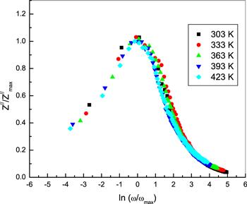
Figure 6 represents the scaling behavior of Z^// at different temperatures for bulk phenol red. All of the values of Z^///Z^//_max for phenol red at different temperatures nearly overlap in one main curve. This is an outcome of the dynamic process of the charge, which, occurring at different time scales, displayed the same activation energy [26]. Thus, the distribution function of the relaxation times is nearly temperature-independent, with non-exponential conductivity relaxation [27].

Figure 6.

New window|Download| PPT slide
Figure 6.The scaling of Z^// spectra for bulk phenol red at different temperatures.


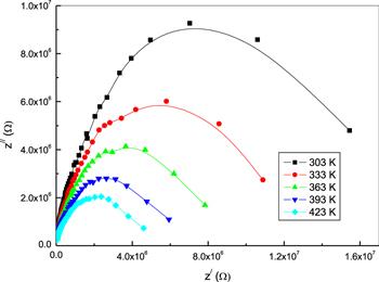
Figure 7 shows Nyquist plots (Z^/ versus Z^//) of bulk phenol red at different temperatures. The plots exhibit semicircle arcs at different temperatures. The effect of temperature on the impedance behavior is much more notable at higher temperatures, as seen from the figure. The single semicircular arc suggests the presence of a granular interior (bulk) property of the material [28]. The area of the semicircle decreases with rising temperature owing to the associated decrease of the impedance. This suggests a temperature dependence on relaxation [22]. Also, the semicircles are shifted to higher frequencies, indicating that the bulk resistance of the Au/phenol red/Au sample decreases with an increase in temperature. This behavior is an indication of a thermally-activated conduction mechanism [29]. Each semicircle arc in the Nyquist plots of phenol red can be represented by an equivalent electrical circuit that consists of a parallel resistor and a capacitor [24], as shown in figure 7. The intercept of the semicircle arc on the Z^/-axis as ω→zero gives the bulk resistance (R) value of the sample [30]. As can be seen from table 1, the values of R decrease with an increase in temperature. This behavior may be attributed to thermal agitation of the charge [31].

Figure 7.

New window|Download| PPT slide
Figure 7.A Nyquist plot of Z^/ versus Z^// for bulk phenol red at different temperatures.



Table 1.
Table 1.Values of resistance for bulk phenol red at different temperatures.

T (K)	303	333	363	393	423
R (MΩ)	18.87	12.97	9.24	6.57	5.35

New window|CSV

4.2. Electrical conductivity

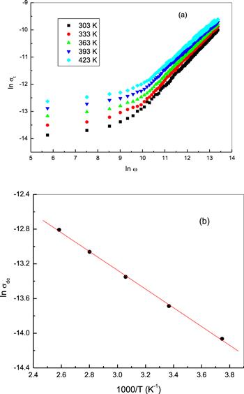
For most solids, the total conductivity (σ_t) can be expressed as [19, 32, 33]:(3)$\begin{eqnarray}{\sigma }_{{\rm{t}}}=G{\omega }^{\eta }+{\sigma }_{{\rm{dc}}},\end{eqnarray}$where Gω^η≡σ_ac (AC conductivity) [34, 35], G is a temperature-dependent but frequency-independent quantity, η is the frequency exponent that takes values between zero and one and σ_dc is DC conductivity. Figure 8(a) represents the frequency dependence of the total conductivity σ_t(ω) for bulk phenol red. As seen from the figure, σ_t of bulk phenol red exhibits a moderate increase in the low-frequency region. It the rises as the frequency increases in the investigated range of temperatures (303-423 K). The σ_dc represents the frequency-independent total conductivity values in the low-frequency range down to zero [36]. The temperature dependence of σ_dc is illustrated in figure 8(b), which shows the Arrhenius-type behavior, that is described by ${\sigma }_{{\rm{dc}}}={\sigma }_{{\rm{o}}}{{\rm{e}}}^{\left(\tfrac{-{\rm{\Delta }}{E}_{{\rm{dc}}}}{kT}\right)}$ [37]. σ_o is a pre-exponential factor and ΔE_dc is the activation energy for DC conduction. The value of ΔE_dc for bulk phenol red was determined to be 0.094 eV. This value is comparable to that observed for the relaxation process ΔE_z. This result may point to that conclusion that the conduction and relaxation phenomena are related to the same origin, i.e. the charge carriers, that have to overcome the same energy barrier for conduction and also relaxation in phenol red [25, 38].

Figure 8.

New window|Download| PPT slide
Figure 8.(a) The frequency dependence of the total electrical conductivity σ_t, for bulk phenol red at different temperatures and (b) the temperature dependence of DC conductivity σ_dc.


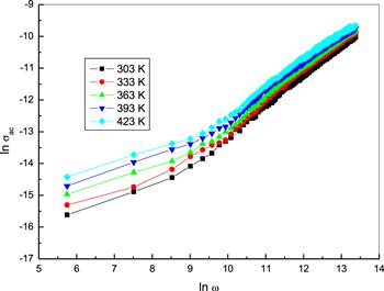
Figure 9 represents the frequency dependence of the AC conductivity, σ_ac(ω) for bulk phenol red pellets at different temperatures. The conductivity showed an increase with a rise in frequency. The exponent frequency η was calculated from the slope of the linear segments of the plots and is shown in figure 10. It diminished as temperature increased. As reported by the models which describe the temperature dependence of the frequency exponent [39], the obtained values for η are in agreement with the correlated barrier hopping (CBH) model. Consequently, the mechanism for AC conduction in bulk phenol red follows the CBH model. According to this model, the frequency exponent, η is expressed as [40]:(4)$\begin{eqnarray}\eta =1-\displaystyle \frac{6kT}{{B}_{{\rm{M}}}-kT\,\mathrm{ln}\left(\tfrac{1}{\omega {\tau }_{o}}\right)},\end{eqnarray}$where B_M is the maximum barrier height of the bulk phenol red and τ_o is the characteristic relaxation time. The frequency exponent could be approximated to the first order by a relation of the form of [41-43]:(5)$\begin{eqnarray}\eta =1-\displaystyle \frac{6kT}{{B}_{{\rm{M}}}}.\end{eqnarray}$

Figure 9.

New window|Download| PPT slide
Figure 9.The frequency dependence of AC electrical conductivity σ_ac, for bulk phenol at different temperatures.

Figure 10.

New window|Download| PPT slide
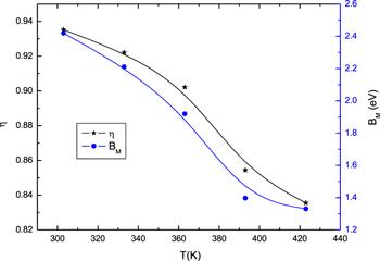
Figure 10.Temperature dependence of the frequency exponent (η) and the maximum barrier height (B_m).


The values of B_M were calculated using equation (6) by substituting the frequency exponent values for different temperatures. The variation of B_M for bulk phenol red against temperature exhibits an analogous decrease with that produced by changing the frequency exponent with temperature as shown in figure 10.

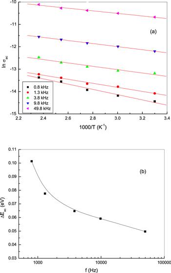
The temperature dependence of the AC conductivity (σ_ac) of bulk phenol red is shown in figure 11(a) at certain frequencies. As can be noticed from the figure, the σ_ac of phenol red increases with increasing temperature. This suggests that σ_ac is a thermally-activated process of an activation energy (ΔE_ac), which was determined using an Arrhenius temperature dependence of σ_ac: σ_ac=σ_o exp (−ΔE_ac/kT). The activation energy for AC conduction was calculated at different frequencies and plotted as a function of frequency, as shown in figure 11(b). The ΔE_ac of phenol red decreases with increasing frequency. A rise of the applied field frequency promotes an electronic jump between the localized states, consequently ΔE_ac decreases with increasing frequency [44]. The smaller values of AC activation energy as compared with that of DC activation energy affirm that hopping conduction is the dominant mechanism for carrier transport between localized states in phenol red [35, 45].

Figure 11.

New window|Download| PPT slide
Figure 11.(a) The temperature dependence of AC electrical conductivity σ_ac, at different frequencies and (b) the variation in ΔE_ac as a function of frequency for bulk phenol.

4.3. Modeling the real and imaginary parts of impedance and total electrical conductivity using ANN

Artificial neural network-based methods have been used in the fields of materials science and engineering research prediction, modeling, control, recognition design, and optimization. The reason for using artificial neural networks for materials science research is their ability to identify and learn the underlying nonlinear relationships between the input and output data. Furthermore, there is a need to recognize the properties of the materials used in design and manufacture, to maximize their capabilities for different applications, both experimentally and theoretically. The application of artificial neural network models in materials science research is becoming increasingly popular and is widely used in various branches of advanced materials science research by many authors [46]. Wang et al [47] established the use of a neural network model to predict the refractive index of ionic liquids and alcohols at different temperatures. Li et al [48] reported on using ANN models to predict the polarizability and the absolute permittivity of hydrocarbon compounds.

4.3.1. The structure of the ANN model

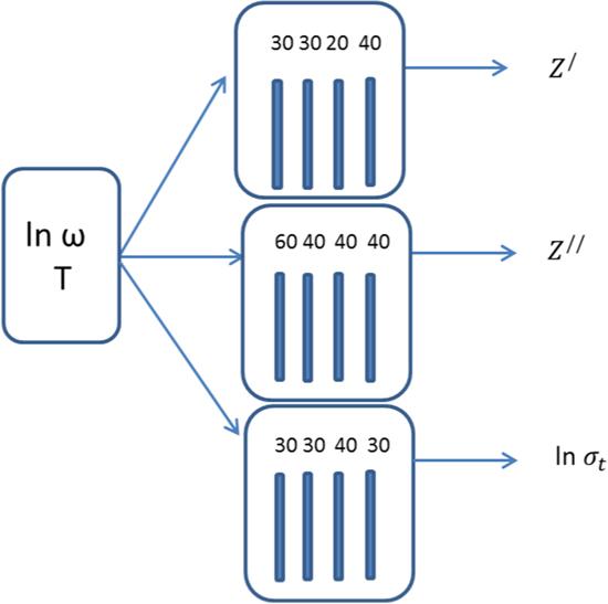
In the present study, an artificial neural network model was used to simulate and predict the impedance and the total electrical conductivity. Using this technique, we attempted to mathematically model the real and imaginary impedance and the total electrical conductivity using ANNs. In this regard, three different ANN models were designed to achieve this goal. The proposed ANN models are presented in figure 12. The first model calculates and predicts the real part of the impedance. The second model simulates and predicts the imaginary part of the impedance and third model calculates and predicts the total electrical conductivity. The parameters used in all three networks are found in table 2.

Figure 12.

New window|Download| PPT slide
Figure 12.A block diagram of ANN-based modeling of Z^/, Z^// and ln σ_t.



Table 2.
Table 2.Overview of all the parameters in the ANNs for Z^/, Z^// and ln σ_t for bulk phenol red.

No.	Structural part of the ANN	ANN1	ANN2	ANN3
1	Inputs	lnω, T	lnω, T	lnω, T
2	Outputs	Z/	Z//	ln σt
3	No. of hidden layers	4	4	4
4	No. of neurons	30, 30, 20, 40	60, 40, 40, 40	30, 30, 40, 30
5	No. of epochs=no. of training	1000	800	1000
6	Training algorithm	trainrp	trainrp	trainrp
7	Performance	0.005	0.026	0.0002
8	Transfer function	logsig	logsig	logsig
9	Output function	purelin	purelin	purelin

New window|CSV

4.3.2. Simulation results

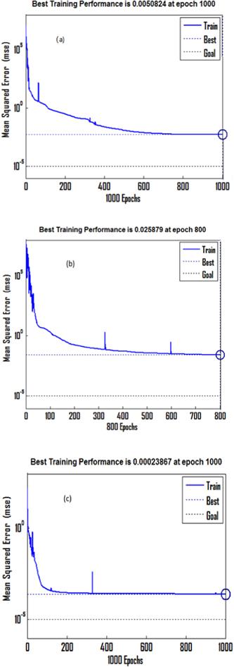
The model was trained using experimental data. The ANN was trained for the measured datasets. The network was exercised to get a better MSE and the best execution for the network. The training techniques are found in figures 13(a)-(c), which reveal the mean squared error of the system beginning at a higher value and decreasing to the smallest one. It appears the network is learning. Training was terminated after an average mean square error of (0.005, 0.026 and 0.0002) was reached for the three (1000, 800 and 1000 Epochs) ANNs, respectively. The performance of the trained network was examined by the relation between the simulated results from the trained neural system and the experimental data (target), see figures 14(a)-(c). A very good coincidence between the model results and the validation data was obtained, which shows that the prepared system has optimal generalization performance. Also, the prediction of the impedance and the total electrical conductivity (at 393 K) which were not included in our training of our model, were found to be in good coincidence with the target. In addition, the equation obtained from our model predicts the impedance and the total electrical conductivity at 443 K, which was not found in training and was predicted by our model alone. Thus, ANN can predict the results of any other temperature, this gives the ANN the possibility for wide utilization in modeling the real and imaginary parts of the impedance and the total electrical conductivity of bulk phenol red.

Figure 13.

New window|Download| PPT slide
Figure 13.The training procedure for ANN models for (a) Z^/, (b) Z^// and (c) ln σ_t at different temperatures.

Figure 14.

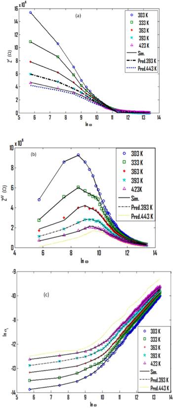New window|Download| PPT slide
Figure 14.The ANN simulation and prediction results for (a) Z^/, (b) Z^// and (c) ln σ_t at different temperatures.

4.4. The electric modulus formalism

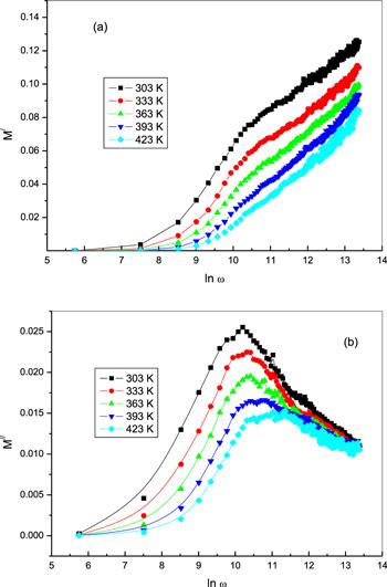
Modulus spectroscopy expounds the bulk dielectric behavior of materials and this formalism diminishes the effects of electrode polarization [49, 50]. The electric modulus (M*) of a material is calculated as [51, 52]:(6)$\begin{eqnarray}{M}^{* }\left(\omega \right)={M}^{/}\left(\omega \right)+{\rm{j}}{M}^{//}\left(\omega \right),\end{eqnarray}$where M^/(ω) and M^//(ω) are the real and imaginary parts of the electrical modulus, respectively. Figures 15(a) and (b) show the variation of M^/(ω) and M^//(ω) spectra as a function of frequency for bulk phenol red over a range of temperatures (303-423 K). The M^/ of bulk phenol red shows an increase with rising frequency at different temperatures. The spectra of M^/ show a long tail at low frequencies, implying that a large capacitance is associated with the interface [53] between the electrode and the phenol red sample. The variation of M^// as a function of frequency in figure 15(b) displays a single relaxation peak. Its position is transferred to a high frequency with rising temperature. The charge carrier movement becomes quicker as the temperature is elevated. This leads to a reduction in the time of relaxation and a consequent movement in the peak position of M^// towards higher frequencies. This behavior suggests the presence of a temperature-dependent hopping mechanism for AC electrical conduction [54]. The ω_M corresponding to the frequency at the maximum value of M^// is plotted as a function of temperature, as shown in figure 5. The relation thus obtained obeys Arrhenius' law with an activation energy of ΔE_M. Using a linear-fit analysis for the data in figure 5, ΔE_M was calculated to be 0.08 eV and that value is close to the activation energy obtained for Z^// i.e. (ΔE_z). This suggests that the relaxation and conduction processes may be attributed to the same type of charge carriers [26]. Figure 16 shows the frequency dependence of normalized functions Z^///Z^//_max and M^///M^//_max at 303 K (as a representative example). The non-overlap for the peaks suggests a non-Debye-type relaxation process for the phenol red material [54].

Figure 15.

New window|Download| PPT slide
Figure 15.The frequency dependence of (a) the real part of the electric modulus M^/, and (b) the imaginary part of the electric modulus M^// for bulk phenol at different temperatures.

Figure 16.

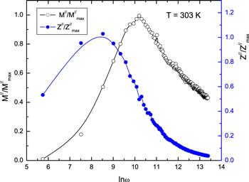New window|Download| PPT slide
Figure 16.The normalized spectra of Z^///Z^//_max and M^///M^//_max as a function of frequency at 303 K.

5. Conclusions

The electrical and dielectric behavior of bulk phenol red were investigated by studying complex impedance and modulus spectroscopy. Z^/ (the real part of the complex impedance) of phenol red decreases with an increase of temperature, expressing a negative temperature coefficient of resistance type of behavior. The behavior of Z^// (the imaginary part of the complex impedance) of phenol red exhibited the existence of a relaxation process in the material with an activation energy of 0.1 eV. The peaks of the Z^// spectra were shifted to a higher frequency on increasing temperature. The scaling behavior of Z^// at specific temperatures for bulk phenol red suggests that the dynamic charge processes occurring at different time scales displayed the same activation energy. Nyquist plots (Z^/ versus Z^//) of bulk phenol red exhibited semicircle arcs. The variation of the DC conductivity with temperature showed an Arrhenius relation dependence with an activation energy of 0.094 eV. The AC electrical conductivity obeyed a universal power law with a frequency exponent decreasing with a rising temperature and satisfied the correlated barrier hopping model. The barrier height displayed a similar nature for the frequency exponent in its dependence on temperature. In the imaginary part of the spectra of the electric modulus, a single relaxation peak was noticed and its position shifted to a high frequency with rising temperature. The activation energy estimated for M^// was close to the activation energy obtained for Z^//. The frequency reliance of the normalized functions Z^///Z^//_max and M^///M^//_max and suggests a non-Debye-type relaxation process for the phenol red material. Moreover, a four-layer feed neural network was optimized to predict the real and imaginary parts of the impedance and the electrical conductivity of bulk phenol red at certain temperatures. The lowest MSE values were found (0.005, 0.026 and 0.0002) with four hidden layers. A regression analysis was performed between the model's predicted values and the experimental results. The ANN-predicted values are in close agreement with those determined from experimental results in the simulation and prediction process. Thus, the ANN model can effectively simulate and predict the electrical properties of bulk phenol red.

Acknowledgments

The authors are grateful to Prof. M M El-Nahass, Ain Shams University, for his fruitful discussions.

Reference View Option By original order
By published year
By cited within times
By Impact factor

[1]Sun S-S Dalton L R 2008 Introduction to Organic Electronics and Optoelectronics Materials and Devices Boca Raton, FL CRC Press
[Cited within: 1]

[2]Wilbers J G E Xu B Bobbert P A de Jong M P van der Wiel W G 2017 Sci. Rep. 7 41171
DOI:10.1038/srep41171 [Cited within: 2]

[3]Świst A Soloducho J 2012 Chemik 66 289
[Cited within: 1]

[4]Alias A N Zabidi Z M Ali A M M Harun M K Yahya M Z A 2013 Int. J. Appl. Sci. Technol. 3 11
[Cited within: 1]

[5]Blanche P-A 2016 Photorefractive Organic Materials and Applications Springer Series in Materials Science vol 240 Berlin Springer 65
[Cited within: 2]

[6]Coropceanu V Cornil J da Silva Filho D A Olivier Y Silbey R Bréda J L 2007 Chem. Rev. 107 926
DOI:10.1021/cr050140x [Cited within: 1]

[7]Li L Winckel S V Genoe J Heremans P 2009 Appl. Phys. Lett. 95 153301
DOI:10.1063/1.3246160 [Cited within: 1]

[8]Karthikeyan P Thamizhendhi G 2016 Int. J. Emerg. Trends Eng. Dev. 4 67
[Cited within: 1]

[9]Asadi-Eydivand M Solati-Hashjin M Farzadi A Abu Osman N A 2014 Ceram. Int. 40 12439
DOI:10.1016/j.ceramint.2014.04.095 [Cited within: 2]

[10]Paliwal M Kumar U A 2009 Expert Syst. Appl. 36 2
DOI:10.1016/j.eswa.2007.10.005

[11]Haykin S 2004 Neural Netw. 2 23
[Cited within: 1]

[12]Ali H A M 2017 Eur. Phys. J. Plus 132 327
DOI:10.1140/epjp/i2017-11595-4 [Cited within: 1]

[13]Esfe M H Saedodin S Bahiraei M Toghraie D Mahian O Wongwises S 2014 J. Therm. Anal. Calorim. 118 287
DOI:10.1007/s10973-014-4002-1 [Cited within: 1]

[14]Mohd Noor C W Mamat R Najafi G Wan Nik W B Fadhi M 2015 Mater. Sci. Eng. 100 012023
DOI:10.1088/1757-899X/100/1/012023 [Cited within: 1]

[15]Esfe M H Rostamian H Afrand M Karimipour A Hassani M 2015 Int. Commun. Heat Mass Transfer 68 98
DOI:10.1016/j.icheatmasstransfer.2015.08.015 [Cited within: 1]

[16]Lee J H Chou H Wen G H Hwang G H 2010 J. Appl. Phys. 107 023907
DOI:10.1063/1.3273319 [Cited within: 1]

[17]Barik S K Choudhary R N P Singh A K 2011 Adv. Mat. Lett. 2 419
DOI:10.5185/amlett.2011.2228 [Cited within: 2]

[18]Mudenda S Kale G M 2015 J. Mater. Chem. A 3 12268
DOI:10.1039/C5TA01660F [Cited within: 1]

[19]Thomas A K Abraham K Thomas J Saban K V 2017 J. Asian Ceram. Soc. 5 56
DOI:10.1016/j.jascer.2017.01.002 [Cited within: 2]

[20]Lily Kumari K Prasad K Choudhary R N P 2008 J. Alloys Compd. 453 325
DOI:10.1016/j.jallcom.2006.11.081 [Cited within: 1]

[21]Kaushal A Olhero S M Singh B Fagg D P Bdikin I Ferreira J M F 2014 Ceram. Int. 40 10593
DOI:10.1016/j.ceramint.2014.03.038 [Cited within: 1]

[22]Das P S Chakraborty P K Behera B Mohanty N K Choudhary R N P 2014 J. Adv. Ceram. 3 1
DOI:10.1007/s40145-014-0087-z [Cited within: 2]

[23]Das P R Pati B Sutar B C Choudhury R N P 2012 J. Mod. Phys. 3 870
DOI:10.4236/jmp.2012.38114 [Cited within: 1]

[24]Rosaiah P Hussain O M 2013 Int. J. Mod Phys: Conf. Ser. 22 517
DOI:10.1142/S201019451301060X [Cited within: 2]

[25]Khiar A S A Puteh R Arof A K 2006 Physica B 373 23
DOI:10.1016/j.physb.2005.10.104 [Cited within: 2]

[26]Tang R Jiang C Qian W Jian J Zhang X Wang H Yang H 2015 Sci. Rep. 5 13645
DOI:10.1038/srep13645 [Cited within: 2]

[27]Badapanda T Harichandan R K Nayak S S Mishra A Anwar S 2014 Process. Appl. Ceram. 8 145
DOI:10.2298/PAC1403145B [Cited within: 1]

[28]Khatri P Behera B Srinivas V Choudhary R N P 2008 Res. Lett. Mater. Sci. 2008 746256
DOI:10.1155/2008/746256 [Cited within: 1]

[29]Padmasree K P Kanchan D K Kulkarni A R 2006 Solid State Ionics 177 475
DOI:10.1016/j.ssi.2005.12.019 [Cited within: 1]

[30]Padmamalini N Ambujam K 2016 Karbala Int. J. Modern Sci. 2 271
DOI:10.1016/j.kijoms.2016.10.001 [Cited within: 1]

[31]Song C H Kim M Lee S M Choi H W Yang Y S 2010 J. Korean Phys. Soc. 56 462
DOI:10.3938/jkps.56.462 [Cited within: 1]

[32]Elliott S R 1987 Adv. Phys. 36 135
DOI:10.1080/00018738700101971 [Cited within: 1]

[33]Jonscher A K 1977 Nature 267 673
DOI:10.1038/267673a0 [Cited within: 1]

[34]Sharma A Mehta N Kumar A 2011 J. Mater. Sci. 46 4509
DOI:10.1007/s10853-011-5344-8 [Cited within: 1]

[35]Nermec P Frumar M Frumarova B Jelinek M Lancok J Jedelsky J 2000 Opt. Mater. 15 191
DOI:10.1016/S0925-3467(00)00035-5 [Cited within: 2]

[36]El-Nahass M M Ali H A M 2012 Solid State Commun. 152 1084
DOI:10.1016/j.ssc.2012.03.002 [Cited within: 1]

[37]Ali A A Shaaban M H 2011 Bull. Mater. Sci. 34 491
DOI:10.1007/s12034-011-0103-7 [Cited within: 1]

[38]Smari M Rahmouni H Elghoul N Walha I Dhahri E Khirouni K 2015 RSC Adv. 5 2177
DOI:10.1039/C4RA11323C [Cited within: 1]

[39]El-Nahass M M Farid A M Amer H H Abdel-Rahman K F Ali H A M 2008 Physica B 403 2331
DOI:10.1016/j.physb.2007.12.015 [Cited within: 1]

[40]Velayutham T S Abd Majid W H Gan W C Khorsand Zak A Gan S N 2012 J. Appl. Phys. 112 054106
DOI:10.1063/1.4749414 [Cited within: 1]

[41]Pike G E 1972 Phys. Rev. B 6 1572
DOI:10.1103/PhysRevB.6.1572 [Cited within: 1]

[42]Amer N M Saleh A M Gould R D 2003 Appl. Phys. A 76 77
DOI:10.1007/s003390201306

[43]Abu-Hilal A O Gould R D Abu-Taha M I Saleh A M 2007 Int. J. Mod. Phys. B 21 55
DOI:10.1142/S021797920703587X [Cited within: 1]

[44]Ali H A M Soliman H S Saadeldin M Sawaby K 2014 Mater. Sci. Semicond. Process. 18 141
DOI:10.1016/j.mssp.2013.11.006 [Cited within: 1]

[45]Ebnalwaled A A 2010 Mater. Sci. Eng. B 174 285
DOI:10.1016/j.mseb.2010.03.029 [Cited within: 1]

[46]Singh M Kaur H 2016 Curr. Rep. Sci. Tech. 2 145
[Cited within: 1]

[47]Wang N Yang Z Li Y 2019 Energy Sources A 26 1 10
DOI:10.1080/15567036.2019.1648605 [Cited within: 1]

[48]Li H Liu X Yang S Yi T Yang Z Yuan W 2014 Int. J. Electrochem. Sci. 9 3725
[Cited within: 1]

[49]Ravi M Pavani Y Kiran Kumar K Bhavani S Sharma A K Narasimha Rao V V R 2011 Mater. Chem. Phys. 130 442
DOI:10.1016/j.matchemphys.2011.07.006 [Cited within: 1]

[50]Mogusˇ-Milankovic´ A Pavic L Srilatha K Srinivasa Rao C Srikumar T Gandhi Y Veeraiah N 2012 J. Appl. Phys. 111 013714
DOI:10.1063/1.3676254 [Cited within: 1]

[51]El Hasnaoui M Graça M P F Achour M E Costa L C 2011 Mater. Sci. Appl. 2 1421
DOI:10.4236/msa.2011.210192 [Cited within: 1]

[52]Mahamoud H Louati B Hlel F Guidara K 2011 Bull. Mater. Sci. 34 1069
DOI:10.1007/s12034-011-0163-8 [Cited within: 1]

[53]Pal P Ghosh A 2017 J. Appl. Phys. 122 015101
DOI:10.1063/1.4991484 [Cited within: 1]

[54]Hossen M B Akther Hossain A K M 2015 J. Adv. Ceram. 4 217
DOI:10.1007/s40145-015-0152-2 [Cited within: 2]