Yao Ma^,1, Wen-Qi Niu^,1, Yu-Fei Wang^,2,∗, Han-Qing Zheng^,1,31Department of Physics and State Key Laboratory of Nuclear Physics and Technology, Peking University, Beijing 100871, China
²Helmholtz Institut für Strahlen- und Kernphysik, University of Bonn, Bonn D-53115, Germany
³Collaborative Innovation Center of Quantum Matter, Beijing, China

First author contact: ∗ Author to whom any correspondence should be addressed.
Received:2020-05-16Revised:2020-06-19Accepted:2020-06-22Online:2020-09-29


Abstract
We give a pedagogical analysis on K-matrix models describing the πN scattering amplitude, in S₁₁ channel at low energies. We show how the correct use of analyticity in the s-channel and crossing symmetry in t- and u-channels leads to a much improved analytic behavior in the negative s region, in agreement with the prediction from chiral perturbation amplitudes in its validity region. The analysis leads again to the conclusion that a genuine N*(890) resonance exists.
Keywords： pi N scattering;subthreshold pole;K-matrix;N*(890)


PDF (474KB)MetadataMetricsRelated articlesExportEndNote|Ris|BibtexFavorite
Cite this article
Yao Ma, Wen-Qi Niu, Yu-Fei Wang, Han-Qing Zheng. How does the S₁₁N*(890) state emerge from a naive K-matrix fit?. Communications in Theoretical Physics, 2020, 72(10): 105203- doi:10.1088/1572-9494/aba25d

In a series of recent publications [1-3], it is suggested that there exists a subthreshold resonance in the S₁₁ channel of πN scattering, with $M-{\rm{i}}{\rm{\Gamma }}/2=895(81)-{\rm{i}}164(23)$ MeV. The result is completely novel and is obtained based on an approach([4-6]) with full respects to fundamental principals of S-matrix theory such as unitarity, analyticity and consistent with crossing symmetry([7, 8]). The approach is much superior to conventional unitarization approximations, such as K-matrix method or variations of Padé approximation (for the discussion, see for example [9, 10]).

Specifically, in the regime of Peking University (PKU) representation [1-3], input the left-hand cut from chiral perturbation theory results, while the inelasticity and known poles are fixed from experimental data. Due to the negative definite contributions from left-hand cut to the phase shift, and positive definite contributions from known resonances and inelasticity, we claim that a subthreshold resonance must exist, irrespective to the details of calculations, in S₁₁ channel. Especially [3], gives a comprehensive analysis on not only the N*(890) pole but also the physics of all other S- and P-wave channels.

Nevertheless, those works have still received some queries: firstly, why do many previous works do not find significant effects from N*(890) resonance? Secondly [1-3], inputs the left-hand cut only from chiral perturbation theory, which may not work well in the region far away from threshold.

The aim of this paper is to make a further analysis in the conventional K-matrix approach, to examine and to understand why the N*(890) was missed in previous researches, and how it can appear even in a simple K-matrix analysis, if one be respectful to the analyticity property of scattering amplitude offered by standard quantum field theory. We hope the analysis made in this paper be helpful to convince the physics community to accept the existence of the N*(890) resonance.

To begin with, let us start from the standard coupled channel K-matrix formula:(1)$\begin{eqnarray}{T}^{-1}={K}^{-1}-{\rm{i}}\rho ,\end{eqnarray}$where ρ is a diagonal matrix with its elements being the kinematical factors in each channel, i.e. $\rho ={\rm{diag}}({\rho }_{1},{\rho }_{2})$. To be specific, the subscripts 1, 2 means πN and ηN channels, respectively. Hence(2)$\begin{eqnarray}\begin{array}{rcl}{\rho }_{1} & = & \sqrt{\left[s-{\left({m}_{N}+{m}_{\pi }\right)}^{2}\right]\left[s-{\left({m}_{N}-{m}_{\pi }\right)}^{2}\right]}/s,\\ {\rho }_{2} & = & \sqrt{\left[s-{\left({m}_{N}+{m}_{\eta }\right)}^{2}\right]\left[s-{\left({m}_{N}-{m}_{\eta }\right)}^{2}\right]}/s.\end{array}\end{eqnarray}$

Basically the only requirement on K is that it is a real symmetric matrix in the physical region in order to fulfill unitarity. Hence we start from a simple form (herewith we call it Fit I):(3)$\begin{eqnarray}{K}_{{ij}}=\displaystyle \sum _{\alpha =1,2}\displaystyle \frac{{c}_{{ij}}^{\alpha }}{s-{M}_{\alpha }^{2}}+{P}_{{ij}}^{(2)}(s).\end{eqnarray}$In the above parameterization we put two bare poles with masses M₁ and M₂ because we knew that there are two well established resonance N*(1535) and N*(1650) to be adjusted, in S₁₁ channel; and ${P}_{{ij}}^{(2)}(s)$ are 2nd order real polynomials to simulate the background, and are symmetric in subscripts i and j (so are the coefficients ${c}_{{ij}}^{\alpha }$).

Using equation (3) we fit S₁₁ partial wave data of πN scatterings from threshold upto $\sqrt{s}=2.1$ GeV provided by [11]; and to constrain the near-threshold behavior, we also fit the data of low-energy region in [12] simultaneously. The fit is plotted in figure 1. In practice, the K-matrix fit is notoriously known as producing spurious physical sheet resonance poles, but when they (and normal poles) are of less significance, i.e. contributing to the phase shift tinily, people do not care about them. The poles found from Fit I are listed in table 1. Besides, the scattering length is $a\simeq 162.43\times {10}^{-3}{m}_{\pi }^{-1}$, which is compatible with, e.g. the result of Roy-Steiner analyzes in [12]: $a\simeq 169.9(19.4)\times {10}^{-3}{m}_{\pi }^{-1}$.

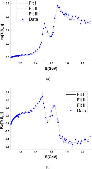
Figure 1.

New window|Download| PPT slide
Figure 1.Fit of GWU data upto $\sqrt{s}=2.1$ GeV, (a) $\mathrm{Im}T$, (b) $\mathrm{Re}T$. Fit I: solid line (black); Fit II: dotted-dashed line (red); Fit III: dashed line (green).



Table 1.
Table 1.Fit I: poles obtained using equation (3).

Sheets	Pole positions on $\sqrt{s}$ plane in unit of GeV
I	1.36 − 0.65i
II	1.68 − 0.07i; 0.73 − 0.19i
III	1.68 − 0.07i; 0.92
IV	1.529 − 0.016i

New window|CSV

Table 1 may deserve a few words of explanation: experienced readers will quickly recognize that poles $1.68-{\rm{i}}0.07$(II) and $1.68-{\rm{i}}0.07$(III) are of N*(1650), whereas $1.529-{\rm{i}}0.016$(IV) and 0.92(III) are of N*(1535) since, as is well known, the former mainly couples to πN while the latter mainly couples to ηN. Though their pole locations may be rather poorly determined, the main interests here is however to investigate the N*(890) pole. Hence we actually do not pay much attention to these well established resonances. Similar to [1-3], in figure 2 phase shifts contributed from different sources are plotted using PKU representation; their sum equals to the fit curve or experimental data, as it should.

Figure 2.

New window|Download| PPT slide
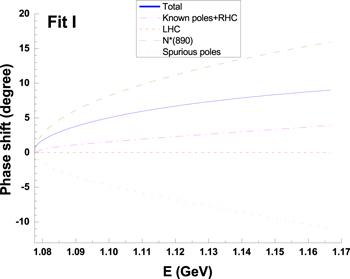
Figure 2.Fit I: different contributions to the phase shift near πN threshold.


We summarize major outputs from Fit I:• The known poles and right hand inelastic cut which begins at the ηN threshold cannot fit the phase shift data. That indicates missing contributions from other sources have to exist.
• The left-hand cut contribution is nearly zero, which is of course not correct as will be discussed at some lengths below.
• Below πN threshold there exists a resonance pole providing a large positive phase shift. Meanwhile a spurious pole on first sheet provides a negative phase shift.


One great advantage of the PKU representation is that different contributions to the phase shift are separable and additive, hence one can calculate different contributions to the phase shift, especially that from the background term in πN channel, $f(s)\equiv \tfrac{\mathrm{ln}{S}_{11}(s^{\prime} )}{2{\rm{i}}{\rho }_{1}(s^{\prime} )}$, with ${S}_{11}\equiv 1+2{\rm{i}}{\rho }_{1}{T}_{11}$:⁴(⁴ For more discussions on related topics, one is referred to [1-3].)(4)$\begin{eqnarray}f(s)=\displaystyle \frac{s}{\pi }{\int }_{L}{\rm{d}}s^{\prime} \displaystyle \frac{\mathrm{Im}(\tfrac{\mathrm{ln}{S}_{11}(s^{\prime} )}{2{\rm{i}}{\rho }_{1}(s^{\prime} )})}{s^{\prime} (s^{\prime} -s)}.\end{eqnarray}$The spectral function in above integral, $\mathrm{Im}f(s^{\prime} )\,=\mathrm{Im}(\tfrac{\mathrm{ln}{S}_{11}(s^{\prime} )}{2{\rm{i}}{\rho }_{1}(s^{\prime} )})$ read off from Fit I is plotted in figure 3. In the non-relativistic limit, function ${\rho }_{1}(s)f(s)$ reduces to $-{kR}$ [13] (see the discussion in [3]) with k the center of mass momentum, and $R=\tfrac{-2f({s}_{R})}{({m}_{\pi }+{m}_{N})}$ where ${s}_{R}={({m}_{\pi }+{m}_{N})}^{2}$ being the physical πN threshold. Naturally, one expects R being the interaction range [14], i.e. $R\simeq 0.52{m}_{\pi }^{-1}\simeq 0.79$ fm for πN scatterings [3]. Notice that with equation (4) we can actually define different contribution from different energy region to the background term, through dividing the integral interval. For example, by calculating ${f}^{\chi {PT}}(s)\propto {\int }_{-{{\rm{\Lambda }}}_{\chi {PT}}^{2}}^{{s}_{L}}$, we may estimate the contribution from the energy region calculable using perturbation theory [15-19]: if ${{\rm{\Lambda }}}_{\chi {PT}}^{2}$ is set as 0.08 GeV² according to the ${N}^{* }(1440)$ pole location [3], then ${R}_{\chi {PT}}=0.39$ fm⁵(⁵ As already discussed in [3], ${{\rm{\Lambda }}}_{\chi {PT}}^{2}=0.08$ GeV² is a bit too optimistic, however the fit requires a larger R value.).

Figure 3.

New window|Download| PPT slide
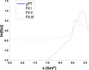
Figure 3.Different estimations on the spectral function of left-hand integral: the solid (blue) line depicts the $\chi {PT}$ result at $O({p}^{3})$ [3]; the dotted straight line (orange) is from Fit I; dotted-dashed (green) line is from Fit II; dashed (green) line is generated by Fit III. Small fluctuations in these curves are either from nearby (spurious) singularities or from numerical instabilities and should be ignored.


It is actually easy to understand why R becomes too small in Fit I. Since the only source of branch point singularity in S₁₁ before the inelastic effect in ρ₂ is switched on, is ${\rm{i}}{\rho }_{1}(s)$, and remember that on the left cut ${\rm{i}}{\rho }_{1}(s+{\rm{i}}\epsilon )=-{\rm{i}}{\rho }_{1}(s-{\rm{i}}\epsilon )$, the S-matrix constructed as such is also unitary on the left! Hence the spectral function of the left-hand integral vanishes. This annoying property of S is due to the over-simplification of equations (1), (3): according to Cutkosky rule, the function iρ(s) comes from the absorptive part of two body intermediate states, thus it should have come along with its dispersive or real part missed in equation (3), which is widely used in the literature. Therefore to cure the deficiency one substitutes iρ(s) in those equations by the well known two point function (also known as Chew-Mandelstam function) ${B}_{0}(s;{m}_{1}^{2},{m}_{2}^{2})$ defined as following (b₀ is a subtraction constant),(5)$\begin{eqnarray}{B}_{0}(s;{m}_{1}^{2},{m}_{2}^{2})={b}_{0}+\displaystyle \frac{s}{\pi }\int {\rm{d}}s^{\prime} \displaystyle \frac{\rho (s^{\prime} )}{s^{\prime} (s^{\prime} -s)}.\end{eqnarray}$

Fit II:

As discussed above, the vanishing of the left-hand cut contribution comes from a poor approximation (on-shell approximation). In order to parameterize the amplitude with better analyticity property, one should at least pick up the dispersive part together with the absorptive part. From equation (5), it reads as, upto a subtraction constant,(6)$\begin{eqnarray}\begin{array}{rcl}{B}_{0}(s,{m}_{1}^{2},{m}_{2}^{2}) & = & \displaystyle \frac{1}{\pi }+\displaystyle \frac{1}{2\pi s}\left\{[s(1+\rho (s))\right.\\ & & -\,{\rm{\Delta }}]\mathrm{ln}[\displaystyle \frac{{\rm{\Delta }}+s(1-\rho (s))}{{\rm{\Delta }}-s(1+\rho (s))}]\\ & & +\,[s(1-\rho (s))-{\rm{\Delta }}]\\ & & \times \ \mathrm{ln}\left[\displaystyle \frac{{\rm{\Delta }}+s(1+\rho (s))}{{\rm{\Delta }}-s(1-\rho (s))}\right]\},\end{array}\end{eqnarray}$where ${\rm{\Delta }}={m}_{N}^{2}-{m}_{\pi }^{2}$ for example. This function has the same imaginary part as iρ(s) in the physical region, but maintains quite different analyticity property: it is analytic on the left while iρ(s) contains a left cut starting from ${s}_{L}={({m}_{N}-{m}_{\pi })}^{2}$ to $-\infty $.

We therefore unitarize the amplitude in the following way:(7)$\begin{eqnarray}\begin{array}{rcl}{T}^{-1} & = & {K}^{-1}-B,\\ B & \equiv & \mathrm{diag}\{{B}_{0}(s,{m}_{\pi }^{2},{m}_{N}^{2}),{B}_{0}(s,{m}_{\eta }^{2},{m}_{N}^{2})\},\end{array}\end{eqnarray}$and parameterize the K-matrix as before, and fit data of πN scattering amplitude from threshold to 2.1 GeV. The fit is also plotted in figure 1.

Nearby poles found from Fit II are listed in table 2. We also plot $\mathrm{Im}(\tfrac{\mathrm{ln}{S}_{11}(s^{\prime} )}{2{\rm{i}}{\rho }_{1}(s^{\prime} )})$ read off from Fit II in figure 3. The scattering length does not change much: $a\simeq 164.11\times {10}^{-3}{m}_{\pi }^{-1}$. We find significant improvement on the left-hand cut. It has now a similar behavior with the $\chi {PT}$ calculation in the validity region of the latter, meanwhile contributes still negatively to the integral of f defined in equation (4): in the region from 0 to ${s}_{L}={({m}_{N}-{m}_{\pi })}^{2}$, the function $\mathrm{Im}(\tfrac{\mathrm{ln}{S}_{11}(s^{\prime} )}{2{\rm{i}}{\rho }_{1}(s^{\prime} )})$ is positive definite and $\tfrac{1}{s^{\prime} (s^{\prime} -s)}$ is negative, hence according to equation (4), the contribution to the integral in this region is negative; while in the region from $-\infty $ to 0, $\mathrm{Im}(\tfrac{\mathrm{ln}{S}_{11}(s^{\prime} )}{2{\rm{i}}{\rho }_{1}(s^{\prime} )})$ is negative and $\tfrac{1}{s^{\prime} (s^{\prime} -s)}$ is positive. One gets R=0.18 fm in Fit II which is not as large as what is required by fit [3], but is much improved comparing with the R(=0) value in Fit I. Also, there is an overall improvement of fit quality comparing with that of Fit I, in the sense that the spurious pole is pushed further away as its contribution to the phase shift gets much smaller, as can be seen by comparing figures 2 and 4.

Figure 4.

New window|Download| PPT slide
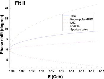
Figure 4.Different contributions to the phase shift in Fit II.



Table 2.
Table 2.Fit II: poles obtained using equation (7).

Sheets	Pole positions on $\sqrt{s}$ plane in unit of GeV
I	1.85 − 0.29i
II	1.66 − 0.04i; 0.77 − 0.23i
III	1.66 − 0.06i; 1.50 − 0.05i
IV	1.53 − 0.01i

New window|CSV

Comparing Fit II with Fit I we observe that the correct use of analyticity in the s-channel, by recovering the dispersive part of the kinematic factor, leads to much improved predictions on the left cuts, the much suppressed spurious pole contribution, and stronger evidence for the existence of N*(890). Inspired by this, one wonder whether the inclusion of t-channel and u-channel cuts could further improve the fit results. We do this in the following Fit III.

Fit III:

We add in the K-matrix the tree diagram contribution of t-channel ρ meson and u-channel nucleon exchanges (though the latter's effect is very small). It now reads,(8)$\begin{eqnarray}{K}_{{ij}}=\displaystyle \sum _{\alpha =1,2}\displaystyle \frac{{c}_{{ij}}^{\alpha }}{s-{M}_{\alpha }^{2}}+{P}_{{ij}}^{(2)}(s)+{K}_{{ij}}^{t,u \mbox{-} {\rm{channel}}},\end{eqnarray}$and T-matrix parameterized as equation (7). Now the ‘left' cut becomes rather complicated, see figure 5. We leave the explanation in the appendix. Fit results are again plotted in figure 1. Nearby poles on four sheets are shown in table 3. The scattering length still does not change much: $a\simeq 167.08\times {10}^{-3}{m}_{\pi }^{-1}$.

Figure 5.

New window|Download| PPT slide
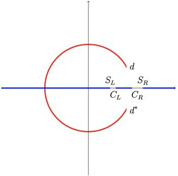
Figure 5.The left cut caused by t-channel ρ meson exchange (circular arc); u-channel exchange (line segment from c_L to c_R [3]).

Figure 6.

New window|Download| PPT slide
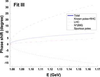
Figure 6.Fit III: the phase shift near πN threshold.



Table 3.
Table 3.Fit III: poles obtained using equation (8).

Sheets	Pole positions on $\sqrt{s}$ plane in unit of GeV
I	1.35 − 0.58i
II	1.67 − 0.07i; 0.93 − 0.27i
III	1.65 − 0.09i; 1.53 − 0.07i
IV	1.54 − 0.01i

New window|CSV

The spectral function read off from Fit III is plotted in figure 3. It is seen that the value of the spectral function now gets more closed to the result in [3], comparing with the Fit II solution in the small $| s| $ region, in the sense that it also produces the circular cut. It is even more important to stress that, the investigation here further justifies the strategy adopted in [1-3], i.e. to use a cut-off parameter to regulate the ‘resonance region' contribution to f(s). Since the ‘resonance region' contribution gives the same sign as comparing with that from perturbation region, the strategy taken in [1-3] will not be bad, as the fit decides the cut-off parameter and, after all, the location of the N*(890) pole will not be annoyed much by such an uncertainty. Numerically, here we obtain $R(\mathrm{left}\,\mathrm{cut})\simeq 0.25\,{\rm{fm}}$, $R(\mathrm{circular}\,\mathrm{arc})\simeq 0.10\,{\rm{fm}}$, their sum is closer to the fit value obtained in [3]. Also, the resonance pole below threshold provides a larger phase shift, see figure 6. Nevertheless the contribution of spurious pole is not found to be further suppressed comparing with Fit II.

At last one would like to fit the data by getting rid of spurious poles and by borrowing the left cuts (both the cut $(-\infty ,{s}_{L}]$ and the circular arc), i.e. to use predictions on ‘left-hand cuts' as an input in applying the PKU representation. The fit to the data is achieved without the need of any spurious poles and cut-off parameters. In this way one gets the subthreshold pole located at $\sqrt{s}\simeq 796(2)-109(8){\rm{i}}$ MeV—a result compatible with the results of [2, 3], even though the R value used here is only half of the value as estimated in [3]. Note that the location of N*(890) pole here numerically may not be necessarily better than the result in [3]; actually the aim of this paper is to show in another way that the strategy of [3] and the existence of N*(890), are reasonable.

To summarize, using a simple unitarization model, in this paper we have shown that, a better treatment of analyticity in the s channel dynamics has led to much improved analytic property on the left side. The inclusion of crossing symmetry, i.e. t- and u-channel resonance exchanges has further improved the quality of its predictions, in the sense that the results get closer to the $\chi {PT}$ ones in the validity region of the latter, as well as the emergence of the circular cut. Using the ‘best' model predictions on the left cuts (i.e. Fit III), one gets the pole location of the N*(890) being consistent with that of [1-3]. And the advantage now is the elimination of any cut-off dependence when evaluating left cut integrals. We think it is important to stress that all the pseudo-thresholds, i.e. ${({m}_{1}-{m}_{2})}^{2}$ are essentially due to relativistic effects and should not be ignored. In a non-relativistic theory, one may take these effects into account through introducing a sizable, physical, and negative background contribution to the phase shift [14].

We notice that in a paper by Döring and Nakayama [20] (see also [21]), the authors found a subthreshold pole at $\sqrt{s}\simeq 1031-203{\rm{i}}$ MeV in S₁₁ channel, without further information on left cuts and spurious poles. The authors carefully quote: However, it is not clear if this state is genuine or a forced pole that mocks up the u- and t-channel subthreshold cuts that are not explicitly included in the present model. The investigations of this paper and [1-3] made it clear, we think, that the subthreshold resonance does not play a role of mocking up the crossed channels effects. The fact is just on the contrary—the former contributes a positive definite phase shift to counter balance the effects of the latter. We have actually witnessed similar things that happened in $\pi \pi $ scatterings and $\pi K$ scatterings, in most attractive channels [4-6, 22].

Acknowledgments

This work is supported in part by the National Nature Science Foundations of China under contract numbers 11975028 and 10925522, and by the Sino-German CRC 110 (Grant No. TRR110). The authors would like to thank Ulf-GMeißner for helpful discussions and suggestions.

Reference View Option By original order
By published year
By cited within times
By Impact factor

[1]Wang Y F Yao D L Zheng H Q 2018 Eur. Phys. J. C 78 543
DOI:10.1140/epjc/s10052-018-6024-5 [Cited within: 9]

[2]Wang Y F Yao D L Zheng H Q 2019 Front. Phys. 14 24501
DOI:10.1007/s11467-018-0877-9 [Cited within: 1]

[3]Wang Y F Yao D L Zheng H Q 2019 Chin. Phys. C 43 064110
DOI:10.1088/1674-1137/43/6/064110 [Cited within: 23]

[4]Zheng H Q et al. 2004 Nucl. Phys. A 733 235
DOI:10.1016/j.nuclphysa.2003.12.021 [Cited within: 2]

[5]Zhou Z Y et al. 2005 J. High Energy Phys. JHEP02(2005)043
DOI:10.1088/1126-6708/2005/02/043

[6]Zhou Z Y Zheng H Q 2006 Nucl. Phys. A 775 212
DOI:10.1016/j.nuclphysa.2006.06.170 [Cited within: 2]

[7]Guo Z H Sanz-Cillero J J Zheng H Q 2007 J. High Energy Phys. JHEP06(2007)030
DOI:10.1088/1126-6708/2007/06/030 [Cited within: 1]

[8]Guo Z H Sanz-Cillero J J Zheng H Q 2008 Phys. Lett. B 661 342
DOI:10.1016/j.physletb.2008.01.073 [Cited within: 1]

[9]Qin G Y Deng W Z Xiao Z G Zheng H Q 2002 Phys. Lett. B 542 89
DOI:10.1016/S0370-2693(02)02312-2 [Cited within: 1]

[10]Guo Z H Xiao L Y Zheng H Q 2007 Int. J. Mod. Phys. A 22 4603
DOI:10.1142/S0217751X07037160 [Cited within: 1]

[11]Arndt R A Ford J M Roper L D 1985 Phys. Rev. D 32 1085
DOI:10.1103/PhysRevD.32.1085 [Cited within: 1]

[12]Hoferichter M Ruiz de Elvira J Kubis B Meißner U-G 2016 Phys. Rep. 625 1
DOI:10.1016/j.physrep.2016.02.002 [Cited within: 2]

[13]Hu N 1948 Phys. Rev. 74 131
DOI:10.1103/PhysRev.74.131 [Cited within: 1]

[14]Regge T 1958 Nuovo Cimento 8 671
DOI:10.1007/BF02815247 [Cited within: 2]

[15]Alarcon J M Martin Camalich J Oller J A 2013 Ann. Phys. 336 413
DOI:10.1016/j.aop.2013.06.001 [Cited within: 1]

[16]Chen Y H Yao D L Zheng H Q 2013 Phys. Rev. D 87 054019
DOI:10.1103/PhysRevD.87.054019

[17]Siemens D Bernard V Epelbaum E Gasparyan A Krebs H Meißner U-G 2016 Phys. Rev. C 94 014620
DOI:10.1103/PhysRevC.94.014620

[18]Siemens D Ruiz de Elvira J Epelbaum E Hoferichter M Krebs H Kubis B Meißner U-G 2017 Phys. Lett. B 770 27
DOI:10.1016/j.physletb.2017.04.039

[19]Siemens D Bernard V Epelbaum E Gasparyan A Krebs H Meißner U-G 2017 Phys. Rev. C 96 055205
DOI:10.1103/PhysRevC.96.055205 [Cited within: 1]

[20]Döring M Nakayama K 2010 Eur. Phys. J. A 43 83
DOI:10.1140/epja/i2009-10892-4 [Cited within: 1]

[21]Döring M Hanhart C Huang F Krewald S Meißner U-G 2009 Nucl. Phys. A 829 170
DOI:10.1016/j.nuclphysa.2009.08.010 [Cited within: 1]

[22]Xiao Z G Zheng H Q 2001 Nucl. Phys. A 695 273
DOI:10.1016/S0375-9474(01)01100-9 [Cited within: 1]

[23]Kennedy J Spearman T D 1962 Phys. Rev. 126 1596
DOI:10.1103/PhysRev.126.1596 [Cited within: 2]

[24]Lahiff A D Afnan I R 1999 Phys. Rev. C 60 024608
DOI:10.1103/PhysRevC.60.024608 [Cited within: 1]