Xuan-Hong Gao(高轩鸿)¹, Lei Zhang(张磊)², Zhi-Hong Jiao(焦志宏)¹, Guo-Li Wang(王国利)¹, Song-Feng Zhao(赵松峰)^,11College of Physics and Electronic Engineering, Northwest Normal University, Key Laboratory of Atomic and Molecular Physics and Functional Materials of Gansu Province, Lanzhou 730070, China
²School of Mathematics and Physics, Lanzhou Jiaotong University, Lanzhou 730070, China

Received:2020-03-11Revised:2020-05-25Accepted:2020-05-25Online:2020-08-27


Abstract
The Ammosov–Delone–Krainov (ADK) and Perelomov–Popov–Terent’ev (PPT) ionization models were widely used in strong-field physics and attosecond science due to their many attractive advantages such as simpler analytical formula, less computational demands, and satisfied accuracy of ionization rate. Based on the density-functional theory, we systematically determine accurate structure parameters of 25 atoms, 24 positive ions and 13 negative ions and tabulate for future applications. The wave function with correct asymptotic behavior is obtained by solving the time-independent Schrödinger equation with B-spline basis sets and the accurate structure parameters are extracted from this wave function in the asymptotic region. The accuracies of structure parameters are carefully examined by comparing the ionization probabilities (or yields) calculated by PPT and ADK models with those of solving the three-dimensional time-dependent Schrödinger equation and the experimental data.
Keywords： strong-field ionization models;structure parameters;density-functional theory


PDF (768KB)MetadataMetricsRelated articlesExportEndNote|Ris|BibtexFavorite
Cite this article
Xuan-Hong Gao(高轩鸿), Lei Zhang(张磊), Zhi-Hong Jiao(焦志宏), Guo-Li Wang(王国利), Song-Feng Zhao(赵松峰). Determination of structure parameters in strong-field ionization models of atoms. Communications in Theoretical Physics, 2020, 72(9): 095504- doi:10.1088/1572-9494/aba248

1. Introduction

It is well-known that field ionization of atoms in a static electric field is one of the basic issues in quantum mechanics, which was pioneered theoretically by Oppenheimer in 1928 [1]. Although the accurate ionization rate of atoms can be obtained by solving the three-dimensional time-dependent Schrödinger equation mostly based on the single-active-electron approximation (SAE-TDSE) [2, 3], analytical ionization models are still desirable especially for interpreting the experimental data. The correct analytical formula for ionization rate of hydrogen atom in the ground state was obtained by Landau in [4]. Recently the weak-field asymptotic theory was successfully developed to study static ionization rate of atoms analytically [5]. Based on the Keldysh theory [6], the Ammosov–Delone–Krainov (ADK) [7] was proposed and became one of the most popular tunneling ionization models in strong-field physics. The ADK model was successfully extended to study the tunneling ionization of molecules (so called MO-ADK) [8–12] and to over-the-barrier regime empirically [13, 14]. Many other improvements on the ADK model have also been achieved by taking into account the polarizability effect [15] and the higher-order terms in the Wentzel–Kramers–Brillouin approximation [16], respectively. The Perelomov–Popov–Terent’ev (PPT) [17, 18] is another most used ionization model based on the nonadiabatic picture, which was generalized to study ionization probability of molecules by lasers (so called MO-PPT) [19, 20]. It has been confirmed that the PPT model can work very well in a wide intensity range covering from the multiphoton to tunneling ionization regimes, while the ADK model seriously underestimates ionization rate of atoms in the multiphoton ionization region [21, 22].

Recall that the ionization rate of atoms depends on the field strength and structure parameter C_l in the ADK model [13] and the PPT model [20]. It is crucial to systematically determine and document structure parameters of atoms and ions used in the PPT and ADK models. However, structure parameters of only five rare gases were initially determined in [8], where electronic wave functions of noble gas atoms were calculated by using the self-interaction free density-functional theory [23]. We noticed that structure parameters (or expansion coefficients) were also systematically extracted from electronic wave functions obtained from the Hartree–Fock (HF) theory [24]. Since wave functions calculated from the quantum chemistry packages such as GAUSSIAN [25] or GAMESS [26] decay too rapidly to extract accurate structure parameters in the asymptotic region. The asymptotic properties of molecular wave functions can be partially improved by using the polarization-consistent basis sets [27, 28]. For atoms and diatomic molecules, the X2DHF program [29] can give the wave functions with high quality asymptotic tail. In our previous works [9, 30–33], we proposed an efficient method to calculate molecular wave functions with correct asymptotic behavior using the density-functional theory (DFT) and systematically determined structure parameters used in the MO-ADK [8] and MO-PPT [20].

In this paper, we extend the DFT method to extract accurate atomic structure parameters from wave functions in the asymptotic region for the 25 atoms, 24 positive ions and 13 negative ions, respectively. In section 2, we briefly describe how to solve the three-dimensional SAE-TDSE of atoms and summarize the DFT method in the atomic case. The basic analytical ionization formula of the PPT and the ADK models will be reviewed. In section 3, we tabulate structure parameters of atoms and carefully examined the accuracy of these parameters by comparing ionization probabilities (or yields) calculated using the PPT model with those obtained from the SAE-TDSE and the experimental results. A conclusion is given in section 4. Atomic units are used throughout this paper unless otherwise stated.

2. Theoretical method

The theory part is separated into three subsections. We first consider the three-dimensional SAE-TDSE method to accurately calculate ionization probabilities of atoms. We will then present how to numerically calculate atomic potential and obtain wave functions with correct asymptotic behavior by solving time-independent Schrödinger equation with B-spline functions. Finally we briefly review basic equations of the ADK and PPT models.

2.1. Method of solving the three-dimensional time-dependent Schrödinger equation

Based on the SAE approximation and the length gauge, the TDSE of atoms or ions in the presence of a linearly polarized laser field can be written as(1)$ \begin{eqnarray}{\rm{i}}\displaystyle \frac{\partial }{\partial t}\psi ({\boldsymbol{r}},t)=[\hat{{H}_{0}}({\boldsymbol{r}})+\hat{{H}_{i}}({\boldsymbol{r}},t)]\psi ({\boldsymbol{r}},t),\end{eqnarray}$where $\hat{{H}_{0}}({\boldsymbol{r}})$ is the field-free Hamiltonian(2)$ \begin{eqnarray}\hat{{H}_{0}}({\boldsymbol{r}})=-\displaystyle \frac{1}{2}\displaystyle \frac{{{\rm{d}}}^{2}}{{{\rm{d}}{r}}^{2}}+\displaystyle \frac{{\hat{L}}^{2}}{2{r}^{2}}+{V}_{1}(r).\end{eqnarray}$For Ar⁺, the model potential V₁(r) is parameterized as [13](3)$ \begin{eqnarray}{V}_{1}({r})=\displaystyle \frac{-2+{a}_{1}{{\rm{e}}}^{-{a}_{2}{r}}+{a}_{3}{{r}{\rm{e}}}^{-{a}_{4}{r}}+{a}_{5}{{\rm{e}}}^{-{a}_{6}{r}}}{{r}},\end{eqnarray}$here, the parameter set {a₁, a₂, a₃, a₄, a₅, a₆} in equation (3) can be found in [13]. For negative ions H⁻ and F⁻, we use model potentials from [34, 35]. The electron–field interaction term $\hat{{H}_{i}}({\boldsymbol{r}},t)$ can be expressed as(4)$ \begin{eqnarray}\hat{{H}_{i}}({\boldsymbol{r}},t)={zF}(t),\end{eqnarray}$where z is the coordinate of electron and F(t) is the electric field of laser pulse. Equation (1) can be efficiently solved by using the time-dependent generalized pseudospectral method [3, 36]. Once the time-dependent wave function is obtained, total ionization probability of atoms and ions at the end of laser field can be calculated by(5)$ \begin{eqnarray}{P}_{\mathrm{tot}}=1-\displaystyle \sum _{n}| \langle {\phi }_{n}({\boldsymbol{r}})| \psi ({\boldsymbol{r}},{t}_{\mathrm{final}})\rangle {| }^{2},\end{eqnarray}$where n sums over all the bound states ${\phi }_{n}({\boldsymbol{r}})$ of atoms or ions. In our calculations, the truncated radii r_max=400 a.u., total spatial grid points N=800, time step is 0.1 a.u. and up to 80 partial waves are used.

2.2. The DFT method

2.2.1. Construction of one-electron potentials for atoms and ions

Due to the spherical symmetry of atoms or ions, potentials do not depend on the orbital quantum number l and can be expanded as(6)$ \begin{eqnarray}V(r)={V}^{\mathrm{nuc}}(r)+{V}^{\mathrm{el}}(r)+{V}^{\mathrm{xc}}(r),\end{eqnarray}$where V^nuc(r) is the electron–nucleus interaction(7)$ \begin{eqnarray}{V}^{\mathrm{nuc}}(r)=-\displaystyle \frac{Z}{r},\end{eqnarray}$where Z is the nuclear charge. The Hatree potential V^el(r) is given by(8)$ \begin{eqnarray}{V}^{\mathrm{el}}(r)=4\pi {\int }_{0}^{\infty }\rho (r^{\prime} )\displaystyle \frac{r{{\prime} }^{2}}{{r}_{\gt }}{\rm{d}}{r}^{\prime} ,\end{eqnarray}$with ${r}_{\gt }=\max (r,r^{\prime} )$ and $\rho (r^{\prime} )$ is total electron density in the atom or ion(9)$ \begin{eqnarray}\rho (r^{\prime} )=\displaystyle \sum _{i=1}^{N}\displaystyle \frac{1}{4\pi }{\int }_{0}^{2\pi }{\int }_{-1}^{1}| {{\rm{\Psi }}}_{i}(r^{\prime} ,\theta ^{\prime} ,\varphi ^{\prime} ){| }^{2}{\rm{d}}({\rm{\cos }}\theta ^{\prime} ){\rm{d}}\varphi ^{\prime} ,\end{eqnarray}$where i sums over all the electrons in the atom. The wave functions of each occupied atomic orbital can be calculated by using the HF method and the aug-cc-pvqz basis sets based on the GAUSSIAN code [25].

In the modified Leeuwen–Baerends (LBα) model [30, 37, 38], the partial exchange-correlation potential is written as(10)$ \begin{eqnarray}{V}^{\mathrm{xc}}(r)=\displaystyle \frac{1}{2}{\int }_{-1}^{1}{V}_{\mathrm{xc},\sigma }^{\mathrm{LB}\alpha }(r,\theta ){\rm{d}}(\cos \theta ),\end{eqnarray}$where(11)$ \begin{eqnarray}\begin{array}{rcl}{V}_{\mathrm{xc},\sigma }^{\mathrm{LB}\alpha }(r,\theta ) & = & \alpha {V}_{x,\sigma }^{\mathrm{LDA}}(r,\theta )+{V}_{c,\sigma }^{\mathrm{LDA}}(r,\theta )\\ & & -\displaystyle \frac{\beta {\chi }_{\sigma }^{2}(r,\theta ){\rho }_{\sigma }^{1/3}(r,\theta )}{1+3\beta {\chi }_{\sigma }(r,\theta ){\sinh }^{-1}[{\chi }_{\sigma }(r,\theta )]},\end{array}\end{eqnarray}$with ${\chi }_{\sigma }(r,\theta )=| {\rm{\nabla }}{\rho }_{\sigma }(r,\theta )| {\rho }_{\sigma }^{-4/3}(r,\theta )$ and ρ_Σ(r, θ) is spin density. We mention that ${\rho }_{\uparrow }(r,\theta )$ and ${\rho }_{\downarrow }(r,\theta )$ are total densities for spin-up ($\sigma =\uparrow $) and spin-down ($\sigma =\downarrow $) electrons, respectively. Here α and β are two empirical parameters. ${V}_{x,\sigma }^{\mathrm{LDA}}(r,\theta )$ and ${V}_{c,\sigma }^{\mathrm{LDA}}(r,\theta )$ are the local density approximation (LDA) exchange potential and the LDA correlation potential (see [30]), respectively.

2.2.2. Creation of wave functions with correct asymptotic tail for atoms or ions

After atomic potentials are numerically calculated with the DFT method, the electronic wave function with high quality asymptotic behavior can be obtained by solving the time-independent Schrödinger equation.(12)$ \begin{eqnarray}{H}_{\mathrm{el}}{{\rm{\Psi }}}_{n}({\boldsymbol{r}})\equiv \left[-\displaystyle \frac{1}{2}{{\rm{\nabla }}}^{2}+V(r)\right]{{\rm{\Psi }}}_{n}({\boldsymbol{r}})={E}_{n}{{\rm{\Psi }}}_{n}({\boldsymbol{r}}),\end{eqnarray}$where(13)$ \begin{eqnarray}{{\rm{\Psi }}}_{n}({\boldsymbol{r}})={R}_{{nl}}(r){{\rm{Y}}}_{{lm}}(\theta ,\varphi )=\displaystyle \frac{{U}_{{nl}}(r)}{r}{{\rm{Y}}}_{{lm}}(\theta ,\varphi ).\end{eqnarray}$By substituting equations (6) and (13) into (12), the radial equation can be written as(14)$ \begin{eqnarray}\left[-\displaystyle \frac{1}{2}\displaystyle \frac{{{\rm{d}}}^{2}}{{{\rm{d}}{r}}^{2}}+\displaystyle \frac{l(l+1)}{2{r}^{2}}+V(r)\right]{U}_{{nl}}(r)={E}_{n}{U}_{{nl}}(r),\end{eqnarray}$here, U_nl(r) is expanded with B-spline basis sets as [39–41](15)$ \begin{eqnarray}{U}_{{nl}}(r)=\displaystyle \sum _{i=1}^{{N}_{l}}{c}_{{il}}^{n}{B}_{i}(r),\end{eqnarray}$where the number and the order of radial B-splines are N_l=100 and 9, respectively. The exponential sequence for B-spline knot is used(16)$ \begin{eqnarray}{\xi }_{{i}}={{r}}_{{\rm{\min }}}+({{r}}_{\max }-{{r}}_{{\rm{\min }}})\displaystyle \frac{{{\rm{e}}}^{{\gamma }_{1}\left(\tfrac{{i}-1}{{{N}}_{{l}}-1}\right)}-1}{{{\rm{e}}}^{{\gamma }_{1}}-1},\end{eqnarray}$here, we take γ₁=5.0, r_min=10⁻²⁰ a.u. and r_max=50 a.u. By substituting equation (15) into (14) and then projecting onto the B_j(r) basis set, we can obtain the following matrix equation(17)$ \begin{eqnarray}{HC}={ESC},\end{eqnarray}$where(18)$ \begin{eqnarray}{H}_{{ij}}={\int }_{0}^{{{r}}_{\max }}{B}_{j}({r})\left[-\displaystyle \frac{1}{2}\displaystyle \frac{{{\rm{d}}}^{2}}{{{\rm{d}}{r}}^{2}}+\displaystyle \frac{l(l+1)}{2{{r}}^{2}}+V({r})\right]{B}_{{i}}({r}){\rm{d}}{r},\end{eqnarray}$(19)$ \begin{eqnarray}{S}_{{ij}}={\int }_{0}^{{{r}}_{\max }}{B}_{j}({r}){B}_{i}({r}){\rm{d}}{r},\end{eqnarray}$where E and C are energy matrix and coefficient matrix, respectively. The eigenfunctions and eigenvalues can be obtained by diagonalizing equation (17).

Once wave functions with the correct asymptotic behavior are available, accurate structure parameters can be extracted by fitting the calculated radial wave functions R_nl(r) to the following form in the asymptotic region(20)$ \begin{eqnarray}{R}_{{nl}}({r}\to \infty )\to {C}_{l}{{r}}^{{Z}_{c}/\kappa -1}{{\rm{e}}}^{-\kappa {r}},\end{eqnarray}$where Z_c is the asymptotic charge.

2.3. The PPT and ADK models

According to the PPT mode [20], the cycle-averaged ionization rate can be analytically given by(21)$ \begin{eqnarray}\begin{array}{rcl}{W}_{\mathrm{PPT}}({F}_{0},\omega ) & = & {\left(\displaystyle \frac{3{F}_{0}}{\pi {\kappa }^{3}}\right)}^{1/2}\displaystyle \frac{{C}_{l}^{2}}{{2}^{| m| }(| m| )!}\displaystyle \frac{(2l+1)(l+| m| )!}{2(l-| m| )!}\\ & & \times \displaystyle \frac{{A}_{m}(\omega ,\gamma )}{{\kappa }^{2{Z}_{c}/\kappa -1}}\\ & & \times {\left(1+{\gamma }^{2}\right)}^{| m| /2+3/4}{\left(\displaystyle \frac{2{\kappa }^{3}}{{F}_{0}}\right)}^{2{Z}_{c}/\kappa -| m| -1}\\ & & \times {{\rm{e}}}^{[-(2{\kappa }^{3}/3{F}_{0})g(\gamma )]},\end{array}\end{eqnarray}$where C_l is structure parameter of the atom or ion, $\kappa =\sqrt{2{I}_{p}}$, and γ is the Keldysh parameter. Here, F₀, ω are the laser’s peak field strength and laser angular frequency, respectively. In equation (21), g(γ) can be written as(22)$ \begin{eqnarray}g(\gamma )=\displaystyle \frac{3}{2\gamma }\left[\left(1+\displaystyle \frac{1}{2{\gamma }^{2}}\right){\sinh }^{-1}\gamma -\displaystyle \frac{\sqrt{1+{\gamma }^{2}}}{2\gamma }\right].\end{eqnarray}$The function A_m(ω, γ) can be found in [17, 18, 21]. In the adiabatic limit of $\gamma \to 0,{A}_{m}(\omega ,\gamma )$, g(γ), ${(1+{\gamma }^{2})}^{| m| /2+3/4}$ all tend to 1.0, and the PPT model transforms to the ADK model [13](23)$ \begin{eqnarray}\begin{array}{rcl}{W}_{\mathrm{ADK}}({F}_{0}) & = & {\left(\displaystyle \frac{3{F}_{0}}{\pi {\kappa }^{3}}\right)}^{1/2}\displaystyle \frac{{C}_{l}^{2}}{{2}^{| m| }| m| !}\displaystyle \frac{(2l+1)(l+| m| )!}{2(l-| m| )!}\\ & & \times \displaystyle \frac{1}{{\kappa }^{2{Z}_{c}/\kappa -1}}{\left(\displaystyle \frac{2{\kappa }^{3}}{{F}_{0}}\right)}^{2{Z}_{c}/\kappa -| m| -1}\\ & & \times {{\rm{e}}}^{[-2{\kappa }^{3}/3{F}_{0}]}.\end{array}\end{eqnarray}$

Once cycle-averaged ionization rates of atoms or ions are obtained, we can calculate total ionization probability at the end of laser pulse by(24)$ \begin{eqnarray}P(I)=1-\exp \left(-{\int }_{-\infty }^{+\infty }{W}_{m}[| F(t)| ]{\rm{d}}t\right),\end{eqnarray}$where m stands for the ADK or PPT model. The total ionization yield has to be calculated as(25)$ \begin{eqnarray}S({I}_{0})\propto {\int }_{0}^{{I}_{0}}P(I)\left[-\displaystyle \frac{\partial V}{\partial I}\right]{\rm{d}}I,\end{eqnarray}$with I₀ being the peak intensity at the focal point and the volume element takes the following form for a Lorentzian (propagation direction) and a Gaussian (transverse direction) beam profile [42](26)$ \begin{eqnarray}-\displaystyle \frac{\partial V}{\partial I}\propto (2I+{I}_{0}){\left({I}_{0}-I\right)}^{1/2}{I}^{-5/2}.\end{eqnarray}$

3. Results and discussion

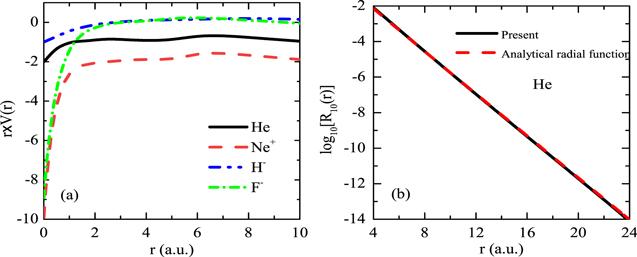
We first show the quality of potentials of atoms or ions in figure 1(a) and how to extract structure parameter C_l using the fitting procedure in figure 1(b). In figure 1(a), we can see the effective charge changes gradually from the nuclear charge to the asymptotic one. In the LBα model [30, 37, 38], we take β=0.01 and the adjustable parameter α is optimized to obtain the accurate ionization potential (IP) by comparing with the experimental IP from the NIST database [43]. The optimized α and comparison between the present calculated IPs and the experimental values are listed in table 1. In figure 1(b), it is clear that our calculated radial function decays exponentially and has a very good fitting to the asymptotic analytical form in equation (20). We systematically determined structure parameters of 25 atoms, 24 positive ions and 13 negative ions and compared with those obtained from other methods in table 2. In [8], structure parameters of five rare-gas atoms were calculated by using the self-interaction free DFT. In [44], structure parameters of Ar, Kr, and Xe were extracted from HF wave functions obtained from the X2DHF program [29]. We noticed that the structure parameter A in [24] has the same definition as the present C_l and the A parameter is found by matching the HF wave functions to the asymptotic solutions. In [7], the ionization rate depends on the coefficients ${C}_{{n}^{* }{l}^{* }}$. We mention that definitions of ${C}_{{n}^{* }{l}^{* }}$ and C_l are somewhat different and they are related by C_l=${C}_{{n}^{* }{l}^{* }}{\kappa }^{{}^{{Z}_{c}/\kappa +0.5}}$.In table 2, one can find some discrepancies among structure parameters obtained from different methods indeed. It indicates asymptotic properties of the corresponding wave functions are somewhat different. In figure 2, we take the Xe atom as an example to give a direct comparison of radial wave functions calculated by using the model potential in [13] and our numerical DFT potential, respectively. It can be seen that radial functions agree very well in small-r region. However, there are large differences for slopes of these radial functions in large-r region and thus structure parameters extracted from these radial wave functions are different (see table 2). In our DFT potential, both electrostatic potential and exchange-correlation interaction have been included. We expect structure parameters extracted using our DFT method described in section 2.2 are reliable.

Figure 1.

New window|Download| PPT slide
Figure 1.(a) The effective charge of He, Ne⁺, H⁻, and F⁻, where potentials are calculated by using the density-functional theory; (b) the structure parameter C_l of He is extracted from the electronic wave function in the asymptotic region by the fitting method.

Figure 2.

New window|Download| PPT slide
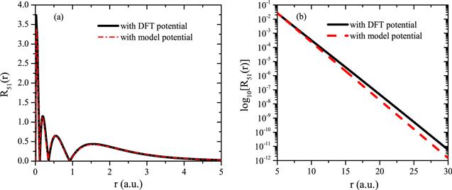
Figure 2.Radial functions of Xe in the (a) small-r region; (b) large-r region.



Table 1.
Table 1.Direct comparison of the calculated IPs using the LBα model and the experimental values from the NIST database [43]. The optimized α parameters used in LBα model are also listed.

Atom/ion	LBα (eV)	Ip (eV)	α	Atom/ion	LBα (eV)	Ip (eV)	α
H(1s)	13.60	13.60	—	He(1s)	24.59	24.59	1.34
Li(2s)	5.41	5.39	1.24	Be(2s)	9.33	9.32	1.26
B(2p)	8.27	8.30	1.20	C(2p)	11.23	11.26	1.21
N(2p)	14.47	14.53	1.22	O(2p)	13.58	13.62	1.03
F(2p)	17.38	17.42	1.11	Ne(2p)	21.65	21.56	1.20
Na(3s)	5.12	5.14	0.87	Mg(3s)	7.78	7.65	0.75
Al(3p)	5.96	5.99	1.19	Si(3p)	8.16	8.15	1.20
P(3p)	10.44	10.49	1.22	S(3p)	10.36	10.36	1.07
Cl(3p)	12.84	12.97	1.13	Ar(3p)	15.75	15.76	1.22
K(4s)	4.35	4.34	0.54	Ca(4s)	6.12	6.11	0.41
Br(4p)	11.83	11.81	0.98	Kr(4p)	13.98	14.00	0.99
Rb(5s)	4.13	4.18	0.50	I(5p)	10.55	10.45	0.85
Xe(5p)	12.16	12.13	0.95	He+(1s)	54.48	54.42	—
Li+(1s)	75.67	75.64	1.31	Be+(2s)	18.24	18.21	1.22
B+(2s)	25.18	25.16	1.21	C+(2p)	24.37	24.38	1.25
N+(2p)	29.44	29.60	1.24	O+(2p)	35.23	35.12	1.26
F+(2p)	35.03	34.97	1.21	Ne+(2p)	40.95	40.96	1.14
Na+(2p)	47.17	47.29	1.23	Mg+(3s)	15.06	15.04	0.72
Al+(3s)	18.82	18.83	0.56	Si+(3p)	16.36	16.35	1.23
P+(3p)	19.74	19.77	1.22	S+(3p)	23.35	23.34	1.25
Cl+(3p)	23.75	23.81	1.09	Ar+(3p)	27.94	27.63	1.19
K+(3p)	31.63	31.63	1.20	Ca+(4s)	11.86	11.87	0.39
Br+(4p)	21.60	21.59	1.08	Kr+(4p)	24.30	24.36	0.95
Rb+(4p)	27.35	27.29	1.15	I+(5p)	19.10	19.13	1.04
Xe+(5p)	21.15	20.98	0.92	H−(1s)	0.76	0.75	1.17
Li−(2s)	0.62	0.62	1.13	C−(2p)	1.26	1.26	1.15
O−(2p)	1.46	1.46	1.05	F−(2p)	3.40	3.40	1.14
Na−(3s)	0.54	0.55	0.72	Al−(3p)	0.44	0.44	1.11
Si−(3p)	1.39	1.39	1.17	P−(3p)	0.75	0.75	1.01
Cl−(3p)	3.61	3.62	1.17	K−(4s)	0.50	0.50	0.48
Br−(4p)	3.38	3.37	1.00	Rb−(5s)	0.49	0.49	0.43

New window|CSV


Table 2.
Table 2.The fitted C_l structure parameters versus values from earlier [7, 8, 24, 44].

Atom/ion	Cl		Atom/ion	Cl		Atom/ion	Cl
H(1s)	2.00		He(1s)	2.42		Ne(2p)	1.47
	2.00	[7]		2.98	[7]		2.77	[7]
				3.13	[8]		2.10	[8]
				2.87	[24]		1.75	[24]
				2.96a			1.95a
Ar(3p)	1.85		Kr(4p)	2.17		Xe(5p)	4.39
	2.25	[7]		2.05	[7]		1.80	[7]
	2.44	[8]		2.49	[8]		2.57	[8]
	2.11	[24]		2.22	[24]		2.40	[24]
	2.51	[44]		2.59	[44]		2.72	[44]
	2.44a			2.01a			2.55a
Li(2s)	0.56		Be(2s)	1.44		B(2p)	0.66
	0.59	[7]		1.36	[7]		1.17	[7]
	0.82	[24]		1.62	[24]		0.88	[24]
C(2p)	0.92		N(2p)	1.21		O(2p)	0.95
	1.67	[7]		2.11	[7]		2.00	[7]
	1.30	[24]		1.50	[24]		1.30	[24]
F(2p)	1.19		Na(3s)	0.32		Mg(3s)	0.79
	2.42	[7]		0.54	[7]		1.05	[7]
	1.59	[24]		0.74	[24]		1.32	[24]
Al(3p)	0.46		Si(3p)	0.98		P(3p)	1.48
	0.71	[7]		1.15	[7]		1.55	[7]
	0.61	[24]		1.10	[24]		1.65	[24]
S(3p)	1.16		Cl(3p)	1.53		K(4s)	0.26
	1.53	[7]		1.92	[7]		0.38	[7]
	1.11	[24]		1.78	[24]		0.52	[24]
Ca(4s)	0.61		Br(4p)	1.71		Rb(5s)	0.31
	0.74	[7]		1.76	[7]		0.34	[7]
	0.95	[24]		1.83	[24]		0.48	[24]
I(5p)	3.72		He+(1s)	5.66		Li+(1s)	6.03
	1.55	[7]		5.66	[7]		6.52	[7]
	1.94	[24]					6.50	[24]
Be+(2s)	2.21		B+(2s)	3.71		C+(2p)	2.17
	1.96	[7]		3.04	[7]		2.93	[7]
	2.67	[24]		6.70	[24]		2.53	[24]
N+(2p)	2.43		O+(2p)	2.88		F+(2p)	2.40
	3.62	[7]		4.23	[7]		4.21	[7]
	2.90	[24]		3.30	[24]		3.10	[24]
Ne+(2p)	2.67		Na+(2p)	2.74		Mg+(3s)	1.33
	4.76	[7]		5.23	[7]		1.41	[7]
	3.40	[24]		3.70	[24]		2.31	[24]
	3.43a
Al+(3s)	2.14		Si+(3p)	1.58		P+(3p)	2.55
	2.06	[7]		1.64	[7]		2.22	[7]
	3.10	[24]		1.80	[24]		2.50	[24]
S+(3p)	2.86		Cl+(3p)	2.96		Ar+(3p)	3.47
	2.78	[7]		2.85	[7]		3.37	[7]
	3.20	[24]		3.10	[24]		3.40	[24]
							3.81a
K+(3p)	3.59		Ca+(4s)	0.79		Br+(4p)	2.74
	3.86	[7]		0.86	[7]		2.51	[7]
	3.90	[24]		1.62	[24]		2.50	[24]
Kr+(4p)	3.55		Rb+(4p)	3.58		I+(5p)	3.60
	2.93	[7]		3.33	[7]		2.11	[7]
	3.70	[24]		3.82	[24]		2.90	[24]
Xe+(5p)	4.97		H−(1s)	0.47		Li−(2s)	0.78
	2.42	[7]		1.12a			1.00	[24]
	3.20	[24]
C−(2p)	0.45		O−(2p)	0.38		F−(2p)	0.65
	0.74	[24]		0.65	[24]		0.84	[24]
							0.76a
Na−(3s)	0.42		Al−(3p)	0.57		Si−(3p)	1.02
	1.00	[24]		0.51	[24]		1.10	[24]
P−(3p)	0.55		Cl−(3p)	1.20		K−(4s)	0.57
	0.90	[24]		1.34	[24]		0.90	[24]
Br−(4p)	1.41		Rb−(5s)	0.78
	1.49	[24]		0.80	[24]

^aThe fitted C_l coefficients using wave functions calculated by solving time-independent Schrödinger equation combined with the model potential [13, 34, 35].

New window|CSV

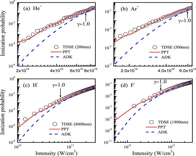
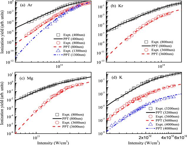
Let us turn to examine carefully the accuracy of these structure parameters in table 2. In figure 3, we compare ionization probabilities of He⁺, Ar⁺, H⁻ and F⁻ calculated using the PPT and ADK models with those obtained from the three-dimensional TDSE simulations. We mention that structure parameters extracted from our DFT wave functions are used in the PPT and ADK models. All the ionization probabilities from the PPT and ADK models are normalized to the TDSE results. One can see that all the ionization probabilities from the PPT model are in good agreement with the TDSE results in a wide intensity range covering from the multiphoton to tunneling ionization regimes, while the ADK model seriously underestimate ionization probabilities about 2–4 order of magnitude in the multiphoton region. Figure 4 compares ionization yields of Ar, Kr, Mg and K calculated from the PPT model (see equation (25)) with the experimental data [45]. In our simulations, a linearly polarized Gaussian pulse with the FWHM of 90 fs and different laser wavelengths are used. It can be seen that all the ionization yields fit perfectly the experimental results both in the multiphoton and tunneling ionization regimes.

Figure 3.

New window|Download| PPT slide
Figure 3.Comparison of ionization probabilities obtained from three different methods: (a) He⁺, (b) Ar⁺, (c) H⁻ and (d) F⁻. We take the laser field to be a Gaussian pulse with pulse duration (full width at half maximum, FWHM) of 15 fs.

Figure 4.

New window|Download| PPT slide
Figure 4.Comparison of ionization yields at several different laser wavelengths: (a) Ar, (b) Kr, (c) Mg and (d) K. The volume effect of a focused laser pulse with FWHM of 90 fs is considered. The Experimental data are from [45].

4. Conclusions

In this paper, we systematically determined structure parameters used in the ADK and PPT models for 25 atoms, 24 positive ions and 13 negative ions based on the DFT. These structure parameters are very useful for calculating ionization rate using the ADK or PPT model. Especially we present structure parameters of 24 positive ions and of 13 negative ions which should be needed to study the sequential double ionization (or detachment) probabilities based on the ADK and PPT models. We mention that structure parameters for any highly charged ions can be extracted if necessary in the future. The reliability of these structure parameters are examined carefully by comparing ionization probabilities calculated by the ADK and PPT models with those three-dimensional TDSE results. By considering the volume effect, we found that all the calculated ionization yields using the PPT model can fit perfectly the experimental data at several different laser wavelengths both in multiphoton and tunneling ionization regimes.

Acknowledgments

Project supported by the National Natural Science Foundation of China under Grant Nos. 11664035, 11864037 and 11765018. and the Foundation of Northwest Normal University (No. NWNU−LKQN−17−1).

Reference View Option By original order
By published year
By cited within times
By Impact factor

[1]Oppenheimer J R 1928 Phys. Rep. 31 66
DOI:10.1103/PhysRev.31.66 [Cited within: 1]

[2]Kulander K C 1987 Phys. Rev. A 35 445
DOI:10.1103/PhysRevA.35.445 [Cited within: 1]

[3]Tong X M Chu S I 1997 Chem. Phys. 217 119
DOI:10.1016/S0301-0104(97)00063-3 [Cited within: 2]

[4]Landau L D Lifshitz E M 2013 Quantum Mechanics: Non-Relativistic Theory vol 3 AmsterdamElsevier
[Cited within: 1]

[5]Tolstikhin O I Morishita T Madsen L B 2011 Phys. Rev. A 84 053423
DOI:10.1103/PhysRevA.84.053423 [Cited within: 1]

[6]Keldysh L V 1965 Sov. Phys. JETP 20 1307
[Cited within: 1]

[7]Ammosov M V Delone N B Krainov V P 1986 Sov. Phys - JETP 64 1191
DOI:10.1007/978-3-642-85691-4_3 [Cited within: 52]

[8]Tong X M Zhao Z X Lin C D 2002 Phys. Rev. A 66 033402
DOI:10.1103/PhysRevA.66.033402 [Cited within: 10]

[9]Zhao S F Jin C Le A T Jiang T F Lin C D 2010 Phys. Rev. A 81 033423
DOI:10.1103/PhysRevA.81.033423 [Cited within: 1]

[10]Zhao S F Xu J Jin C Le A T Lin C D 2011 J. Phys. B: At. Mol. Opt. Phys. 44 035601
DOI:10.1088/0953-4075/44/3/035601

[11]Kjeldsen T K Bisgaard C Z Madsen L B Stapelfeldt H 2005 Phys. Rev. A 71 013418
DOI:10.1103/PhysRevA.71.013418

[12]Madsen C B Madsen L B 2007 Phys. Rev. A 76 043419
DOI:10.1103/PhysRevA.76.043419 [Cited within: 1]

[13]Tong X M Lin C D 2005 J. Phys. B: At. Mol. Opt. Phys. 38 2593
DOI:10.1088/0953-4075/38/15/001 [Cited within: 7]

[14]Zhang Q Lan P Lu P 2014 Phys. Rev. A 90 043410
DOI:10.1103/PhysRevA.90.043410 [Cited within: 1]

[15]Brabec T Côté M Boulanger P Ramunno L 2005 Phys. Rev. Lett. 95 073001
DOI:10.1103/PhysRevLett.95.073001 [Cited within: 1]

[16]Hao X Zhang X Li W Chen J 2013 Phys. Rev. A 87 045403
DOI:10.1103/PhysRevA.87.045403 [Cited within: 1]

[17]Perelomov A M Popov V S Terent’ev M V 1966 Sov. Phys - JETP 23 924
[Cited within: 2]

[18]Ilkov F A Decker J E Chin S L 1992 J. Phys. B: At. Mol. Opt. Phys. 25 4005
DOI:10.1088/0953-4075/25/19/011 [Cited within: 2]

[19]Benis E P Xia J F Tong X M Faheem M Zamkov M Shan B Richard P Chang Z 2004 Phys. Rev. A 70 025401
DOI:10.1103/PhysRevA.70.025401 [Cited within: 1]

[20]Zhao S F Le A T Jin C Wang X Lin C D 2016 Phys. Rev. A 93 023413
DOI:10.1103/PhysRevA.93.023413 [Cited within: 4]

[21]Fu Y Z Zhao S F Zhou X X 2012 Chin. Phys. B 21 113101
DOI:10.1088/1674-1056/21/11/113101 [Cited within: 2]

[22]Zhao S F Lu L Zhou X X 2014 Opt. Commun. 313 74
DOI:10.1016/j.optcom.2013.09.074 [Cited within: 1]

[23]Tong X M Chu S I 1997 Phys. Rev. A 55 3406
DOI:10.1103/PhysRevA.55.3406 [Cited within: 1]

[24]Radzig A A Smirnov B M 2012 Reference Data on Atoms, Molecules, and Ions vol 31 Berlin Springer 60 85
[Cited within: 62]

[25]Frisch M J et al. 2003 GAUSSIAN 03, Revision B.04 Pittsburgh, PA Gaussian Inc.
[Cited within: 2]

[26]Schmidt M W et al. 1993 J. Comput. Chem. 14 1347
DOI:10.1002/jcc.540141112 [Cited within: 1]

[27]Madsen L B Jensen F Tolstikhin O I Morishita T 2013 Phys. Rev. A 87 013406
DOI:10.1103/PhysRevA.87.013406 [Cited within: 1]

[28]Madsen L B Jensen F Tolstikhin O I Morishita T 2014 Phys. Rev. A 89 033412
DOI:10.1103/PhysRevA.89.033412 [Cited within: 1]

[29]Kobus J Laaksonen L Sundholm D 1996 Comput. Phys. Commun. 98 346
DOI:10.1016/0010-4655(96)00098-7 [Cited within: 2]

[30]Zhao S F Jin C Le A T Lin C D 2010 Phys. Rev. A 82 035402
DOI:10.1103/PhysRevA.82.035402 [Cited within: 4]

[31]Wang J P Zhao S F Zhang C R Li W Zhou X X 2014 Mol. Phys. 112 1102
DOI:10.1080/00268976.2013.833349

[32]Zhao S F Huang F Wang G L Zhou X X 2016 Commun. Theor. Phys. 65 366
DOI:10.1088/0253-6102/65/3/366

[33]Zhao S F Li J K Wang G L Li P C Zhou X X 2017 Commun. Theor. Phys. 67 289
DOI:10.1088/0253-6102/67/3/289 [Cited within: 1]

[34]Zhou X X Chen Z Morithita T Le A T Lin C D 2008 Phys. Rev. A 77 053410
DOI:10.1103/PhysRevA.77.053410 [Cited within: 2]

[35]Laughlin C Chu S I 1993 Phys. Rev. A 48 4654
DOI:10.1103/PhysRevA.48.4654 [Cited within: 2]

[36]Zhao S F Zhou X X Li P C Chen Z 2008 Phys. Rev. A 78 063404
DOI:10.1103/PhysRevA.78.063404 [Cited within: 1]

[37]Schipper P R Gritsenko O V van Gisbergen S J Baerends E J 2000 J. Chem. Phys. 112 1344
DOI:10.1063/1.480688 [Cited within: 2]

[38]Chu S I 2005 J. Chem. Phys. 123 062207
DOI:10.1063/1.1904587 [Cited within: 2]

[39]Bachau H et al. 2001 Rep. Prog. Phys. 64 1815
DOI:10.1088/0034-4885/64/12/205 [Cited within: 1]

[40]Hu S L Zhao Z X Shi T Y 2014 Int. J. Quantum Chem. 114 441
DOI:10.1002/qua.24582

[41]Vanne Y Y Saenz A 2004 J. Phys. B: At. Mol. Opt. Phys. 37 4101
DOI:10.1088/0953-4075/37/20/005 [Cited within: 1]

[42]Augst S Meyerhofer D D Strickland D Chin S L 1991 J. Opt. Soc. Am. B 8 858
DOI:10.1364/JOSAB.8.000858 [Cited within: 1]

[43]Ralchenko Y Kramida A E Reader J (NIST ASD Team) 2008 NIST Atomic Spectra Database (version 3.1.5) Gaithersburg, MD National Institute of Standards and Technology
[Cited within: 2]

[44]Kjeldsen T K Madsen L B 2005 Phys. Rev. A 71 023411
DOI:10.1103/PhysRevA.71.023411 [Cited within: 5]

[45]Lai Y H et al. 2017 Phys. Rev. A 96 063417
DOI:10.1103/PhysRevA.96.063417 [Cited within: 2]