Li-Li Shi¹, Jian-Ping Hu¹, Yu Zhang^,1,?, Chen Ma¹, Peng-Fei Duan^2,31 Faculty of Science, Kunming University of Science and Technology, Kunming 650500, China
2 Geological Resources and Geological Engineering Postdoctoral Programme, University of Science and Technology,Kunming 650093, China
3 City College, Kunming University of Science and Technology, Kunming 650051, China

Corresponding authors: ?E-mail:zhangyu 128@126.com

Received:2019-02-25Online:2019-10-9

Fund supported:

Supported partly by the National Natural Science Foundation of China under Grant .No. 11565016 the Special Training Program for Distinguished Young Teachers of the Higher Education Institutions of Yunnan Province under Grant .No. 1096837802 the Applied Basic Research Programs of Yunnan Provincial Science and Technology Department under Grant .No. 2016FB008

Abstract
This paper aims to investigate the geodesic motion in the spacetime of a non-linear magnetic charged black hole surrounded by quintessence. By varying the Lagrangian corresponding to the metric, the orbital motion equation has been obtained. The effects of the magnetic charge $Q$, positive normalization factor $C$, angular momentum $b$, and energy $E$ on time-like and null geodesic motion are discussed from three aspects: orbital stability, orbital types, and circular orbits. By comparing the effects of the above parameters $C$, $b$ on the effective potential, it is found that quintessence has an impact on the types and stability of orbits. In addition, for time-like orbital motion, when $3.443113\leq b\leq6.392\,578$ (for fixed $C=0.0002$, $M = 1$, $Q=0.7$), there are bound orbits, and within this range, the stable circular orbits exist, and the radii of the innermost and outermost stable circular orbit are $r=5.912\,654$ and $r=56.745\,933$, respectively. For null orbital motion, the orbital types have only unstable circular orbit which occur at $r=2.951\,072$ ($E^{2}=E_{2}^{2}=0.4$), absorb orbits and escape orbits, but no stable circular orbits, and bound orbits.
Keywords： effective potential;orbital stability;orbital types


PDF (1126KB)MetadataMetricsRelated articlesExportEndNote|Ris|BibtexFavorite
Cite this article
Li-Li Shi, Jian-Ping Hu, Yu Zhang, Chen Ma, Peng-Fei Duan. Geodesic Structure of a Non-linear Magnetic Charged Black Hole Surrounded by Quintessence. [J], 2019, 71(10): 1187-1195 doi:10.1088/0253-6102/71/10/1187

1 Introduction

Cosmological observations such as the cosmic microwave background, baryon acoustic oscillation, Hubble measurements, and the supernovae type Ia^[1-2] suggest that our universe is undergoing an accelerated phase of expansion. Astrophysicists and cosmologists believe that the reason for the accelerated expansion of the universe is due to dark energy.^[3-4] According to observations, more than seventy percent of the universe are composed of dark energy.

Quintessence is one of the candidates for dark energy, with negative state parameter $w_{q}$ (the ratio of pressure to density), and $-1<w_{q}<-{1}/{3}$. In 2003, Kiselev^[5] derived a spherical symmetric solution of the Einstein equations describing the Schwarzschild black hole surrounded by quintessence, which attracted wide attention of researchers. Using WKB approximation approach, quasinormal modes of a black hole surrounded by quintessence have been studied in Refs. ^[6-14] . The existence of Nariai type black holes with quintessence for special values of the parameters in the theory has been shown by Fernando.^[15] And he also investigated the properties of the charged black hole surrounded by the quintessence.^[16] The solution of non-linear magnetic charged black hole surrounded by quintessence is derived in Ref. ^[17] . The quintessence around the black hole also corrects the thermodynamic quantities. By using the improved brick-wall model, Ma et al.^[18] evaluated the entropy of a Schwarzschild spacetime surrounded with the quintessence. In Ref. ^[19] , a solution of Einstein equations with quintessential matter surrounding a d-dimensional black hole is found, then the Hawking radiation in this black hole background has been investigated. Azreg-Anou^[20] has obtained the quintessence-dependent enthalpy and new extreme solutions in charged de Sitter-like black holes. The thermodynamic stabilities of uncharged and charged black holes surrounded by quintessence have been studied in Ref. ^[21] .

Furthermore, the study of the geodesic structure helps us to understand different gravitational properties of a gravitational center, especially in the strong field regime, like neutron stars and black hole. In recent years, the field on the geodesic motion in the black hole became a fertile ground for researchers^[22-37] from different point of view. In Schwarzschild AdS black hole spacetime, a complete discussion for the geodesic motion has been made in Ref. ^[38] , they found all kinds of orbits, which are permitted according to the energy levels. Enolskii et al.^[39] studied the particle motion in Kehagias-Sfetsos black hole spacetime, which is a static spherically symmetric solution of a Horava-Lifshitz gravity model. Malakolkalami and Ghaderi^[40] analyzed the null geodesics and all types of orbital motion in the Schwarzschild-anti de Sitter black hole surrounded by quintessence spacetime by means of the effective potential for the photons.

In this paper we discuss geodesic motion in the spacetime of the non-linear magnetic charged black hole surrounded by quintessence. The organization of this work is as follows. In the second sections, we obtain the equations of geodesic motion by varying the Lagrangian. In the third and fourth sections, we mainly concentrate on the influence of magnetic charge $Q$, energy levels $E$, positive normalization factor $C$, angular momentum $b$ on the geodesic motion of time-like and null. In the last section, the conclusion is drawn.

2 Equations of the Orbital Motion

The metric of the spacetime of non-linear magnetic charged black hole surrounded by quintessence is given by^[17]

(1)$$ d s^{2}=-g(r)d t^{2}+\frac{1}{g(r)}d r^{2}+r^{2}d\theta^{2}+r^{2}\sin^{2}\theta d\phi^{2}\,, $$
with

(2)$$ g(r)=1-\frac{2Mr^{2}}{r^{3}+Q^{3}}-\frac{C}{r^{3w_{q}+1}}\,,$$
where $M$ denotes the black hole mass, $C$ respects the positive normalization factor, $Q$ is the magnetic charge. $w_{q}$ is the quintessential state parameter, which is constrained to the interval $-1<w_{q}<-{1}/{3}$. It is obvious that when $C=0$ the metric is the Hayward-like black hole metric; when $Q=0$ the metric is the Schwarzschild solution surrounded by quintessence; when $Q=0$, $C=0$ it is the Schwarzschild black hole one.

Then, from here on we put particle mass $m=1$, this means that the related parameters are expressed in units of $m$. The Lagrangian corresponding to the metric Eq. (1) is

(3)$$ L=\frac{1}{2}(-g(r)\dot{t}^{2}+g(r)^{-1}\dot{r}^{2}+r^{2}\dot{\phi}^{2})\,,$$
where a dot represents differentiation with respect to the affine parameter, $\tau$. The Euler-Lagrange equation is

(4)$$ \frac{d}{d\tau}\Big(\frac{\partial L}{\partial \dot{x}^{\nu}}\Big)-\frac{\partial L}{\partial x^{\nu}}=0\,. $$
By substituting Eq. (4) into Eq. (3), we can get

(5)$$ \dot{t}=\frac{E}{g(r)}\,, \quad r^{2}\sin^{2}\theta\dot{\phi}=b\,.$$
Without loss of generality, we put $\theta={\pi}/{2}$. Then Eq. (5) can be written as

(6)$$ \dot{t}=\frac{E}{g(r)}\,, \quad \dot{\phi}=\frac{b}{r^{2}}\,.$$
Substituting Eq. (6) into Eq. (3), we can get

(7)$$ \dot{r}^{2}=E^{2}-\Big(1-\frac{2Mr^{2}}{r^{3}+Q^{3}}-\frac{C}{r^{3w_{q}+1}}\Big) \Big(\frac{b^{2}}{r^{2}}+L\Big)\,. $$
Here, the effective potential equation can be defined as

(8) $$ V_{eff}^{2}=\Big(1-\frac{2Mr^{2}}{r^{3}+Q^{3}}-\frac{C}{r^{3w_{q}+1}}\Big)\Big(\frac{b^{2}}{r^{2}}+L\Big)\,.$$
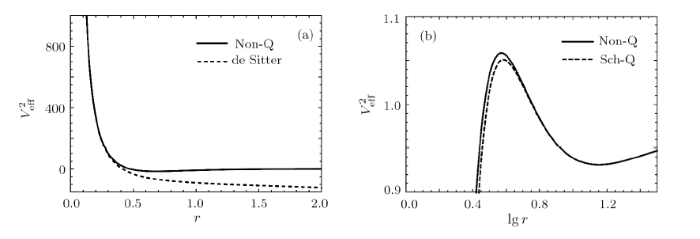
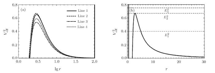
Now we have obtained the effective potential equation in the non-linear magnetic charged black hole surrounded by quintessence spacetime. Interestingly, in the case of short distances ($Q/r\gg1$), the function $g(r)\simeq1-{\Lambda r^{2}}/{3}-{C}/{r^{3w_{q}+1}}$, with $\Lambda=6M/Q^{3}$, the effective potential equation is $V_{eff}^{2}=g(r)({b^{2}}/{r^{2}}+1)$. Comparing the two curves in Fig. 1(a), we can see that the behavior curves of non-linear magnetic charged black hole surrounded by quintessence spacetime and de-Sitter geometry are very similar as $Q/r\gg1$. However, there is no circular orbit in de-Sitter geometry. In the case of large distances ($Q/r\ll1$), the function $g(r)=1-{2M}/{r}-{C}/{r^{3w_{q}+1}}$, the effective potential equation is $V_{eff}^{2}=g(r)({b^{2}}/{r^{2}}+1)$. It is shown in Fig. 1(b) that the behavior of the effective potential of particle in non-linear magnetic charged black hole surrounded by quintessence is similar to a Schwarzschild black hole surrounded by quintessence, especially $Q/r\ll1$.

New window|Download| PPT slide
Fig.1(a) The behaviors of the effective potential of particle in non-linear magnetic charged black hole surrounded by quintessence (Non-Q) and de-Sitter geometry for fixed $b = 4.2$, $M = 1$, $Q=0.7$, $C=0.0002$. (b) The behaviors of the effective potential of particle in non-linear magnetic charged black hole surrounded by quintessence (Non-Q) and Schwarzschild black hole surrounded by quintessence (Sch-Q) for fixed $b = 4.2$, $M = 1$, $Q=0.7$, $C=0.0002$.

New window|Download| PPT slide
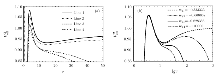
Fig.2(a) The behaviors of the effective potential of particle with different $w_{q}$ for fixed other different parameters. Line 1 represents $w_{q}=-0.4$, $C=0.001$, $b = 4.3$, $M = 1$, $Q=0.5$; Line 2 represents $w_{q}=-0.6$, $C=0.0008$, $b = 4.2$, $M = 1$, $Q=0.7$; Line 3 represents $w_{q}=-0.8$, $C=0.0008$, $b = 4.1$, $M = 1$, $Q=0.5$; Line 4 represents $w_{q}=-0.8$, $C=0.0006$, $b = 4.0$, $M = 1$, $Q=0.3$. (b) The behaviors of the effective potential of particle with different $w_{q}$ for fixed $b = 4.2$, $M = 1$, $C=0.0002$, $Q=0.7$.



Furthermore, Fig. 2(a) shows the behaviors of the effective potential of particle with different $w_{q}$ for fixed different values of other parameters $Q$, $C$, $b$. In order to better analyze the orbital types of particle or photon with various parameters, we consider the parameter range that can make the orbital types at most (the existence of stable circular orbits and bound orbits). Taking $b = 4.2$, $M = 1$, $C=0.0002$, $Q=0.7$ as an example, Fig. 2(b) clearly shows that when $-0.838\,356\leq w_{q}<-{1}/{3}$, the orbital types are the most, including absorb orbits, unstable circular orbits, stable circular orbits, bound orbits, and escape orbits; when $-1<w_{q}<-0.838\,356$, there are only absorb orbits, unstable circular orbits, and escape orbits, but no bound orbits and stable circular orbits for the orbital types. Obviously, the effective potential analysis of the former is more representative than that of the latter, and the orbital types of the former includes all the orbital types of the latter. For convenience, this paper we consider the case of state parameter $w_{q}=-{2}/{3}$ (when $w_{q}$ takes other values, the analysis is similar) and the parameter range that can make the orbital types at most (the existence of stable circular orbits and bound orbits).

3 Time-Like Orbital Motion

In the case of time-like geodesics, we have that $L=1$, Eq. (8) can be rewritten as follows:

(9)$$ V_{eff}^{2}=\Big(1-\frac{2Mr^{2}}{r^{3}+Q^{3}}-\frac{C}{r^{3w_{q}+1}}\Big)\Big(\frac{b^{2}}{r^{2}}+1\Big)\,. $$
In this section, we aim to obtain the influence of positive normalization factor $C$, magnetic charge $Q$, angular momentum $b$, and energy $E$ on the geodesic motion for fixed black hole mass $M=1$.

3.1 Magnetic Charge $Q$

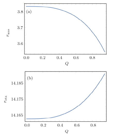
In Fig. 3, the dependence of the effective potential is shown with different values of $Q$ for fixed $b = 4.2$, $M=1$, $C=0.0002$. From this figure one can easily see that with the decrease of magnetic charge $Q$, the peak of curves is going to be decreased, the location of peak and the intersection of the effective potential and $r$-axis come far away the central of black hole. Moreover, one can conclude from Fig. 4 that as $Q$ increases, the radius of the unstable circular orbit decreases, while the radius of the stable circular orbit increases. In this case, the radius of the unstable and stable circular orbit in Schwarzschild and Schwarzschild solution surrounded by quintessence (Sch-Q) are 3.832 776, 13.807 224; 3.833 210, 14.162 434, respectively. Comparing the radius of circular orbit under three spacetime conditions, we can see that for the radius of unstable circular orbit: $r_{\text{Sch-Q}}>r_{\rm Sch}>r_{\rm Non}$, for the radius of stable circular $r_{\rm Sch}<r_{\text{Sch-Q}}<r_{\text{Non-Q}}$.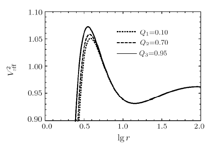

New window|Download| PPT slide
Fig.3The behaviors of the effective potential of particle with different $Q$ for fixed $b = 4.2$, $M = 1$, $C=0.0002$.

3.2 Positive Normalization Factor $C$

In the case of $C=0$, there is no quintessence, the equations of the orbital motion, and the corresponding effective potential are as follows:

(10)$$ \dot{r}^{2}=E^{2}-V_{eff}^{2}\,$$
(11)$$ V_{eff}^{2}=\Big(1-\frac{2Mr^{2}}{r^{3}+Q^{3}}\Big)\Big(\frac{b^{2}}{r^{2}}+1\Big)\,.$$
In the case of $C\neq0$, there is quintessence, then the equations of the orbital motion and corresponding effective potential are as follows:

(12)$$ \dot{r}^{2}=E^{2}-V_{eff}^{2}\,$$
(13)$$ V_{eff}^{2}=\Big(1-\frac{2Mr^{2}}{r^{3}+Q^{3}}-rC\Big)\Big(\frac{b^{2}}{r^{2}}+1\Big)\,.$$
For the circular orbits, the corresponding effective potential must satisfy

(14)$$ E^{2}=V_{eff}^{2}\,,$$
(15)$$ \frac{d V_{eff}^{2}}{d r}=0\,.$$
In order to obtain a critical value that can be used to determine the occurrence of a stable circular orbit, we still need guarantee follows equation simultaneously

(16)$$ \frac{d^{2}V_{eff}^{2}}{d r^{2}}=0\,.$$

New window|Download| PPT slide
Fig.4The radius of the unstable circular orbit $r_{\rm uns}$ (a) and the radius of the stable circular orbit $r_{\rm sta}$ (b) of particle with different $Q$ for fixed $C = 0.0002$, $M = 1$, $b=4.2$.



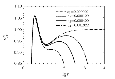
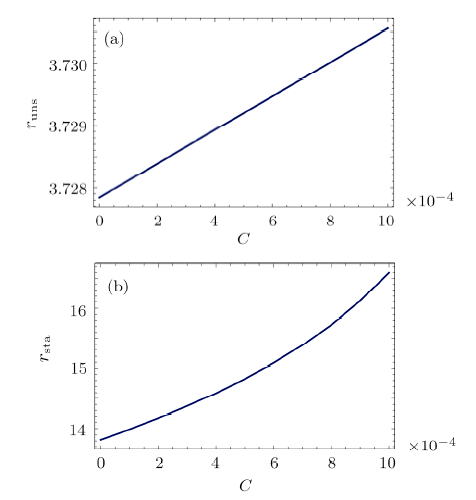
By solving the above Eq. (13) to Eq. (16), we get the critical value $C=0.001\,322$, which represents the radius of the outermost circular orbit is $r=21.236\,694\,3$. In Fig. 5, the effective potential of the particle motion with different $C$ is shown, where we fix parameters $b = 4.2$, $M = 1$, $Q=0.7$. When $C\leq0.001\,322$, for example $C=0.0001$ and $C=0.0004$, the stable circular orbit exists; when $C>0.001\,322$, the stable circular orbit disappears. Furthermore, the peak of effective potential curve increases with the decrease of $C$. With respect to the radius of the unstable circular orbits ($r_{\rm uns}$) and stable circular orbits ($r_{\rm sta}$) on $C$, $r_{\rm uns}$ and $r_{\rm sta}$ increase as $C$ increases, as shown in Fig. 6. Similarly, when the parameters $Q$ and $b$ are $Q_{1}=0.7$, $b_{1}=3.8$; $Q_{2}=0.5$, $b_{2}=3.8$; $Q_{3}=0.3$, $b_{3}=4.2$; the corresponding parameters $C$ which can make the stable circular orbits exist are $C_{1}\leq0.002\,205$, $C_{2}\leq0.002\,207$, $C_{3}\leq0.001\,323$.

New window|Download| PPT slide
Fig.5The behaviors of the effective potential of particle with different $C$ for fixed $b = 4.2$, $M = 1$, $Q=0.7$.

New window|Download| PPT slide
Fig.6The radius of the unstable circular orbit $r_{\rm uns}$ (a) and the radius of the stable circular orbit $r_{\rm sta}$ (b) of particle with different $C$ for fixed $Q = 0.7$, $M = 1$, $b=4.2$.

3.3 Angular momentum b

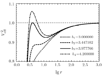
Generally speaking, it is clear that there is a critical value of $b$ for which the geodesic equations allow a stable circular orbit. In Fig. 7, the effective potential of the particle motion with different values of angular momentum $b$ is shown, where we fix parameters $M=1$, $Q=0.7$, $C=0$. On the one hand, We can find that

(i) In the case of $b>3.447\,102$ (such as $b=4.2$), there are two extreme points corresponding to two circular orbits. One of them is unstable circular orbit and the other is stable circular orbit.

(ii) In the case of $b=3.447\,102$, the local maximum and minimum of the effective potential curve merge into one inflection, which corresponds to the innermost stable circular orbit occurring at $r=5.891\,429$.

(iii) In the case of $b<3.447\,102$ (such as $b=3.0$), the local minimum point of curve disappear, that is, no stable circular orbits exist. Because the angular momentum is too small for a test particle to make circular orbital motion at this time.

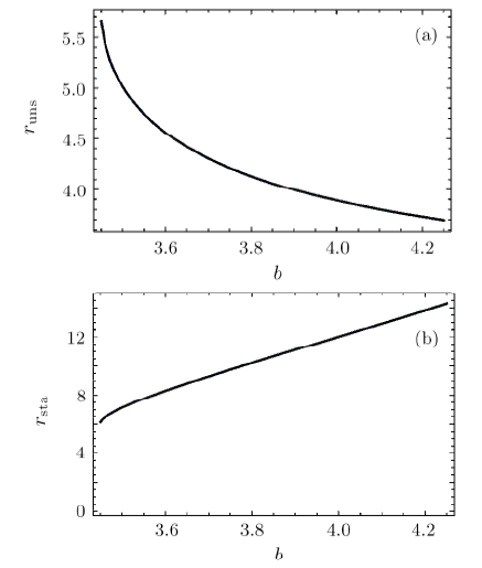
(iv) Furthermore, as $b$ increases, the radius of the unstable circular orbits decrease, while the radius of the stable circular orbits increase, as seen more explicitly in Fig. 8.

New window|Download| PPT slide
Fig. 7The behaviors of the effective potential of particle with different $b$ for fixed $C=0$, $M = 1$, $Q=0.7$.

New window|Download| PPT slide
Fig. 8The radius of the unstable circular orbit $r_{\rm uns}$ (a) and the radius of the stable circular orbit $r_{\rm sta}$ (b) of particle with different $b$ for fixed $Q = 0.7$, $M = 1$, $C=0$.



On the other hand, the results obtained indicate that

(v) If $b\leq3.977\,766$, the maximum values of the curve are less than or equal to 1. When a test particle in an unstable circular orbits is subject to any disturbance, it either falls into the black hole or enters into bound orbits. In other word, the orbital types of test particle have absorb orbits, bound orbits and circular orbits, including stable circular orbits and unstable circular orbits.

(vi) If $b>3.977\,766$, the maximum value of the curve is greater than 1, which shows that when the test particle moves on an unstable circular orbit, once it is subject to any disturbance, it may fall into the black hole or escape to infinity. This indicates that the orbital types of test particle have absorb orbits, bound orbits, circular orbits, and escape orbits.

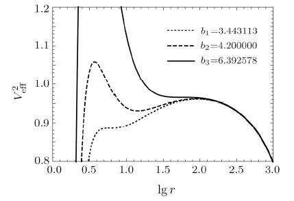
In Fig. 9 the effective potential of the particle motion with different values of angular momentum $b$ is shown, where we fix parameters $M=1$, $Q=0.7$, $C=0.0002$. We can find that

New window|Download| PPT slide
Fig. 9The behaviors of the effective potential of particle with different $b$ for fixed $C=0.0002$, $M = 1$, $Q=0.7$.



(i) When $b=3.443\, 113$, the curve has an inflection point, which corresponds to the innermost stable circular orbit with the radius $r_{\text{Non-Q}}=5.912 \,654$. Similarly, the innermost stable circular orbit radius of the Schwarzschild black hole is $r_{\rm Sch}=6$ when $b=2\sqrt{3}$. It is clearly indicate that the innermost stable circular orbit: $r_{\text{Non-Q}}<r_{\rm Sch}$.

When $b=6.392\,578$, the curve also has an inflection point, which corresponds to the outermost stable circular orbit with the radius $r=$ 56.745 933. In both cases, orbital types of motion do not include bound orbits, and only include circular orbits, escape orbits and absorb orbits.

(ii) When $3.443\,113<b<6.392\,578$, there are two extreme points corresponding to two circular orbits. One of them is unstable circular orbit and the other is stable circular orbit. Under this condition, the corresponding types of orbits include circular orbits, escape orbits, bound orbits and absorb orbits.

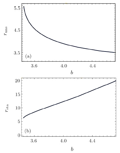
(iii) As $b$ increases, the location of the potential barrier maximum value moves to the $r$-axis left, while its location of minimum value moves to the $r$-axis right, that is, the radius of the unstable circular orbit decreases, while the radius of the stable circular orbit increases, as shown in Fig. 10.

New window|Download| PPT slide
Fig. 10The radius of the unstable circular orbit $r_{\rm uns}$ (a) and the radius of the stable circular orbit $r_{\rm sta}$ (b) of particle with different $b$ for fixed $Q = 0.7$, $M = 1$, $C=0.0002$.



From the above discussion, we can see that quintessence has an impact on the types and stability of orbits. If there is no quintessence: when $r\rightarrow\infty$, then $V_{eff}^{2}$ tends to $1$.

At $b>3.977 \,766$, there are escape orbits. When $b\geq3.447\, 102$, there are bound orbits, and in this interval, stable circular orbits appear, and the innermost stable circular orbit occurring at $r=5.891\, 429$.

If there is quintessence: when $r\rightarrow\infty$, then $V_{eff}^{2}$ tends to infinity. Regardless of the value of $b$, the escape orbits exist. When $3.443\,113\leq b\leq6.392\,578$, there are bound orbits, and within this range, there are stable circular orbits, and the radii of the innermost and outermost stable circular orbit are $r=5.912\,654$ and $r=56.745\,933$, respectively. Similarly, when the parameters $Q$ and $C$ are $Q_{1}=0.5$, $C_{1}=0.001$; $Q_{2}=0.5$, $C_{2}=0.0005$; $Q_{3}=0.7$, $C_{3}=0.0005$; the corresponding parameters $C$ which can make the stable circular orbits exist are $3.436810\leq b_{1}\leq4.451\,531$, $3.447\,618\leq b_{2}\leq5.178\,742$, $3.437\,019\leq b_{3}\leq5.178\,666$.

3.4 Energy Levels $E$

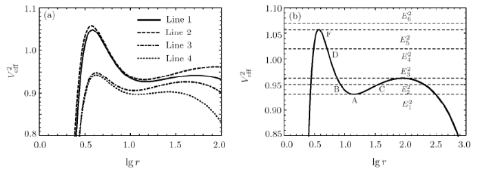
We assume the test particle initial state is to fly towards the black hole. In Fig. 11, from the analyze of the previous subsections, it is shown that when the parameters take the appropriate values, the orbital types will include stable circular orbits and bound orbits. From Fig. 11(a), it can be concluded that although the values of each parameter are different, their effective potential behavior curves are very similar. That is to say, their orbital analyze is similar. Therefore, without loss of generality, we take parameter $M=1$, $Q=0.7$, $b=4.2$, $C=0.0002$ as an example (as seen in Fig. 11(b)) to make a detailed analyze. We can draw some conclusions as follows:

(i) In the case of $E^{2}>E_{5}^{2}$ (such as $E^{2}=E_{6}^{2}=1.07$), the test particle will be swallowed by black hole starting from a finite distance.

(ii) In the case of $E^{2}=E_{5}^{2}=1.058\,155$, the test particle may orbit on unstable circular orbit at $r_{F}=3.728\,386$, when the particle is disturbed, it may fall into black holes or escape to infinity.

(iii) In the case of $E_{3}^{2}<E^{2}<E_{5}^{2}$ (such as $E^{2}=E_{4}^{2}=1.02$), the test particle may have a escape orbit, it moves to point D from infinity, then they will deflect and fly toward infinity.

New window|Download| PPT slide
Fig. 11(a) The behaviors of the effective potential of particle with different energy levels for fixed different parameters. Line 1 represents $C=0.0005$, $b = 4.2$, $M = 1$, $Q=0.3$; Line 2 represents $C=0.0002$, $b = 4.2$, $M = 1$, $Q=0.7$; Line 3 represents $C=0.0008$, $b = 3.8$, $M = 1$, $Q=0.5$; Line 4 represents $C=0.0015$, $b = 3.8$, $M = 1$, $Q=0.5$. (b) The behaviors of the effective potential of the test particle with different energy levels when we fix $M=1$, $Q=0.7$, $b=4.2$, $C=0.0002$.



(iv) In the case of $E_{1}^{2}<E^{2}<E_{3}^{2}$ (such as $E^{2}=E_{2}^{2}=0.95$), the test particle presents a bounded orbital motion between $r_{B}=8.445\,032$ (aphelion distances) and $r_{C}=35.997\,248$ (perihelion distances), respectively. On the left side of the barrier, the particle may fall into the black hole. On the right side of the barrier, the particle may escape to infinity.

(v) In the case of $E^{2}=E_{1}^{2}=0.931\,246$, the test particle will move on a stable circular orbit with radius $r_{A}=14.173\,833$.

(vi) In the case of $E^{2}<E_{1}^{2}$, the test particle may be wallowed by black hole or escape to infinity.

4 Null Orbital Motion

In the case of null geodesics, we have that $L=0$, Eq. (8) can be rewritten as follows:

(17)$$ V_{eff}^{2}=\Big(1-\frac{2Mr^{2}}{r^{3}+Q^{3}}-\frac{C}{r^{3w_{q}+1}}\Big) \Big(\frac{b^{2}}{r^{2}}\Big)\,.$$

4.1 Magnetic Charge $Q$

From Eq. (17), one can plot the behaviors of the effective potential of photon with different $Q$ values for fixed $b=4.2$, $M=1$, $C=0.0002$ as shown in Fig. 12. It is easy to find that for any values of $Q$, the effective potential only has one maximum value. As $Q$ increases, the effective potential barrier decreases and its position moves in the direction of increasing $r$, which means that the radius of the unstable circular orbit increases, as seen more explicitly in Fig. 13. At this time, the value of the intersection of the effective potential curve and the $r$-axis also increases, that is, the corresponding horizon radius is increasing. In this case, the radius of the unstable circular orbit in Schwarzschild and Schwarzschild solution surrounded by quintessence (Sch-Q) are 3.000 000, 3.000 901, respectively. Comparing the radius of circular orbit under three spacetime conditions, we can see that for the radius of unstable circular orbit: $r_{\text{Sch-Q}} > r_{\rm Sch} > r_{\text{Non-Q}}$.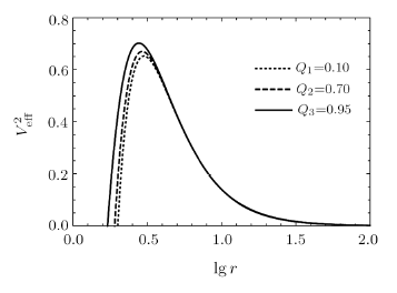

New window|Download| PPT slide
Fig. 12The behaviors of the effective potential of photon with different $Q$ values for fixed $b = 4.2$, $M = 1$, $C=0.0002$.

New window|Download| PPT slide
Fig. 13The radius of the unstable circular orbits of photon $r_{\rm uns}$ with different $Q$ values for fixed $b = 4.2$, $M = 1$, $C=0.0002$.

4.2 Positive Normalization Factor $C$

From Fig. 14 we can know that no matter how much $C$ is taken, the effective potential barrier has only one maximum value. In other words, only the unstable circular orbits exist. The peak value of effective potential barrier gets higher with $b$ increasing. Moreover, one can conclude from Fig. 15 that as $C$ increases, the radius of the unstable circular orbit increases.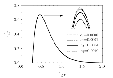

New window|Download| PPT slide
Fig. 14The behaviors of the effective potential of photon with different $C$ for fixed $b = 4.2$, $M = 1$, $Q=0.7$.

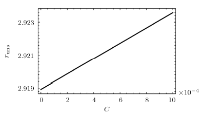New window|Download| PPT slide
Fig. 15The radius of the unstable circular orbits of photon $r_{\rm uns}$ with different $C$ values for fixed $b = 4.2$, $M = 1$, $Q=0.7$.

4.3 Angular Momentum b

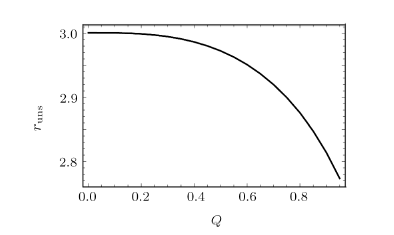
It can be clearly seen from Fig. 16 that the change of $b$ is only related to the maximum value of the effective potential. When $b$ is larger and larger, the maximum value of the effective potential also becomes larger, but the corresponding $r=2.918\,581$ remains unchanged, that is, the change of $b$ does not affect the radius of the unstable circular orbits.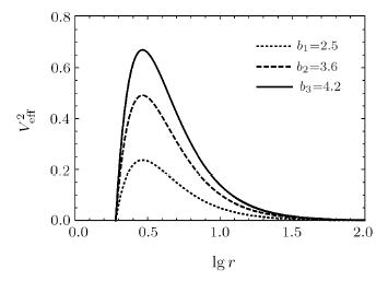

New window|Download| PPT slide
Fig. 16The behaviors of the effective potential of photon with different $b$ values for fixed $C = 0.0002$, $M = 1$, $Q=0.7$.

4.4 Energy Levels $E$

Based on the previous analyze of the parameters and Fig. 17(a), it is obvious that the shape of the effective potential behavior curve will not change significantly regardless of the values of these parameters. Therefore, without loss of generality, we take the appropriate range ($C=0.0002$, $b = 4.2$, $M = 1$, $Q=0.7$) as an example (Fig. 17(b) to analyze the influence of different energy levels on photon motion.

In Fig. 17, we assume the test photon initial state is to fly towards the black hole. Then we can obtain the following conclusions:

(i) When $E^{2}=E_{1}^{2}=0.4$, the test photon with sufficient energy on the left side of the effective potential barrier may fall into the black hole, while the test photon on the right side of the effective potential barrier will escape to infinity.

(ii) When $E^{2}=E_{2}^{2}=0.669\,884$, the test photon with sufficient energy may orbit on an unstable circular orbit with radius $r=2.951\,072$. When a photon is disturbed, the photon may fall into the black hole or escape to infinity.

(iii) When $E^{2}=E_{3}^{2}=0.7$, the test photon may fall into the black hole.

New window|Download| PPT slide
Fig. 17(a) The behaviors of the effective potential of photon with different energy levels for fixed different parameters. Line 1 represents $C=0.0005$, $b = 4.2$, $M = 1$, $Q=0.3$; Line 2 represents $C=0.0002$, $b = 4.2$, $M = 1$, $Q=0.7$; Line 3 represents $C=0.0008$, $b = 3.8$, $M = 1$, $Q=0.5$; Line 4 represents $C=0.0015$, $b = 4.0$, $M = 1$, $Q=0.5$. (b) The behaviors of the effective potential of photon with different energy levels for fixed $C=0.0002$, $b = 4.2$, $M = 1$, $Q=0.7$.

5 Conclusions

We have discussed geodesic motion in the spacetime of the non-linear magnetic charged black hole surrounded by quintessence. By varying the Lagrangian corresponding to the metric, the orbital motion equation has been obtained. It is concluded that the behavior curves of non-linear magnetic charged black hole surrounded by quintessence spacetime and de-Sitter geometry are very similar as $Q/r\gg1$, but when $Q/r\ll1$, the behavior of the effective potential of particle in non-linear magnetic charged black hole surrounded by quintessence is similar to a Schwarzschild black hole surrounded by quintessence. Then, the effects of the magnetic charge $Q$, positive normalization factor $C$, angular momentum $b$ and energy $E$ on the effective potential behavior are discussed detailed from the view of time-like and null. From the effective potential behavior curves of different parameters with different values, we can see that when we consider the existence of stable circular orbits and bound orbits, although different parameters take different values, the shape of the effective potential behavior curve is similar, that is, the analysis of the effective potential behavior is similar, so we take a set of specific values as an example to illustrate.

From the perspective of magnetic charge $Q$, whether it is time-like or null orbital motion, the parameter $Q$ has a similar effect on unstable circular radius, that is, as $Q$ increases, the unstable circular radius increases. At the same time, the value of the intersection of the curve and the $r$-axis is decreasing. But for the time-like orbital motion, as $Q$ increases, the stable circular radius decreases.

For time-like orbital motion, we fixed $M = 1$, $Q=0.7$. If there is no quintessence ($C=0$): the escape orbits only appear at $b>3.977\;766$ and the bound orbits only occur at $b\geq3.447\,012$. The radius of the innermost stable circular orbit $r=5.891\,429$. If there is quintessence ($C\neq0$): the escape orbits always exist regardless of $b$ values. The interval in which the bound orbits exist is $3.443\,113\leq b\leq6.392\,578$. The radius of the innermost stable circular orbit and outermost stable circular orbit are $r=5.912\,654$, $r=56.745\,933$, respectively. It is obvious that quintessence not only affects the types and stability of orbits, but also leads to an increase in the radius of the innermost stable circular orbit. Compared with the innermost stable circular orbit radius of the Schwarzschild black hole, it clearly indicates that $r_{\text{Non-Q}}<r_{\rm Sch}$. For null orbital motion, whatever $C$ and $b$ are, only unstable circular orbits exist.

As for the different energy levels to the types of orbit for $b=4.2$, $C=0.0002$, $M = 1$, $Q=0.7$. We assume the test particle initial state is to fly towards the black hole. For time-like orbital motion, due to the different energy levels, the orbital types include absorb orbits, bound orbits, escape orbits, and circular orbits. Unstable circular orbit occur at $r_{F}=3.768\,282$ ($E^{2}=E_{4}^{2}=1.055\,286$), stable circular orbit occur at $r_{A}=14.169\,618$ ($E^{2}=E_{1}^{2}=0.931\,239$), and the bounded orbital motion shows between aphelion distances ($r_{B}=8.438\,773$) and perihelion distances ($r_{C}=35.997\,482$), respectively (at this time $E^{2}=E_{2}^{2}=0.95$). For null orbital motion, there are only unstable circular orbit which occur at $r=2.951\,072$ ($E^{2}=E_{2}^{2}=0.4$), absorb orbits and escape orbits, but no stable circular orbits and bound orbits.

Reference View Option By original order
By published year
By cited within times
By Impact factor

[1] A. G. Riess, A. V. Filippenko, P. Challis , Astron. J. 116(1998) 1009.
[Cited within: 1]

[2] S. Perlmutter, G. Aldering, G. Goldhaber , Astron. J. 517(1999) 565.
[Cited within: 1]

[3] D. Huterer and M. S. Turner , Phys. Rev. D 60(1999) 081301.
[Cited within: 1]

[4] S. Perlmutter, M. S. Turner, M. White , Phys. Rev. Lett. 83(1999) 670.
[Cited within: 1]

[5] V. V. Kiselev , Class. Quantum Grav. 20(2003) 1187.
[Cited within: 1]

[6] S.B Chen .and J. L. Jing, Class. Quantum Grav. 22(2005) 4651.
[Cited within: 1]

[7] Y. Zhang and Y.X. Gui, , Class. Quantum Grav. 23(2006) 6141.


[8] Y. Zhang, Y. X. Gui, F. Yu, F. L. Li , Gen. Relativ. Gravit. 39(2007) 1003.


[9] C. R. Ma, Y. X. Gui, W. Wang, F. J. Wang , Centr. Eur. J. Phys. 6(2008) 194.


[10] N. Varghese and V.C. Kuriakose, , Gen. Relativ. Gravit. 41(2009) 1249.


[11] Y. Zhang, C. Y. Wang, Y. X. Gui , Chin. Phys. Lett. 26(2009) 030401.


[12] M. Saleh, B. B. Thomas, T. C. Kofane , Chin. Phys. Lett. 26(2009) 109802.


[13] M. Saleh, B. B. Thomas, T. C. Kofane , Eur. Phys. J. C 78(2018) 325


[14] J. Liang , Commun. Theor. Phys. 70(2018) 695.
[Cited within: 1]

[15] S. Fernando , Mod. Phys. Lett. A 28(2013) 1350189.
[Cited within: 1]

[16] S. Fernando , Gen. Relat. Gravit. 45(2013) 2053.
[Cited within: 1]

[17] C. H. Nam , Gen. Relativ. Gravit. 50(2018) 57.
[Cited within: 2]

[18] C. R. Ma, Y. X. Gui, F. J. Wang , Chin. Phys. Lett. 24(2007) 3286.
[Cited within: 1]

[19] S. B. Chen, B. Wang, R. K. Su , Phys. Rev. D 77(2008) 124011.
[Cited within: 1]

[20] M. Azreg-Anou , Eur. Phys. J. C 75(2015) 34.
[Cited within: 1]

[21] M. S. Ma, R. Zhao, Y. Q. Ma , Gen. Relativ. Gravit. 49(2017) 79.
[Cited within: 1]

[22] J. Podolsky , Gen. Relativ. Gravit. 31(1999) 1703.
[Cited within: 1]

[23] S. Fernando, D. Krug, C. Curry , Gen. Relat. Gravit. 35(2003) 1243.


[24] C. Leiva, J. Saavedra, J. Villanueva , Mod. Phys. Lett. A 24(2009) 1443.


[25] S. Fernando , Phys. Rev. D 85(2012) 024033.


[26] U . Kosti?, Gen. Relativ., Gravit. 44(2012) 1057.


[27] S. Grunau and V. Kagramanova , Phys. Rev. D 83(2011) 044009.


[28] A. Larranaga , Rom. J. Phys. 58(2013) 50.


[29] D.X. Kong . and X. Y .Li, Commun. Theor. Phys. 59(2013) 80.


[30] G. Abbas and U. Sabiullah , Astrophys. Space Sci. 352(2014) 769.


[31] S. Fernando, S. Meadows, K. Reis , Int. J. Theor. Phys. 54(2015) 3634.


[32] I. Hussain, M. Jamil, B. Majeed , Int. J. Theor. Phys. 54(2015) 1567.


[33] I. Hussain and S. Ali , Eur. Phys. J. Plus 131(2016) 275.


[34] A. Al-Badawi, M. Q. Owaidat, S. Tarawneh , J. Int. J. Mod. Phys. D 14(2017) 26.


[35] M. Azam, G. Abbas, M. S. Sumera , Can. J. Phys. 95(2017) 1062.


[36] M. Sharif and L. Kousar, Astrophys. Space Sci. 362(2017) 122.


[37] A. Haldar and R. Biswas, Commun. Theor. Phys. 70(2018) 593.
[Cited within: 1]

[38] N. Cruz, M. Olivares, J. R. Villanueva , Class. Quantum Grav. 22(2005) 1167.
[Cited within: 1]

[39] V. Enolskii , et al., Phys. Rev. D 84 ( 2011) 084011.
[Cited within: 1]

[40] B. Malakolkalami and K. Ghaderi, Astrophys. Space Sci. 357(2015) 112.
[Cited within: 1]