J. Mohammadi ^,
, O. N. Ghodsi
,

Corresponding author: J. Mohammadi, J.Mohammadi@stu.umz.ac.ir

Department of Physics, Faculty of Science, University of Mazandaran, P.O. Box 47415-416, Babolsar, Iran
Received Date:2020-10-30
Available Online:2021-04-15
Abstract:This investigation aims to find an appropriate dinuclear system for the formation of ${}^{296}$119 superheavy compound nucleus. By studying the driving potential and measuring the capture cross section of the reactions, the evolution of the dinuclear system can be understood. In this study, we obtained capture, fusion, and evaporation residue cross sections and survival probability at energies near the Coulomb barrier for four reactions, namely $^{45}$Sc + $^{251}$Cf, $^{42}$Ca + $^{254}$Es, $^{39}$K + $^{257}$Fm, and $^{38}$Ar + $^{258}$Md. Our calculations show that the reaction $^{38}$Ar + $^{258}$Md is a suitable choice for the formation of an element with 119 protons among the studied reactions from a theoretical viewpoint.

HTML

--> --> -->

It is known that the half-life of elements decreases with increasing atomic number. As a result, the synthesis of superheavy elements is challenging. By contrast, nuclear research has foreseen the existence of a so-called “stability island” for certain superheavy elements of the nuclide chart, which accordingly ought to have half-lives starting from several minutes to several years. Achieving this stability island will produce super-heavy nuclei with a half-life long enough to conduct real experiments [1].
Superheavy nuclei are produced through a fusion action in heavy ion collisions with different methods. One of these methods involves the concept of dinuclear system (DNS) model, which works well to describe the fusion in reactions producing superheavy nuclei [2-7]. At energies around the Coulomb barrier for heavy ion collisions, after mutual capture of colliding nuclei, a moleculelike nuclear configuration (so-called nuclear molecule or DNS) is probably to form [5-7]. At this step, nucleons are exchanged between two nuclei as far as the DNS evolves to the equilibrium. Before compound nucleus (CN) formation, owing to Coulomb repulsion, the DNS may separate again (approximately $ {10}^{-21} $–$ {10}^{-20} $sec.), which is called quasi-fission (QF) [8].
A nuclear molecule or DNS consists of two touching nuclei that move within the internuclear distance with the transfer of nucleons. Consequently, this system consists of two main degrees of freedom: (1) the exchange of nucleons between the projectile and target nuclei, and (2) the relative motion between two nuclei, leading to fusion-fission and QF, respectively. QF and fusion-fission are severe obstacles to the formation of a superheavy nucleus. The principal difference between QF and fusion-fission is that a CN is not formed during the QF process [9-11].
Generally, heavy nuclei are produced in three stages: capture, fusion, and deexcitation. Studying each of these stages can help us understand and analyze the production of heavy nuclei.
In this study, we aimed to find an appropriate DNS for the formation of $ {}^{296} $119 superheavy compound nucleus. This nucleus was chosen because the highest known atomic number to date belongs to the Oganesson nucleus, which has 118 protons [12-14]. For this purpose, we considered four reactions for the production of $ {}^{296} $119 superheavy element, including $ ^{45} $Sc + $ ^{251} $Cf, $ ^{42} $Ca + $ ^{254} $Es, $ ^{39} $K + $ ^{257} $Fm, and $ ^{38} $Ar + $ ^{258} $Md. These reactions were selected for the following reasons: (1) projectiles are stable nuclei; (2) targets are nuclei that have an alpha decay; (3) targets are actinides; and (4) three of the projectiles have a magic number ($ {}^{42}_{20} $Ca, $ {}^{39}_{19} $K, and $ {}^{38}_{18} $Ar), with two of them having a closed neutron shell ( $ {}^{39}_{19} $K and $ {}^{38}_{18} $Ar), and one of them having a closed proton shell ( $ {}^{42}_{20} $Ca). In other words, all types of nuclei (even-odd, odd-odd, and even-even nuclei) are used in reactions. Selective reactions can be discussed only from a theoretical point of view; many reactions considered cannot be used owing to lack of target material.
It needs to be said that projectiles heavier than $ {}^{48} $Ca are commonly selected for the synthesis of superheavy nuclei with proton numbers greater than 118 [15]. This was the case in a number of previous studies [16-22] in which two reactions were suggested for production of the element with 119 protons, namely $ {}^{48} $Ca + $ {}^{252} $Es and $ {}^{50} $Ti + $ {}^{249} $Bk, which lead to the formation of ³⁰⁰119 and ²⁹⁹119 nuclei, respectively. However, in this study, we aimed to study the behavior of projectiles lighter than $ {}^{48} $Ca for the synthesis of a superheavy nucleus with 119 protons.
This paper reviews the driving potential in the framework of the two-center shell model (TCSM) and the folding potential in Section II. The results are presented in Section III in the form of capture, fusion, and evaporation residue cross sections, and survival probability calculations. Finally, the conclusions drawn from our calculations are provided in Section IV.

2

-->

A.Driving potential

The potential energy for heavy nuclear configuration plays a crucial role for the understanding of the evolution of the collision of nuclei. Thus, it is better to start with the driving potential. The potential energy surface that controls the evolution of a nuclear system in a multi-dimensional space is commonly called “driving potential” [23]. In other words, the driving potential includes a value of nucleus-nucleus potential corresponding to the minimum of its potential well.
The potential energy depends on three parameters: (1) the mass asymmetry ($ \eta $), which is defined as the ratio of the subtraction of the mass of two colliding nuclei to their sum, (2) the distance between mass centers of the colliding nuclei (r), and (3) the neck parameter $ \varepsilon $ [24-26], which is determined as the ratio of the height of the smoothed potential to the original one [27]. For fusion reaction, a realistic value of the neck parameter is $ \varepsilon $ = 1.
The potential energy of the separated nuclei is defined as the interaction energy of the colliding nuclei, which might be calculated using the double-folding method, proximity potential, or Bass model (for spherical nuclei). By crossing the fusion barrier, the further evolution of the system may be an adiabatic or diabatic process (owing to the relative movement speed of the two nuclei) [23, 24]. Using the code in Ref. [24], one can calculate the multi-dimensional diabatic (in the folding model framework) and adiabatic (in the TCSM framework) driving potentials. As seen in Fig. 1, diabatic and adiabatic processes must have the same potential before the two nuclei touch, but after touching, these processes exhibit quite different behavior. In the diabatic process, the two nuclei approach each other rapidly, and after contact, they try to penetrate each other, and the potential energy increases rapidly. In contrast, in the adiabatic process, the nuclei slowly approach each other, and the DNS has sufficient opportunity to change its configuration to hold the nuclear density and to keep the potential energy from exceeding a certain limit. In this study, we used the adiabatic process for potential driving after touching. Moreover, we considered the axially symmetric configurations.
Figure1. (color online) Potential energy as elongation function for the nuclear system formed by (a) $ {}^{45} $Sc + $ {}^{251} $Cf, (b) $ {}^{42} $Ca + $ {}^{254} $Es, (c) $ {}^{39} $K + $ {}^{257} $Fm, and (d) $ {}^{38} $Ar + $ {}^{258} $Md in the framework of TCSM compared with the folding potential.

In Fig. 1, the TCSM is used in the form of an adiabatic process to consider the shell effect, and the folding potential is used in the form of a diabatic process to consider the effects of deformation and orientation. The underlying theory is detailed in Secs. IIB and IIC.
2 -->

B.TCSM potential

The TCSM Hamiltonian in cylindrical coordinates is defined as the sum of potential and kinetic energies, comprising three terms: a two-center oscillator, spin-orbit, and $ l^2 $-terms [28-30]:

$ {\hat{H}}_{\rm TCSM} = -\frac{{\hslash }^2}{2m_0}{\bf{\nabla}}^2+V\left(z,\rho \right)+V_{{LS}}\left({{r}},{{p}},{{s}}\right)+V_{{{L}}^{2}}\left({{r}},{{p}}\right), $

(1)

where $ z_1 $ and $ z_2 $ denote the places of the centers, and the momentum independent term of the potential is given by

$ V\left(z,\rho{}\right) = \frac{1}{2m_0}\left\{\begin{array}{l}\left({\omega{}}_{z1}^2{z^{'}}^2+{\omega{}}_{\rho{}1}^2{\rho{}}^2\right),\qquad\qquad\qquad\qquad\qquad\qquad\;\;\; z<z_1 \\\left[{\omega{}}_{z1}^2{z^{'}}^2\left(1+c_1z^{'}+d_1{z^{'}}^2\right)+{\omega{}}_{\rho{}1}^2{\rho{}}^2\left(1+g_1{z^{'}}^2\right)\right],\qquad z_1<z<0 \\ \left[{\omega{}}_{z2}^2{z^{'}}^2\left(1+c_2z^{'}+d_2{z^{'}}^2\right)+{\omega{}}_{\rho{}2}^2{\rho{}}^2\left(1+g_2{z^{'}}^2\right)\right],\qquad 0<z<z_2 \\\left({\omega{}}_{z1}^2{z^{'}}^2+{\omega{}}_{\rho{}1}^2{\rho{}}^2\right),\qquad\qquad\qquad\qquad\qquad\qquad\;\;\; z>z_2\end{array}\right. $

(2)

where

$ z^{'} = \left\{\begin{array}{ll}z-z_1, & z<0 \\ z-z_2,& z>0\end{array}\right. $

(3)

the potential of the spin-orbit interaction is

$ V_{LS}\left({{{r}},{{p}},{{s}}}\right) = \left\{\begin{array}{l}\left\{-\dfrac{\hslash{}{\kappa{}}_1}{m_0{\omega{}}_{01}},\left({\bf{\nabla}}V\times{}{{p}}\right)\cdot{{s}}\right\},\ \ \ \ \ z<0 \\ \left\{-\dfrac{\hslash{}{\kappa{}}_2}{m_0{\omega{}}_{02}},\left({\bf{\nabla}}V\times{}{{p}}\right)\cdot {{s}}\right\},\ \ \ \ \ z>0\end{array}\right. $

(4)

and the $ V_{L^2} $ potential is

$ V_{L^2}\left({{{r}},{{p}}}\right) = \left\{\begin{array}{l}-\dfrac{1}{2}\left\{{\kappa{}}_1{\mu{}}_1{\hslash{}\omega{}}_{01},{{{l}}^{\bf{2}}}\right\}+{\kappa{}}_1{\mu{}}_1{\hslash{}\omega{}}_{01}\dfrac{N_1\left(N_1+3\right)}{2}{\delta{}}_{if},\ \ \ \ \ z<0 \\ -\dfrac{1}{2}\left\{{\kappa{}}_2{\mu{}}_2{\hslash{}\omega{}}_{02},{{{l}}^{\bf{2}}}\right\}+{\kappa{}}_2{\mu{}}_2{\hslash{}\omega{}}_{02}\dfrac{N_2\left(N_2+3\right)}{2}{\delta{}}_{if},\ \ \ \ \ z>0\end{array}\right. $

(5)

In the above formula, $ {\delta }_{if} $ is a Kronecker symbol, and $ \left\{x,y\right\}\equiv xy+yx $ denotes the anticommutator of two quantities; $ {\omega }_{\rho i} $ and $ {\omega }_{zi} $ are the oscillator frequencies in $ \rho $ and z directions, respectively, and are $ z_i $-dependent. Moreover, $ {\kappa }_i $ is the spin-orbit interaction constant, and $ {\mu }_i $ is the tunable parameter of the Nilsson model, which depends on the two-center distance. Finally, $ N_i = n_{\rho i}+n_{zi}(z_i) $ denotes the principal quantum number of the two-center oscillator, which is a $ z_i $-dependent quantity, where $ n_{zi} $ is the solution of a transcendental equation and $ n_{\rho i} $ is a nonnegative integer; $ {\hslash\omega }_{0i} = 41/{\tilde{A}}^{1/3}_i $ is the energy level spacing of the spherical oscillator, where $ {\tilde{A}}_i $ is the mass number of the nuclear fragment [28-30].
The potential mentioned in Eqs. (1-5) refers to a single-particle potential. We used the TCSM for the calculation of the adiabatic potential energy of the nucleus-nucleus interaction that can be found in [24].
2 -->

C.Folding potential

The double-folding model is one of the most common methods to determine the internuclear potential for heavy ion interaction that includes the sum of the effective interaction of the nucleon-nucleon. The interaction energy of two nuclei in the folding model is calculated as [23, 24, 31]

$ V_{12}\left(r;{\delta }_1,\Omega _1,{\delta }_2,\Omega _2\right)=\int^{\ }_{V_1}{{\rho }_1\left({{r}}_1\right)}\int^{\ }_{V_2}{{\rho }_2\left({{r}}_2\right)v_{NN}\left({{r}}_{12}\right){\rm d}^3{{r}}_1{\rm d}^3{{r}}_2}, $

(6)

in this formula, $ {{r}}_{12} = {{r}}+{{r}}_2-{{r}}_1 $, and $ v_{NN}\left(r_{12}\right) $ denotes the effective interaction of the nucleon-nucleon, which includes two parts: nuclear and Coulomb. Moreover, $ {\rho{}}_1\left({{r}}_1\right) $ and $ {\rho{}}_2\left({{r}}_2\right) $ are the distributions of the nuclear matter density within the colliding nuclei, which is often calculated as

$ \rho \left({{r}}\right) = {\rho }_0{\left[1+\exp\left(\frac{r-R\left(\Omega _{{r}}\right)}{a}\right)\right]}^{-1}, $

(7)

$ {\Omega{}}_r $ are the spherical coordinates of r, and $ R\left({\Omega{}}_r\right) $ denotes the distance to the nuclear surface. The amount of $ {\rho{}}_0 $ is specified by the condition $\displaystyle\int{\rho{}}_i{\rm d}^3{{r}} = A$. A more detailed description of the folding potential can be found in [31].
Figure 2 shows the driving potentials as a function of the $ \eta $ parameter in the framework of TCSM for the DNS leading to $ {}^{296}119 $. Note in this figure that there are two minima in the driving potential at $ \eta = 0.07 $ and $ \eta = 0.4 $ for the reactions at $ R_B $ (derived from Ref. [24]); the minimum potential energy for these minima are listed in Table 1. This figure also shows the value of the internal fusion barrier $B^*_{\rm fus}$. The important property of the DNS evolution to the CN is the existence of a fusion barrier $B^*_{\rm fus}$ in the mass asymmetry coordinate. The value of the internal fusion barrier determines a hindrance for complete fusion that the DNS must overcome to form a CN [4].
Figure2. (color online) Driving potential as a one variable function ($ \eta $) for the DNS leading to the $ {}^{296}119 $ CN formed by (a) $ {}^{45} $Sc + $ {}^{251} $Cf, (b) $ {}^{42} $Ca + $ {}^{254} $Es, (c) $ {}^{39} $K + $ {}^{257} $Fm, and (d) $ {}^{38} $Ar + $ {}^{258} $Md in the framework of TCSM. The red line indicates the entrance channel. The value of the internal fusion barrier for each reaction is also shown.

Reaction	$R_B/{\rm fm}$	Mass asymmetry ($ \eta $)	Minimum potential energy/MeV
			First $ \left(\eta{}=0.07\right) $	Second $ \left(\eta{}=0.4\right) $
$\rm {}^{45}_{\ }{Sc}+{}^{251}_{\ }{Cf}$	12.716	0.696	179.3	179.7
$\rm {}^{42}_{\ }{Ca}+{}^{254}_{\ }{Es}$	12.675	0.716	169.9	170.2
$\rm {}^{39}_{\ }K+{}^{257}_{\ }{Fm}$	12.630	0.736	157.3	157.6
$\rm {}^{38}_{\ }{Ar}+{}^{258}_{\ }{Md}$	12.622	0.743	153.9	154.3

Table1.Minimum value of the driving potential (in the TCSM) as a function of $ \eta $ in the targeted reactions.

By using the code in Ref. [24], we show in Fig. 3 the driving potential as a function of the proton number of the DNS leading to an identical CN with A = 296 and Z = 119 (in contact point). This figure is equivalent to Fig. 2. It is clear from Figs. 2 and 3 that the amount of internal fusion barrier in the $ ^{38} $Ar + $ ^{258} $Md reaction is smaller than for other studied reactions.
Figure3. (color online) Driving potential calculated for the DNS leading to an identical CN with A = 296 and Z = 119 as a function of the proton number of the DNS formed by (a) $ {}^{45} $Sc + $ {}^{251} $Cf, (b) $ {}^{42} $Ca + $ {}^{254} $Es, (c) $ {}^{39} $K + $ {}^{257} $Fm, and (d) $ {}^{38} $Ar + $ {}^{258} $Md reactions. The red arrow indicates the initial proton number of the projectile for the targeted reaction.

The landscape of the potential energy surface specifies the competition between complete fusion and QF during the evolution of the DNS [32]. For this purpose, the dependence of the potential energy on the polar orientation for each reaction was studied. In Fig. 4, this dependence on the orientation with the parameter R can be observed. This figure shows that the parameters of the fusion barriers strongly depend on the orientation of the nuclei during fusion [23, 25, 26]. According to this figure, the minimum and maximum energies occur at $ 0^{\circ} $ (nose-to-nose collision) and $ {\pm 90^{\circ}} $ (side-by-side collision), respectively. Furthermore, as expected, the maximum energy occurs around the point contact. The minimum energy at the point contact is at $ 0^{\circ} $ for the considered reactions; the corresponding values are listed in Table 2.
Figure4. (color online) Dependence of the potential energy on mutual orientation in the reaction plane and R (distance between mass centers of colliding nuclei) in (a) $ {}^{45} $Sc + $ {}^{251} $Cf, (b) $ {}^{42} $Ca + $ {}^{254} $Es, (c) $ {}^{39} $K + $ {}^{257} $Fm, and (d) $ {}^{38} $Ar + $ {}^{258} $Md reactions. The mutual orientation is such that $ 0^{\circ} $ and $ \pm90^{\circ} $ angles show nose-to-nose and side-by-side collisions, respectively.

Reaction	Minimum energy ($R_{\rm contact}$)
$\rm {}^{45}_{\ }{Sc}+{}^{251}_{\ }{Cf}$	183.48 MeV (12.03$ \pm $0.06 fm)
$\rm {}^{42}_{\ }{Ca}+{}^{254}_{\ }{Es}$	181.27 MeV (12.05$ \pm $0.06 fm)
$\rm {}^{39}_{\ }K+{}^{257}_{\ }{Fm}$	178.79 MeV (11.95$ \pm $0.06 fm)
$\rm {}^{38}_{\ }{Ar}+{}^{258}_{\ }{Md}$	168.34 MeV (11.90$ \pm $0.06 fm)

Table2.Minimum potential energy obtained from the reactions at $ 0 $ degree orientation of the colliding nuclei. The corresponding point contact is given inside the parentheses.

2

-->

A.Capture cross section

In the fusion of superheavy ions, the CN formation probability after touching of two nuclei is less than unity due to the QF processes. In such systems, the cross section of fusion corresponds to the so-called “capture cross section”, which is defined as the QF cross section (without CN formation) plus the fusion cross section (CN formation). The total capture cross section is [3, 23, 25, 26]

$ {\sigma }_{\rm cap}\left(E,l\right) = \pi { \lambda^{_{--}}}^2\mathop \sum \limits_{l = 0}^\infty {\left(2l+1\right)}T_l\left(E\right), $

(8)

where ${ \lambda^{_{--}}}$ represents the reduced De-Broglie wavelength, and $ {\sigma{}}_{\rm cap}\left(E\right) $ describes the transition of two nuclei on the Coulomb barrier with the primary dinuclear system formation; $ T_l\left(E\right) $ denotes the probability that the angular momentum l of the relative motion converts into the DNS angular momentum in the center-of-mass energy framework. Moreover, as mentioned before, the kinetic energy is converted into excitation energy as well [33, 34]. The probability of these changes is defined by the Hill-Wheeler equation [35]:

$ T^{\rm HW}_l\left(B,E\right) = {\left(1+\exp\left(\frac{2\pi }{\hslash{\omega }_B\left(l\right)}\left[B+\frac{\hslash^2}{2\mu R^2_B\left(l\right)}l\left(l+1\right)-E\right]\right)\right)}^{-1}, $

(9)

where $ \hslash{\omega }_B = \sqrt{\hslash^2/\mu {\left|{\partial }^2V/\partial r^2\right|}_B} $ represents the potential barrier width, B denotes the barrier height, and $ R_B\left(l\right) $ represents the position of the effective barrier that contains a centrifugal part. The penetration probability for spherical nuclei is the average over B [24-26]:

$ T_l\left(E\right) = \int{F}\left(B\right)T_l^{HW}\left[B(\beta);E\right]{\rm d}B, $

(10)

where $ F(B) $ can be approximated by a symmetric Gaussian [24-26]:

$ F(B) = N.\exp{\left(-\left[\frac{B-B_{0}}{\Delta_B}\right]^{2}\right)}, $

(11)

where $ B_0 = (B_{1}+B_{2})/2 $ and $ {\Delta_B} = (B_{2}-B_{1})/2 $. The quantity $ B_1 $ depends on dynamic deformation and $ B_2 $ is the Coulomb barrier of spherical nuclei.
For our studied reactions, which consist of a spherical projectile and statically deformed target, the penetration probability must be averaged on the deformation-dependent barrier height and the colliding nuclei orientations. The Coulomb barrier height depends on the dynamic deformation of the projectile. Therefore, the probability of penetration is as follows [24]:

$ T_l\left(E\right) = \int_0^{\pi{}}\frac{\sin{\theta{}}_2}{2}{\rm d}{\theta{}}_2\int{F}\left(B^{'}\right)T_l^{\rm HW}\left[B(\theta,\beta);E\right]{\rm d}B^{'}, $

(12)

and considering ($ \theta $) as a target orientation and ($ \beta $) as a projectile deformation, the relationship between B and $ B^{'} $ to parameterize the barrier B for the arbitrary value of the ($ \theta $) and ($ \beta $) is as follows [24]:

$ B\left(\theta{},\beta{}\right) = B^{'}+\left[B\left(\theta{},0\right),B\left(0,0\right)\right],\ \ \ \ B^{'} = B\left(0,\beta{}\right). $

(13)

The effective nucleus-nucleus potential that can be seen inside the brackets in Eq. (9) is approximated around the Coulomb barrier by the potential of the inverted harmonic oscillator with frequency $ \omega (l)$, and the maximum amount of angular momentum ($l_{\max}$) is determined by either the kinematical angular momentum as $l_{\rm kin} = {\left\{2\mu \left[E_{\rm c.m.}-V\left(R_b,\ Z_i,\ A_i,\ {\beta }_1 = 0,\ {\beta }_2 = 0,\ l\right)\right]\right\}}^{{1}/{2}}{R_b}/{\hslash}$ or by the critical angular momentum as $l_{\max}$ = minimum$ {\{} $$l_{\rm kin}$, $l_{\rm cr}$$ {\}} $ [36]. The value of the critical angular momentum used for the reactions analyzed in this study is specified in Table 3.

reactions	critical angular momentum
$\rm {}^{45}_{\ }{Sc}+{}^{251}_{\ }{Cf}$	121
$\rm {}^{42}_{\ }{Ca}+{}^{254}_{\ }{Es}$	119
$\rm {}^{39}_{\ }K+{}^{257}_{\ }{Fm}$	116
$\rm {}^{38}_{\ }{Ar}+{}^{258}_{\ }{Md}$	116

Table3.Amount of critical angular momentum used in the studied reactions.

Fig. 5 shows the calculated cross section of the fusion and capture. The difference between these cross sections is due to the absence of the CN in the QF process [9, 10].
Figure5. (color online) Fusion (solid curve) and capture (dashed curve) cross sections calculated for the analyzed reactions: (a) $ {}^{45}_{21} $Sc + $ {}^{251}_{98} $Cf, (b) $ {}^{42}_{20} $Ca + $ {}^{254}_{99} $Es, (c) $ {}^{39}_{19} $K + $ {}^{257}_{100} $Fm, and (d) $ {}^{38}_{18} $Ar + $ {}^{258}_{101} $Md.

2 -->

B.Fusion cross section

The cross section of the CN (fusion) is calculated as [16]

$ {\sigma }_{\rm fus}\left(E,l\right) = \frac{\pi {\hslash }^2}{2\mu E}\mathop \sum \limits_{l = 0}^\infty {\left(2l+1\right)}T_l\left(E\right)P_{\rm CN}, $

(14)

$P_{\rm CN}$ is the fusion probability that leads to the compound nucleus formation. The difference between ${\sigma}_{\rm fus}$ and ${\sigma}_{\rm cap}$ is encoded in a $P_{\rm CN}$ coefficient, which is generally considered in the computation such that, for a CN with a probability of 100%, $P_{\rm CN} = 1$. Thus, in a heavy system, the capture process within the Coulomb barrier or DNS formation is not the enough condition for fusion but is the necessary condition for fusion [33, 34]. A simple parameterization of $P_{\rm CN}$ was proposed in [37, 38]:

$ P_{\rm CN}\left(E,l\right) = \dfrac{\exp(-c(x_{\rm eff}-x_{\rm thr}))}{1+\exp\left(\dfrac{E^*_B-E^*_{\rm int}\left(l\right)}{\Delta}\right)}, $

(15)

where the excitation energy of CN (at the Bass barrier) is denoted by $ E^*_B $. Moreover, $E^*_{\rm int}\left(l\right) = E-E_{\rm rot}\left(l\right)+Q$ is the inner excitation energy, which describes the damping of the shell correction to the CN fission barrier, $ \Delta $ is the tunable parameter for approximately 4 MeV, Q is the fusion Q-value, and $E_{\rm rot}\left(l\right) = \dfrac{{\hslash }^2}{2{\mathfrak{I}}_{g.s.}}l\left(l+1\right)$ is the rotational energy [16, 23, 25]. Furthermore, c, $x_{\rm eff}$, and $x_{\rm thr}$ can be found in [37, 38].
According to Table 4, the maximum values for ${\sigma}_{\rm fus}$ and ${\sigma}_{\rm cap}$ in the reaction $ {}^{38} $Ar + $ ^{258} $Md are greater than those for the other reactions studied; moreover, this reaction requires lower energy. It can be said that, as the mass asymmetry parameter ($ \eta $) increases, the maximum values for the fusion and capture cross sections increase as well (see Tables 2 and 4 ).

Reaction	Maximum capture cross section ($E_{\rm cm}$)	Maximum fusion cross section ($E_{\rm cm}$)
$\rm {}^{45}_{\ }{Sc}+{}^{251}_{\ }{Cf}$	855.234 mb (275$ \pm $2.5 MeV)	0.859 mb (265$ \pm $2.5 MeV)
$\rm {}^{42}_{\ }{Ca}+{}^{254}_{\ }{Es}$	861.806 mb (255$ \pm $2.5 MeV)	5.921 mb (260$ \pm $2.5 MeV)
$\rm {}^{39}_{\ }K+{}^{257}_{\ }{Fm}$	954.991 mb (255$ \pm $2.5 MeV)	39.891 mb (255$ \pm $2.5 MeV)
$\rm {}^{38}_{\ }{Ar}+{}^{258}_{\ }{Md}$	1005.70 mb (245$ \pm $2.5 MeV)	200.349 mb (245$ \pm $2.5 MeV)

Table4.Maximum values for ${\sigma }_{\rm cap}$ and ${\sigma }_{\rm fus}$ in this study.

2 -->

C.Evaporation residue cross section

The formation cross section of the evaporation residue for heavy nuclei collisions is given as follows [39]

$ {\sigma }_{\rm EvR}\left(E_{\rm c.m.}\right) = \mathop \sum \limits_{J = 0}^{{J_{\max}}} {{\sigma }_{\rm cap}\left(E_{\rm c.m.},J\right)P_{\rm CN}\left(E_{\rm c.m.},J\right)W_{\rm sur}\left(E_{\rm c.m.},J\right)}, $

(16)

where the three coefficients are the cross section of capture, complete fusion probability, and survival probability. The cross section of capture, ${\sigma{}}_{\rm cap}$, describes the DNS formation in the first step of collision when kinetic energy (due to the relative movement) is converted into other energies (excitation energy and potential energy). Once formed, the DNS evolves within the coordinate of the mass asymmetry $ \eta $. The mass distribution center moves in the direction of greater symmetric fragmentations. If part of the mass distribution passes through the internal fusion barrier $B_{\rm fus}^*$ of the driving potential $ U\left(\eta{}\right) $, it gives rise to a probability of complete fusion $P_{\rm CN}$. Moreover, during this evolution, the DNS can decay with QF. Hence, the charge and mass distributions of the QF and the probability of the fusion $P_{\rm CN}$ should work simultaneously [39].
The excitation energy of the formed compound nucleus is approximately $ E^* $ = 30-40 MeV (or $E_{\rm cm}$ = 180-190 MeV), and the transition of the excited compound nucleus to the ground state results in the emission of 3 or 4 neutrons from its surface [40]. Figure 6 shows the calculated evaporation residue cross sections for the 3n and 4n channels in the combinations studied. It is clear that the values of $ {\sigma }_{EvR} $ in the $ {}^{38} $Ar + $ {}^{258} $Md reaction for both channels are greater than those for other reactions. This is a good sign that distinguishes this reaction from the reactions mentioned for the production of the $ {}^{296} $119 superheavy element.
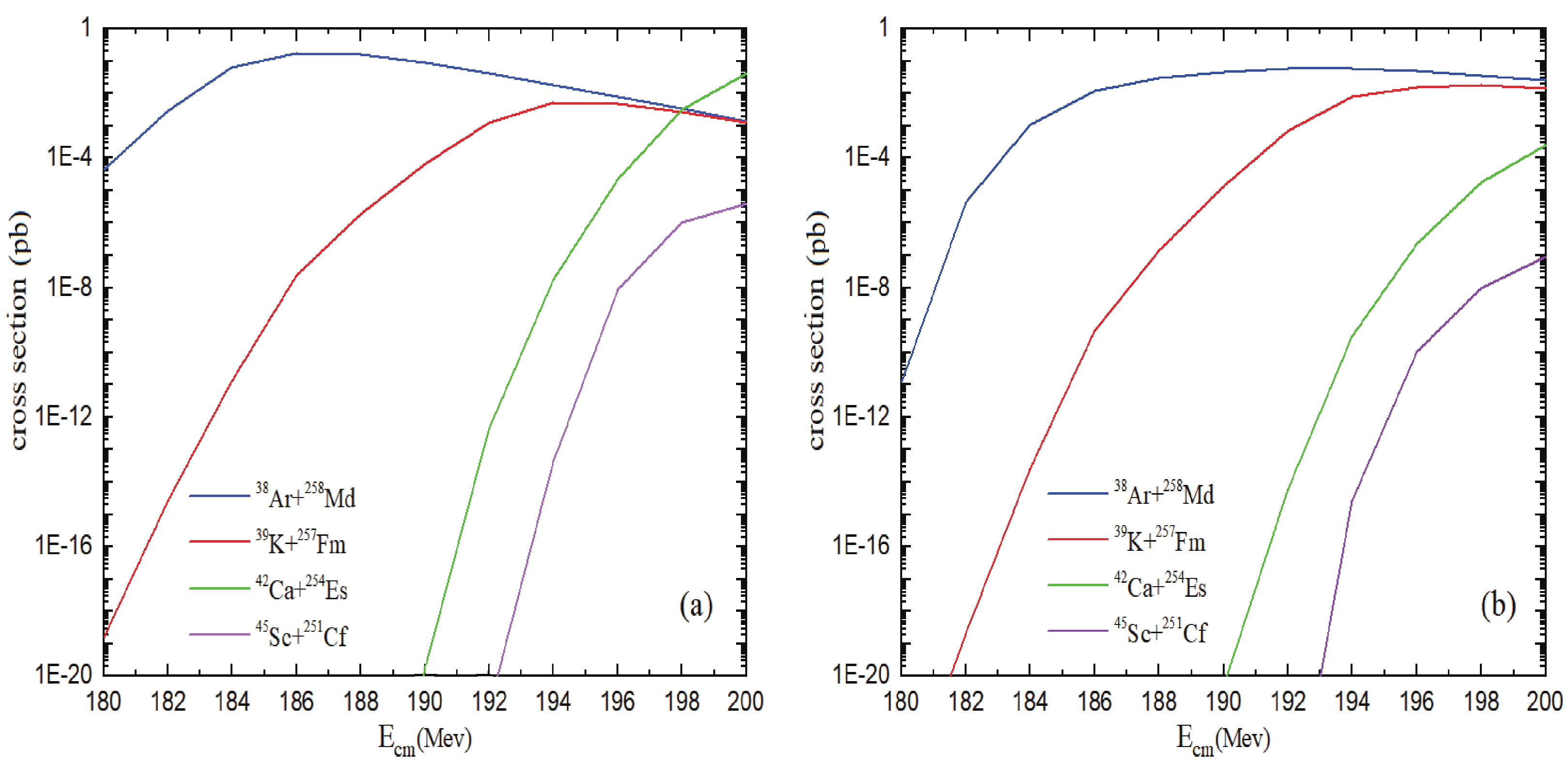Figure6. (color online) (a) Cross sections of the evaporation residue calculated for the 3n channel and (b) for the 4n channel in the reactions.

2 -->

D.Survival probability for the excited CN

For an excited CN, the probability to achieve a ground state with the emission of a neutron (or neutrons) is defined as “survival probability” and denoted by $W_{\rm sur}$ [39]. This probability computes the contest among particle evaporation in the $ xn, yp, z\alpha $ channel, the excited CN fission, and other particle evaporation channels [41, 42]. Therefore, the total survival cross section is the sum of the survival probability over all channels:

$ {\sigma}_{\rm surv}\left(E,l\right)=\pi { \lambda^{_{--}}}^2\mathop \sum \limits_{l = 0}^\infty {\left(2l+1\right)}T_l\left(E\right)P_{\rm CN}\left(E,l\right)\sum\limits_{xn,yp,z\alpha}W^{xn,yp,z\alpha}_{\rm surv}\left(E,l\right), $

(17)

Using the following equation, the survival probability for the 1n-evaporation channel is obtained:

$ W^{1n}_{\rm sur}(E_{\rm c.m.},J = 0) = \frac{\Gamma_n\left(E^*_{\rm CN}\right)}{\Gamma_f\left(E^*_{\rm CN}\right)} \\= \frac{4A^{{2}/{3}}\left(E^*_{\rm CN}-B_n\right)}{k\left(2{\left[a\left(E^*_{\rm CN}-B_f\right)\right]}^{{1}/{2}}-1\right)}\exp{\left[2a^{{1}/{2}}\left(\sqrt{E^*_{\rm CN}-B_n}-\sqrt{E^*_{\rm CN}-B_f}\right)\right]}, $

(18)

where k = 9.8 MeV and $E^*_{\rm CN} = E_{\rm c.m.}+Q$. Moreover, $ a = (A_1+ A_2)/{12} $ is the ratio for the level density, whose value in the evaporation channels is equal to one; $ B_f $ is the fission barrier for the heaviest nuclei, whose amount is proportional to the CN excitation energy ( $E_{\rm c.m.}$) as $B_f = B_f\left(E^*_{\rm CN}=0\right)\exp\left[-E^*_{\rm CN}/E_d\right]$, with $E_d=0.4A^{4/3}/a$ [3, 33, 34].
Previous studies showed that the probability of the survival is strongly proportional to the properties of the nuclear structure for the superheavy nuclei like deformation and level density [31]. We applied these properties in our calculations.
The results of calculation for $W_{\rm sur}$ and $ {\sigma }_{EvR} $ in the 1-4n channels (in the range of 180-200 MeV) for the $ {}^{38}_{18} $Ar + $ {}^{258}_{101} $Md reaction by using codes in Ref. [24] are shown in Fig. 7. According to this figure, the maximum value for $ {\sigma }_{EvR} $ at the 3n-channel and 4n-channel are 0.18 (pb) and 0.05 (pb), respectively, which is in good agreement with previously reported results [16-22] for the production of an element with 119 protons. The variety of results may be related to the various methods, potentials, energy range, and neutron numbers of the element.
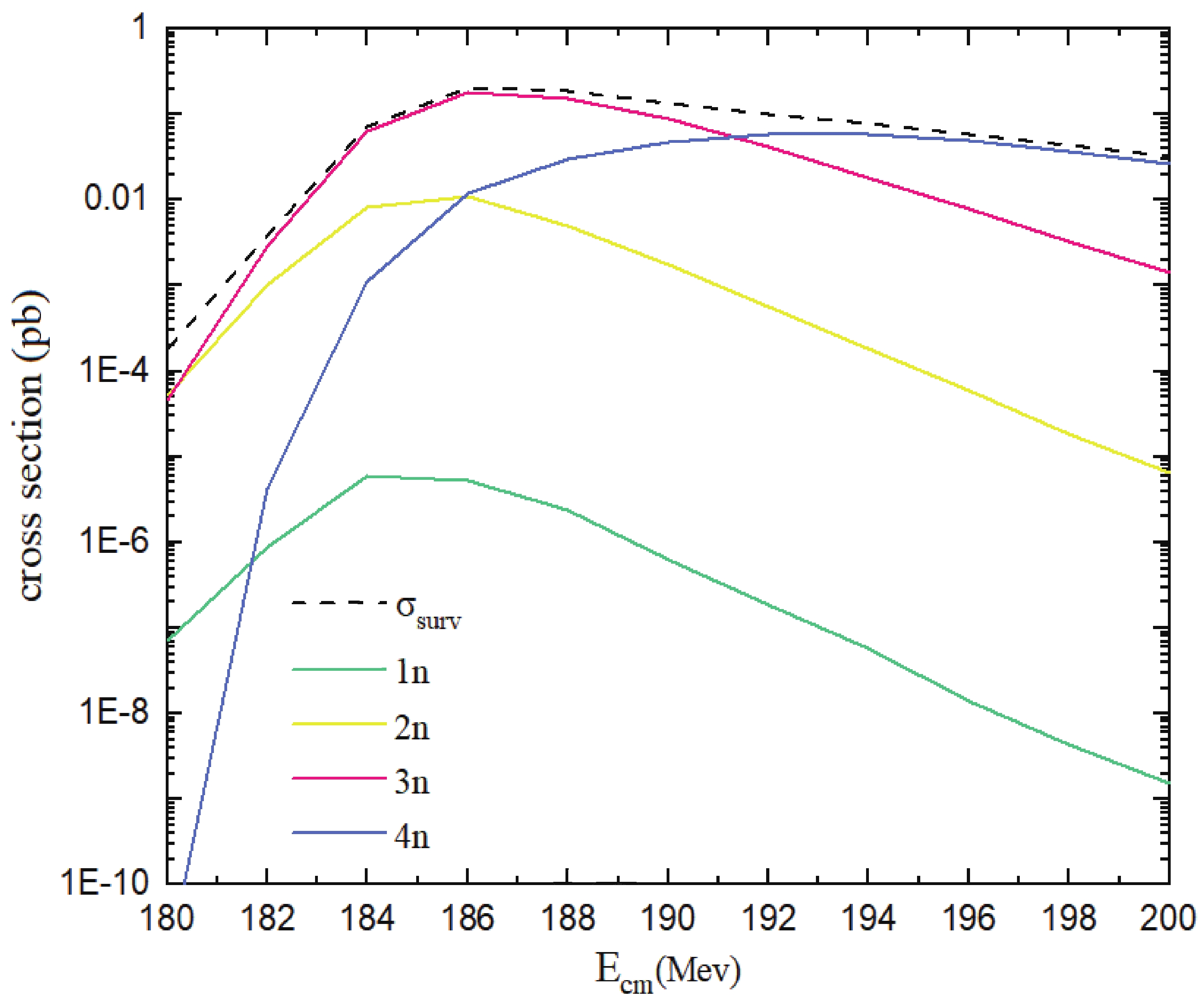Figure7. (color online) Survival cross section (dashed curve) and cross section of the evaporation residue (color curves) calculated for the 1n-4n channels in the $ {}^{38}_{18} $Ar + $ {}^{258}_{101} $Md reaction.

We used several codes available in Ref. [24] to study the formation of $ {}^{296} $119 superheavy compound nucleus at energies near the Coulomb barrier. Our calculations and studies lead to the following conclusions.
For the reactions with a larger mass asymmetry parameter, the minimum potential value in the contact point is further reduced. Thus, $ {}^{42}_{20} $Ca, $ {}^{39}_{19} $K, and $ {}^{38}_{18} $Ar, which are spherical and magic nuclei, have a greater amount than $ {}^{45}_{21} $Sc in the capture (even fusion) cross section and survival probability. For $ {}^{39}_{19} $K and $ {}^{38}_{18} $Ar, which have closed neutron shells, the survival probability for CN is greater than other studied reactions without closed neutron shells; however, for $ {}^{42}_{20} $Ca, which has closed proton shells, the CN survival probability is less than those of nuclei with closed neutron shells. Moreover, as the mass asymmetry parameter ($ \eta $) increases, the maximum values for the capture and fusion cross sections increase as well.
Although the maximum values for the capture and fusion cross sections are higher in the reaction $ {}^{38} $Ar + $ {}^{258} $Md, it is not accurate to conclude that this reaction is the optimal one among the mentioned four combinations just based on the fusion cross sections. This is because the excitation energy of the compound nucleus could be much higher, thereby suppressing the survival probability. However, this reaction is a suitable choice for the formation of an element with 119 protons among our studied reactions, because the calculated evaporation residue cross section in the $ {}^{38} $Ar + $ {}^{258} $Md reaction is larger than those of other reactions; moreover, this reaction has a smaller fusion barrier.