Yue Ding
, Zi-qiang Zhang ^,
,

Corresponding author: Zi-qiang Zhang, zhangzq@cug.edu.cn

School of Mathematics and Physics, China University of Geosciences, Wuhan 430074, China
Received Date:2020-08-09
Available Online:2021-01-15
Abstract:We perform a potential analysis for the holographic Schwinger effect in a deformed $ AdS_5 $ model with conformal invariance broken by a background dilaton. We evaluated the static potential by analyzing the classical action of a string attached to a rectangular Wilson loop on a probe D3 brane located at an intermediate position in the bulk AdS space. We observed that the inclusion of the chemical potential tends to enhance the production rate, which is opposite to the effect of the confining scale. In addition, we calculated the critical electric field based on the Dirac-Born-Infeld (DBI) action.

HTML

--> --> -->

The Schwinger effect is an interesting phenomenon in quantum electrodynamics (QED), by which virtual electron-position pairs can be materialized and become real particles owing to the presence of a strong electric field. The production rate $ \Gamma $ (per unit time and unit volume) was first calculated by Schwinger for weak-coupling and a weak-field in 1951 [1] as

$ \Gamma\sim \exp\left({\frac{-\pi m^2}{eE}}\right), $

(1)

where $ E $, $ m $, and $ e $ are the external electric field, electron mass, and elementary electric charge, respectively. In this case, there is no critical field trivially. Thirty-one years later, Affleck et al. generalized it to the case of arbitrary coupling and a weak-field [2] as

$ \Gamma\sim \exp\left({\frac{-\pi m^2}{eE}+\frac{e^2}{4}}\right), $

(2)

where the exponential suppression vanishes when $ E $ reaches $ E_c = (4\pi/e^3)m^2\simeq137m^2/e $. Clearly, the critical field $ E_c $ does not satisfy the weak-field condition, i.e., $ eE\ll m^2 $. Thus, it seems that one cannot determine $ E_c $ under the weak-field condition. In addition, one cannot determine whether a catastrophic decay actually occurs.
In fact, the Schwinger effect is not unique to QED but is a universal aspect of quantum field theories (QFTs) coupled to a U(1) gauge field. However, it remains difficult to study this effect in a QCD-like manner or through a confining theory using QFTs because the (original) Schwinger effect must be non-perturbative. Fortunately, the AdS/CFT correspondence [3-5] may provide an alternative approach. In 2011, Semenoff and Zarembo proposed [6] a holographic setup to study the Schwinger effect based on the Higgsed $ {\cal N} = 4 $ supersymmetric Yang-Mills theory (SYM). They found that at a large $ N $ and a large 't Hooft coupling $ \lambda $

$ \Gamma\sim \exp\left[-\frac{\sqrt{\lambda}}{2}\left(\sqrt{\frac{E_c}{E}}-\sqrt{\frac{E}{E_c}}\right)^2\right], \qquad E_c = \frac{2\pi m^2}{\sqrt{\lambda}}, $

(3)

Interestingly, the value of $ E_c $ coincides with that obtained from the DBI action [7]. Subsequently, Sato and Yoshida argued that [8] the Schwinger effect can be studied using a potential analysis. Specifically, the pair production can be estimated using a static potential, consisting of static mass energies, an electric potential from an external electric-field, and the Coulomb potential between a particle-antiparticle pair. The shapes of the potential depend on the external field $ E $ (see Fig. 1). When $ E<E_c $, the potential barrier is present, and the Schwinger effect can occur as a tunneling process. As $ E $ increases, the barrier decreases and gradually disappears at $ E = E_c $. When $ E>E_c $, the vacuum becomes catastrophically unstable. Further studies on the Schwinger effect in this direction can be found in [9-19]. The holographic Schwinger effect has also been investigated from the imaginary part of a probe brane action [20-23]. For a recent review on this topic, see [24].
Figure1. $ V(x) $ versus $ x $ with $ V(x) = 2m-eEx-\frac{\alpha_s}{x} $, where $ \alpha_s $ denotes the fine-structure constant.

Herein, we present an alternative holographic approach to study the Schiwinger effect using potential analysis. As the motivation of this study, holographic QCD models, such as hard walls [25,26], soft walls [27], and some improved AdS/QCD models [28-34] have achieved considerable success in describing various aspects of hadron physics. In particular, we will adopt the SW$ _{T,\mu} $ model [35], which is defined by the AdS with a charged black hole to describe the finite temperature and density multiplied by a warp factor to generate confinement. It turns out that such a model can provide a good phenomenological description of quark-antiquark interaction. In addition, the resulting deconfinement line in the $ \mu-T $ plane is similar to that obtained by lattice and effective models of QCD (for further studies on models of this type, see [36-41]). Motivated by this, in this study, we considered the Schwinger effect in the SW$ _{T,\mu} $ model. Specifically, we want to understand how the Schwinger effect is affected by the chemical potential and confining scale. In addition, this study can be considered as an extension of [8] to a case using the chemical potential and confining scale.
The outline of this paper is as follows. In the next section, we briefly review the SW$ _{T,\mu} $ model given in [35]. In Section III, we describe the potential analysis for the Schwinger effect in the SW$ _{T,\mu} $ model and investigate how the chemical potential and confining scale affect the production rate. In addition, we calculate the critical field from the DBI action. Finally, we provide some concluding remarks regarding our results in Section IV.

This section is devoted to a short introduction of the SW$ _{T,\mu} $ model proposed in [35]. The metric of the model in the string frame takes the following form:

$ {\rm d}s^2 = \frac{R^2}{z^2}h(z)\left(-f(z){\rm d}t^2+{\rm d}\vec{x}^{\,2}+\frac{{\rm d}z^2}{f(z)}\right), $

(4)

with

$ f(z) = 1-(1+Q^2)\left(\frac{z}{z_h}\right)^4+Q^2\left(\frac{z}{z_h}\right)^6, \qquad h(z) = {\rm e}^{c^2z^2}, $

(5)

where $ R $ is the AdS radius. Here $ Q $ represents the charge of a black hole; $ z $ denotes the fifth coordinate with $ z = z_h $ as the horizon, which is defined by $ f(z_h) = 0 $. The warp factor $ h(z) $, characterizing the soft wall model, distorts the metric and brings about a confining scale $ c $ (see [28] for an analytical way to introduce the warp factor through a potential reconstruction approach).
The temperature of the black hole is

$ T = \frac{1}{\pi z_h}\left(1-\frac{Q^2}{2}\right), \;\;\;\; 0\leqslant Q\leqslant \sqrt{2}. $

(6)

In addition, the chemical potential is

$ \begin{array}{l} \mu = \sqrt{3}Q/z_h. \end{array} $

(7)

Note that, for $ Q = 0 $, the SW$ _{T,\mu} $ model reduces to the Andreev model [42]. For $ c = 0 $, it becomes an AdS-Reissner Nordstrom black hole [43,44]. For $ Q = c = 0 $, it returns to an AdS black hole.

In this section, we follow the argument in [8] to study the behavior of the Schwinger effect in the SW$ _{T,\mu} $ model. Because the calculations of [8] were performed using the radial coordinate $ r = R^2/z $, for contrast, we also use coordinate $ r $.
The Nambu-Goto action is

$ S = T_F\int {\rm d}\tau {\rm d}\sigma{\cal L} = T_F\int {\rm d}\tau {\rm d}\sigma\sqrt{g}, \quad T_F = \frac{1}{2\pi\alpha^\prime}, $

(8)

where $ \alpha^\prime $ is related to $ \lambda $ by $ \frac{R^2}{\alpha^\prime} = \sqrt{\lambda} $, and $ g $ represents the determinant of the induced metric

$ g_{\alpha\beta} = g_{\mu\nu}\frac{\partial X^\mu}{\partial\sigma^\alpha} \frac{\partial X^\nu}{\partial\sigma^\beta}, $

(9)

where $ g_{\mu\nu} $ is the metric, and $ X^\mu $ is the target space coordinate.
Supposing the pair axis is aligned in one direction, e.g., the $ x_1 $ direction,

$ \begin{array}{l} t = \tau, \;\;\; x_1 = \sigma, \;\;\; x_2 = 0,\;\;\; x_3 = 0, \;\;\; r = r(\sigma). \end{array} $

(10)

Under this ansatz, the induced metric reads as follows:

$ \begin{aligned}[b]& g_{00} = \frac{r^2h(r)f(r)}{R^2}, \\& g_{01} = g_{10} = 0, \\&g_{11} = \frac{r^2h(r)}{R^2}+\frac{R^2h(r)}{r^2f(r)}\left(\frac{{\rm d}r}{{\rm d}\sigma}\right)^2, \end{aligned} $

(11)

and the Lagrangian density then becomes

${\cal L} = \sqrt{M(r)+N(r)\left(\frac{{\rm d}r}{{\rm d}\sigma}\right)^2}, $

(12)

with

$ M(r) = \frac{r^4h^2(r)f(r)}{R^4},\qquad N(r) = h^2(r). $

(13)

Because $ {\cal L} $ does not depend on $ \sigma $ explicitly, the Hamiltonian is conserved,

$ {\cal L}-\frac{\partial{\cal L}}{\partial\left(\dfrac{{\rm d}r}{{\rm d}\sigma}\right)}\left(\dfrac{{\rm d}r}{{\rm d}\sigma}\right) = {\rm Constant}. $

(14)

Imposing the boundary condition at the tip of the minimal surface,

$ \frac{{\rm d}r}{{\rm d}\sigma} = 0,\;\;\; r = r_c\;\;\; (r_t<r_c<r_0) , $

(15)

one gets

$ \frac{{\rm d}r}{{\rm d}\sigma} = \sqrt{\frac{M^2(r)-M(r)M(r_c)}{M(r_c)N(r)}} , $

(16)

with $ M(r_c) = M(r)|_{r = r_c} $. Here, $ r = r_t $ is the horizon, and $ r = r_0 $ is an intermediate position, which can yield a finite mass [6]. The configuration of the string world-sheet is depicted in Fig. 2.
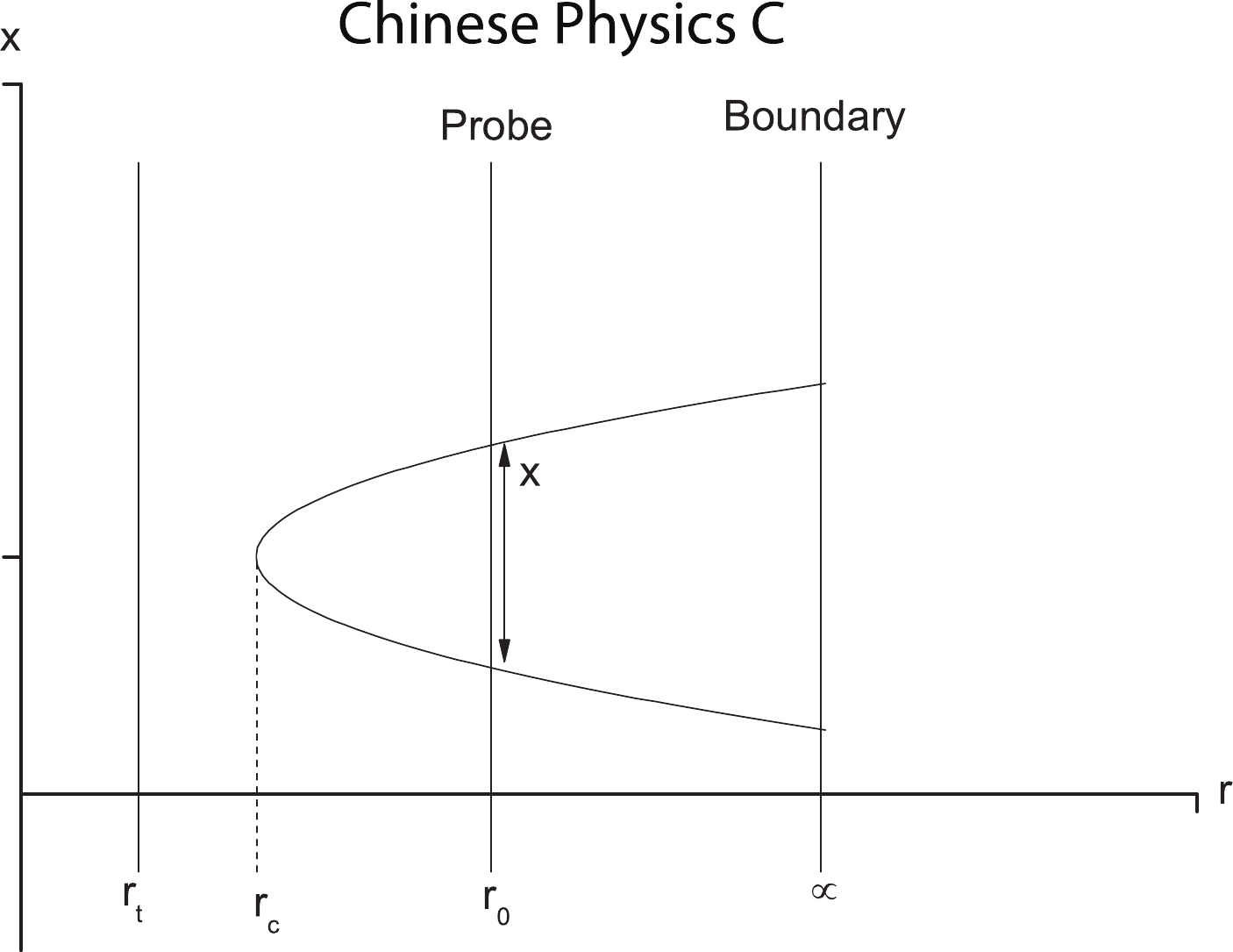Figure2. Configuration of string world-sheet.

Integrating (16) with the boundary condition (15), the following inter-distance of the particle pair is obtained:

$ x = 2\int_{r_c}^{r_0}\frac{{\rm d}\sigma}{{\rm d}r}{\rm d}r = 2\int_{r_c}^{r_0}{\rm d}r\sqrt{\frac{M(r_c)N(r)}{M^2(r)-M(r)M(r_c)}} . $

(17)

In contrast, plugging (12) into (8), the sum of the Coulomb potential and static energy is given by the following:

$ V_{CP+E} = 2T_F\int_{r_c}^{r_0}{\rm d}r\sqrt{\frac{M(r)N(r)}{M(r)-M(r_c)}}. $

(18)

The next task is to calculate the critical field. The DBI action is

$ S_{\rm DBI} = -T_{\rm D3}\int {\rm d}^4x\sqrt{-{\rm det}(G_{\mu\nu}+\mathcal{F}_{\mu\nu})} , $

(19)

with

$ T_{\rm D3} = \frac{1}{g_s(2\pi)^3\alpha^{\prime^2}}, \;\;\; \mathcal{F}_{\mu\nu} = 2\pi\alpha^\prime F_{\mu\nu}, $

(20)

where $ T_{D3} $ is the D3-brane tension.
The induced metric is

$ G_{00} = -\frac{r^2h(r)f(r)}{R^2}, \;\;\; G_{11} = G_{22} = G_{33} = \frac{r^2h(r)}{R^2}. $

(21)

Supposing the electric field is turned on along the $ x_1 $ direction [8],

$ \begin{array}{l} G_{\mu\nu}+\mathcal{F}_{\mu\nu} = \left( \begin{array}{cccc} -\dfrac{r^2h(r)f(r)}{R^2} & 2\pi\alpha^\prime E & 0 & 0\\ -2\pi\alpha^\prime E & \dfrac{r^2h(r)}{R^2} & 0 & 0 \\ 0 & 0 & \dfrac{r^2h(r)}{R^2} & 0\\ 0 & 0 & 0 & \dfrac{r^2h(r)}{R^2} \end{array} \right), \end{array} $

(22)

which results in

$ {\rm det}(G_{\mu\nu}+\mathcal{F}_{\mu\nu}) = \frac{r^4h^2(r)}{R^4}\left[(2\pi\alpha^\prime)^2E^2-\frac{r^4h^2(r)f(r)}{R^4}\right]. $

(23)

Substituting (23) into (19) and locating the probe D3-brane at $ r = r_0 $, one finds

$ S_{\rm DBI} = -T_{\rm D3}\frac{r_0^2h(r_0)}{R^2}\int {\rm d}^4x \sqrt{\frac{r_0^4h^2(r_0)f(r_0)}{R^4}-(2\pi\alpha^\prime)^2E^2} , $

(24)

with $ f(r_0) = f(r)|_{r = r_0} $, $ h(r_0) = h(r)|_{r = r_0} $.
To avoid (24) being ill-defined, one should get

$ \frac{r_0^4h^2(r_0)f(r_0)}{R^4}-(2\pi\alpha^\prime)^2E^2\geqslant 0, $

(25)

yielding

$ E\leqslant T_F\frac{r_0^2h(r_0)}{R^2}\sqrt{f(r_0)}. $

(26)

As a result, the critical field is as follows:

$ E_c = T_F\frac{r_0^2h(r_0)}{R^2}\sqrt{f(r_0)}, $

(27)

and it can be seen that $ E_c $ depends on $ T $, $ \mu $, and $ c $.
Next, we calculate the total potential. For simplicity, we introduce the following dimensionless parameters

$ \alpha\equiv\frac{E}{E_c}, \;\;\; y\equiv\frac{r}{r_c},\;\;\; a\equiv\frac{r_c}{r_0},\;\;\; b\equiv\frac{r_t}{r_0}. $

(28)

Given the above, the total potential reads as follows:

$ \begin{aligned}[b] V_{\rm tot}(x) = &V_{CP+E}-Ex = 2ar_0T_F\int_1^{1/a}{\rm d}y\sqrt{\frac{A(y)B(y)}{A(y)-A(y_c)}}\\& - 2ar_0T_F\alpha \frac{r_0^2h(y_0)}{R^2}\sqrt{f(y_0)}\\&\times \int_1^{1/a} {\rm d}y\sqrt{\frac{A(y_c)B(y)}{A^2(y)-A(y)A(y_c)}}, \end{aligned} $

(29)

with

$ \begin{aligned}[b]& A(y) = \frac{(ar_0y)^4h^2(y)f(y)}{R^4},\quad A(y_c) = \frac{(ar_0)^4h^2(y_c)f(y_c)}{R^4},\\& B(y) = h^2(y) ,\quad h(y) = {\rm e}^{\textstyle\frac{c^2R^4}{(ar_0y)^2}},\\& f(y) = 1-\left(1+\frac{\mu^2R^4}{3r_t^2}\right)\left(\frac{b}{ay}\right)^4+\frac{\mu^2R^4}{3r_t^2}\left(\frac{b}{ay}\right)^6, \\& h(y_c) = {\rm e}^{\textstyle\frac{c^2R^4}{(ar_0)^2}},\quad f(y_c) = 1-\left(1+\frac{\mu^2R^4}{3r_t^2}\right)\left(\frac{b}{a}\right)^4+\frac{\mu^2R^4}{3r_t^2}\left(\frac{b}{a}\right)^6,\\ &h(y_0) = {\rm e}^{\textstyle\frac{c^2R^4}{r_0^2}},\quad f(y_0) = 1-\left(1+\frac{\mu^2R^4}{3r_t^2}\right)b^4+\frac{\mu^2R^4}{3r_t^2}b^6, \end{aligned} $

(30)

we have checked that, by taking $ c = \mu = 0 $ in (29), the result of $ \mathcal{N} = 4 $ SYM [8] is regained.
Before going further, we should discuss the value of $ c $. In this study, we considered the behavior of the holographic Schwinger effect in a class of models parametrized by $ c $. To this end, we make $ c $ dimensionless by normalizing it at fixed temperatures and express other quantities in units of $ \mu $. In [45], the authors found that the range of $ 0\leqslant c/T\leqslant 2.5 $ is the most relevant for a comparison with QCD. We therefore use this range.
In Fig. 3, we plot $V_{\rm tot}(x)$ as a function of $ x $ for $ \mu/T = 1 $ and $ c/T = 0.1 $ (other cases with different values of $ \mu/T $ and $ c/T $ have a similarity), where we set $ b = 0.5 $ and $ T_Fr_0 = R^2/r_0 = 1 $ as in [8]. From these figures, it can be seen that a critical electric field exists at $ \alpha = 1 $ ($ E = E_c $), and for $ \alpha<1 $ ($ E<E_c $), the potential barrier is present, which is in agreement with [8].
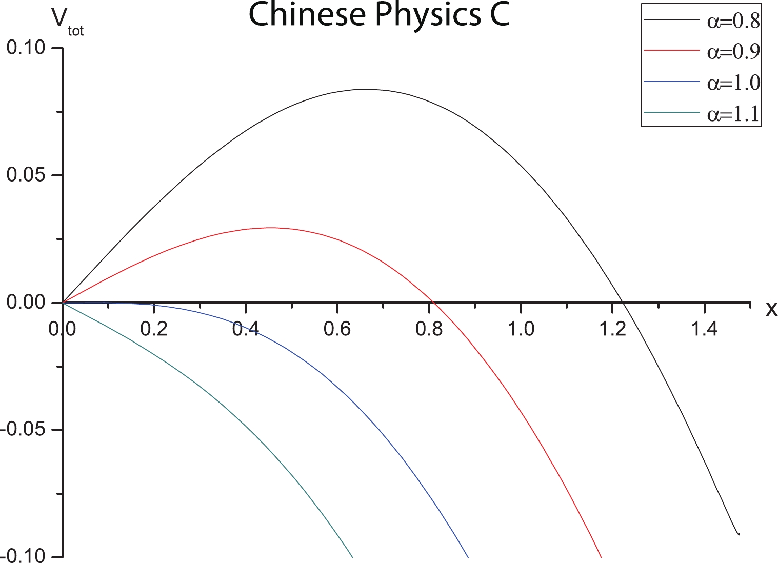Figure3. (color online) $ V_{\rm tot}(x) $ versus $ x $ with $ \mu/T = 1 $ and $ c/T = 0.1 $. In the plots, from top to bottom, $\alpha = 0.8,\; 0.9,\; 1.0,\; 1.1$, respectively.

To see how the chemical potential modifies the Schwinger effect, we plot $V_{\rm tot}(x)$ versus $ x $ with a fixed $ c/T $ for different values of $ \mu/T $ in Fig. 4. The left panel is for $ c/T = 0.1 $, and the right one is for $ c/T = 2.5 $. In both panels, from top to bottom, $ \mu/T = 0, 1, 5 $, respectively. One can see that, at a fixed $ c/T $, as $ \mu/T $ increases, both the height and width of the potential barrier decrease. As we know, the higher or wider the potential barrier is, the more difficult it is for the produced pairs to escape to infinity. Thus, it can be concluded that the inclusion of the chemical potential decreases the potential barrier, thus enhancing the Schwinger effect, in accordance with the findings of [14].
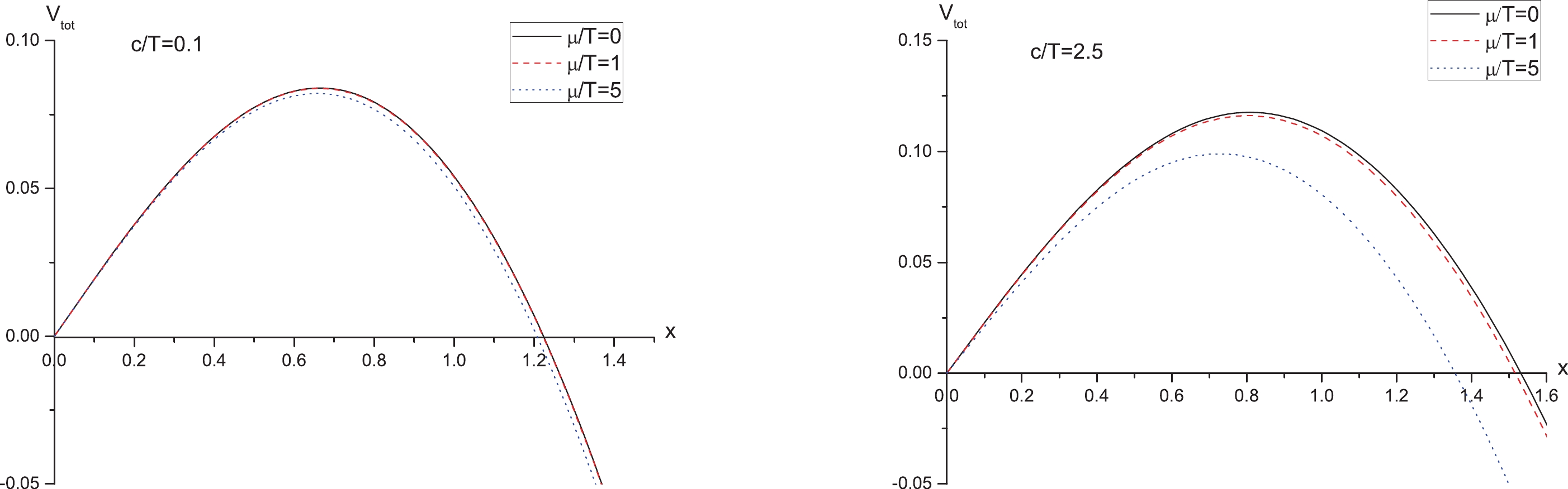Figure4. (color online) $ V_{\rm tot}(x) $ versus $ x $ with $ \alpha = 0.8 $ and fixed $ c/T $ for different values of $ \mu/T $. In both plots, from top to bottom, $ \mu/T = 0, 1, 5 $, respectively.

In addition, we plot $V_{\rm tot}(x)$ against $ x $ with a fixed $ \mu/T $ for different values of $ c/T $ in Fig. 5. It can be seen that, at a fixed $ \mu/T $, both the height and width of the potential barrier increase as $ c/T $ increases, implying that the presence of a confining scale reduces the Schwinger effect, inverse to the effect of the chemical potential.
Figure5. (color online) $ V_{\rm tot}(x) $ versus $ x $ with $ \alpha = 0.8 $ and fixed $ \mu/T $ for different values of $ c/T $. In both plots, from top to bottom, $ c/T = 2.5, 1, 0 $, respectively.

Finally, to understand how the chemical potential and confining scale affect the critical electric field, we plot $ E_c/E_{c0} $ versus $ \mu/T $ ($ c/T $) in the left (right) panel of Fig. 6, where $ E_{c0} $ denotes the critical electric field of the SYM. It can be seen that $ E_c/E_{c0} $ decreases as $ \mu/T $ increases, indicating that the chemical potential decreases $ E_c $, thus enhancing the Schwinger effect. Meanwhile, the confining scale has an opposite effect, consistent with the potential analysis. Furthermore, it can be seen that $ E_c/E_{c0} $ can be larger or smaller than 1, which means that the SW$ _{T,\mu} $ model may provide a wider range of the Schwinger effect in comparison to SYM.
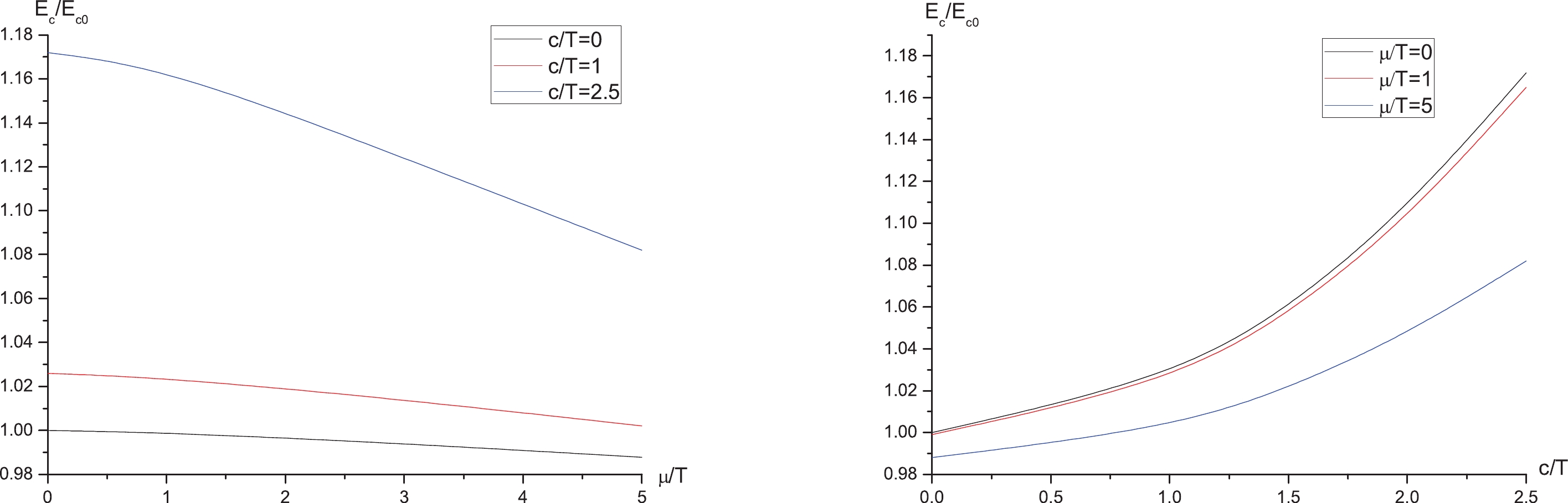Figure6. (color online) Left: $ E_c/E_{c0} $ versus $ \mu/T $; from top to bottom, $ c/T = 2.5, 1, 0 $, respectively. Right: $ E_c/E_{c0} $ versus $ c/T $; from top to bottom, $ \mu/T = 0, 1, 5 $, respectively.

The study of the Schwinger effect in non-conformal plasma under the influence of the chemical potential may shed some light on heavy ion collisions. In this paper, we investigated the effect of the chemical potential and confining scale on the holographic Schwinger effect in a soft wall AdS/QCD model. We analyzed the electrostatic potentials by evaluating the classical action of a string attached to the rectangular Wilson loop on a probe D3 brane located at an intermediate position in the bulk AdS and calculated the critical electric field from the DBI action. We found that the inclusion of the chemical potential tends to decrease the potential barrier, thus enhancing the production rate, opposite to the effect of the confining scale. Moreover, we observed that, with some chosen values of $ \mu/T $ and $ c/T $,$ E_c $ can be larger or smaller than the counterpart in SYM, implying that the SW$ _{T,\mu} $ model may provide a theoretically wider range of the Schwinger effect in comparison to SYM.
However, there are some questions that need to be addressed further. First, the potential analysis is basically within the Coulomb branch, related to the leading exponent corresponding to the on-shell action of the instanton and not the full decay rate. In addition, the SW$ _{T,\mu} $ model is not a consistent model because it does not solve the full set of equations of motion. Performing such an analysis in some consistent models, e.g., those in [28-34], would be instructive (usually the metrics of such models are only known numerically, and thus, the calculations are more challenging).