Qi Li ^1,
, Jing Li ^1,
, Yongxiang Zhou ^1,
, Xun Xue ^1,2,,
,

Corresponding author: Xun Xue, xxue@phy.ecnu.edu.cn

1.Department of Physics, East China Normal University, Shanghai 200241, China
2.Center for Theoretical Physics, Xinjiang University, Urumqi 830046, China
Received Date:2020-03-20
Accepted Date:2020-06-20
Available Online:2020-10-01
Abstract:The effective vacuum energy density contributed by the non-trivial contortion distribution and the bare vacuum energy density can be viewed as the energy density of the auxiliary quintessence field potential. We find that the negative bare vacuum energy density from string landscape leads to a monotonically decreasing quintessence potential while the positive one from swampland leads to the metastable or stable de Sitter-like potential. Moreover, the non-trivial Brans-Dicke like coupling between the quintessence field and gravitation field is necessary in the latter case.

HTML

--> --> -->

String theory is believed to be one of the candidates for the theories of quantum gravity. The reduction from string theory to the low energy field theory relies on the choice of possible ways of string vacua compactification, which can be of order $ 10^{500} $ and makes the string theory lack prediction power. The string vacua that preserve supersymmetry generally posses a negative energy density and hence are the anti-de Sitter (AdS) ones. However, one needs to increase the vacuum energy to positive values (see the illustrations in Figs. 1(a) and 1(b)) to explain the increase in the rate of inflation and the late-time accelerated expansion of the universe, e.g., by the KKLT construction [1]. The second criterion of swampland conjecture excludes the effective field theory (EFT) with a meta-stable dS vacuum as a theory possessing ultraviolet (UV) completion [2, 3] and leaves the quintessence type of potential as the only possible one to account for the evolution of the universe.
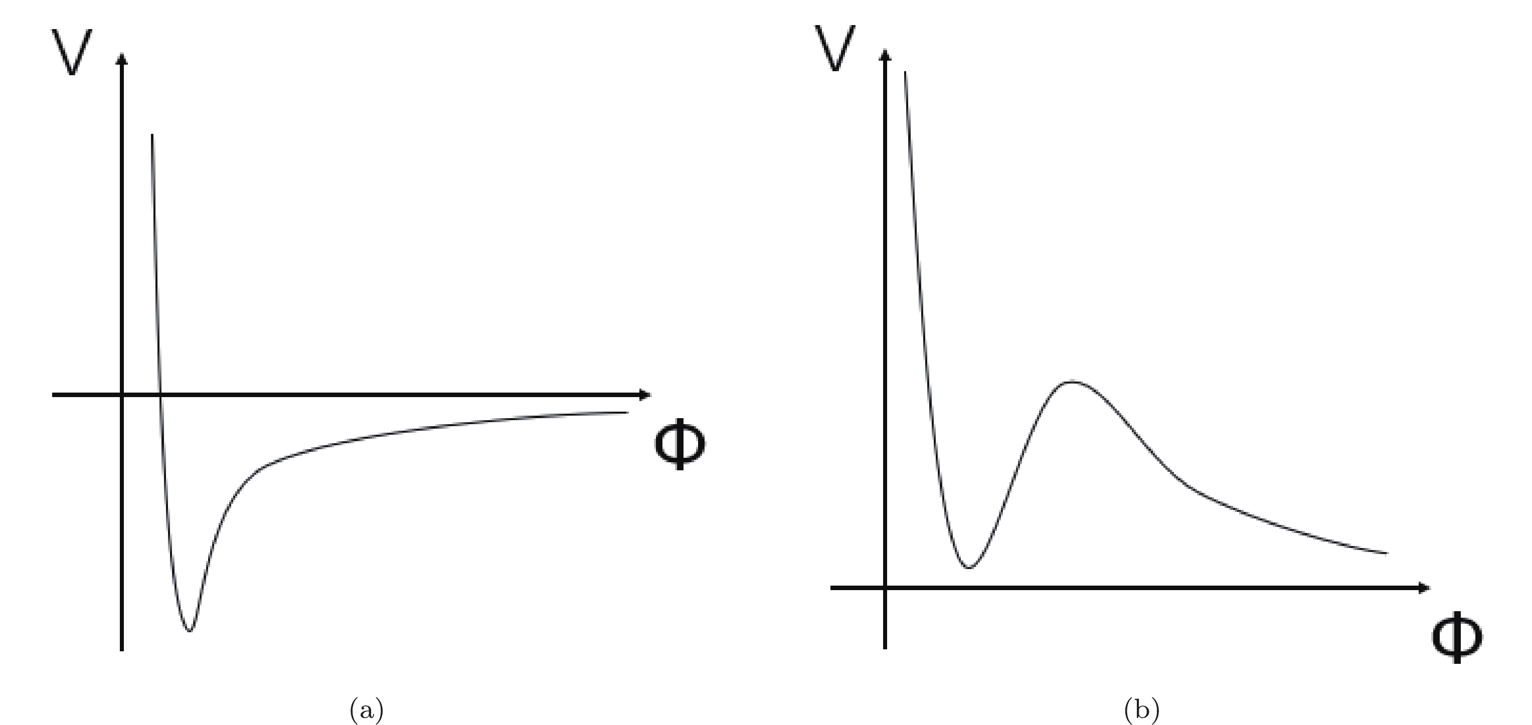Figure1. Illustrations of (a) the AdS vacuum and (b) the metastable dS vacuum.

Recently, an alternative construction to lift the AdS vacua to the de Sitter (dS) type has been proposed by utilizing the frozen large-scale Lorentz violation, which results in the contortion distribution at the cosmic scale [4, 5]. It has been pointed out that the possible Lorentz violation in quantum gravity during the era dominated by quantum gravity before inflation may be frozen by inflation. The scale of the Lorentz-violating area may stretch beyond the horizon [6, 7], and it may be transformed into a cosmic one even when the scale reenters the horizon during the late-time expansion. Dark energy may be an emergent effect of the large-scale Lorentz-violating effective gravity at the cosmic scale [7], in constrast with many proposed candidates for dark energy, ranging from the cosmological constant model to dynamic dark energy models such as the quintessence model [8].
In the quintessence model, it is supposed that the spacetime of the universe is dominated by an auxiliary scalar, namely quintessence, a field with the potential decreasing in magnitude as the value of the scalar field increases, as indicated in Fig. 2. Although the quintessence model successfully describes the late-time accelerating expansion of the universe, its origin is somewhat ambiguous. Is it fundamental or an effective description of some other quantities which are more original within the framework of fundamental physics? In this paper, the effective vacuum energy contributed by the bare cosmological constant and contortion defined in [4, 5] is effectively described using the quintessence field potential energy.
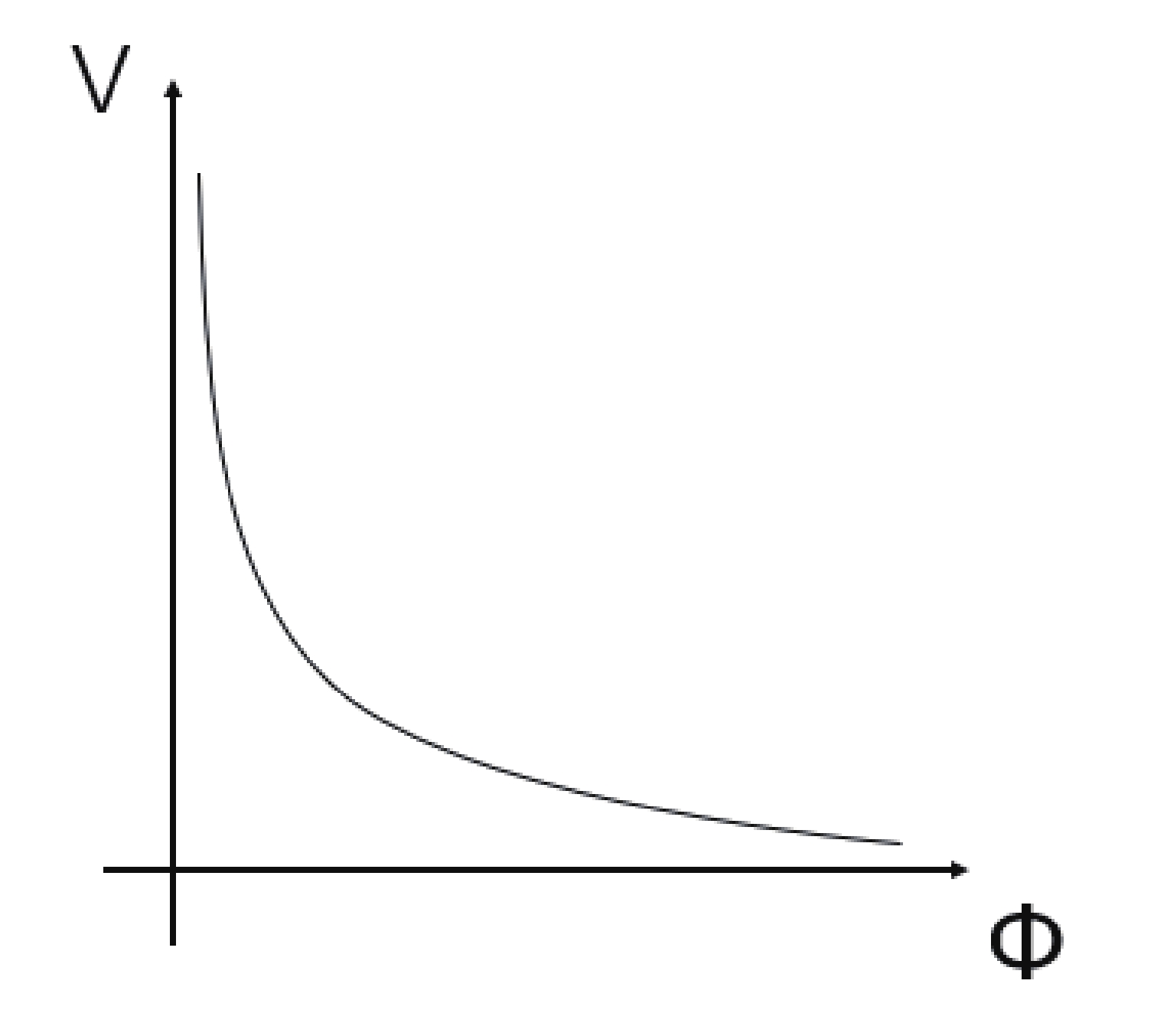Figure2. The monotonically decreasing quintessence potential can meet the requirement of the swampland conjecture and the accelerating expansion of the universe.

The evolution of the effective vacuum energy density proposed by Zhai et al. [4, 5] shows a transition from monotonically decreasing behavior when the bare vacuum energy density comes from string landscape to the existence of a local minimum with one from swampland. The result seems to be consistent with the requirement by the second criterion in swampland conjecture. However, the equivalent behavior between the evolution of effective vacuum energy density and the potential of an auxiliary field such as the quintessence field is not obvious.
In contrast with the conventional quintessence model, we consider that the quintessence field may interact with gravity in a non-minimal way, e.g., the Brans-Dicke coupling, in general. We repeat the similar basic picture given in [4], that is, there is a transition for the quintessence potential from monotonically decreasing to the meta-stable or stable de Sitter one, which possesses a local minimum when the bare vacuum energy density varies from negative as in the landscape to positive as in swampland. Moreover, we find that the non-trivial Brans-Dicke coupling between the quintessence field and gravity is necessary in the swampland case.

The effective gravitation theory with a large-scale Lorentz violation can be realized by introducing a gauge-fixing constraint to the Hilbert-Einstein theory. The constraint terms in the action supply an effective spin angular momentum distribution to the equations of motion for connection even in the case of a scalar matter source. The connection is thus with torsion in general and differs from the Levi-Civita one in the contortion part. The contortion part in turn contributes an effective energy-momentum distribution to the equations of motion for the metric tensor, the modified Einstein equations, with the Einstein tensor being composed purely of the Levi-Civita connection on the left-hand side of the equations and the organization of the terms involving contortion and the bare cosmological constant to the right-hand side of the equations [6, 7, 9-11]. Taking the possible cosmic-scale Lorentz boost violation into account, the modification to the Einstein equations entails the dark partner energy-momentum contribution from contortion in addition to the matter source one [7],

$ \widetilde{R}_{\ c}^{a}-\frac{1}{2}\delta_{\ c}^{a}\widetilde{R} = 8\pi G\left( T+T_{\Lambda}\right)_{\ c}^{a} \;, $

(1)

where $ \widetilde{R}_{\ c}^{a} $ is the Ricci tensor in Levi-Civita connection and $ T_{\Lambda} $ is the dark partner contribution of energy-momentum tensor, $ [T_{\Lambda}]_{\ c}^{a} = {\rm diag}(\rho_{\Lambda}, -p_{\Lambda}, -p_{\Lambda}, -p_{\Lambda}) $. The energy density $ \rho_{\Lambda} $ and pressure $ p_{\Lambda} $ can be expressed as

$ \rho_{\Lambda} = -\dfrac{c^4}{8\pi G}(3{\cal{K}}^2+6{\cal{K}}\dfrac{\dot{a}}{a}-\Lambda_0), $

(2)

and

$ p_{\Lambda} = -\dfrac{c^4}{8\pi G}({\cal{K}}^2+4{\cal{K}}\dfrac{\dot{a}}{a}+2\dot{{\cal{K}}}-\Lambda_0), $

(3)

respectively, where $ {\cal{K}}(t) = {K^0}_{11} = {K^0}_{22} = {K^0}_{33} $, the only non-zero components of contortion in a Robertson-Walker solution ansatz for the metric tensor of a uniform and isotropic universe in the comoving frame, and $ \Lambda_0 $ is the bare cosmological constant from vacuum energy density. $ \Lambda $ denotes the cosmological constant fitted from observation with $ \Lambda {\rm CDM} $ model, and $ x = \dfrac{\Lambda_{0}}{\Lambda} $. The modified Friedmann Equation in geometrical unit $ \dfrac{c^4}{8G\pi} = 1 $ can be written as [7],

$ {\cal{K}}^2 + 2{\cal{K}}\dfrac{\dot{a}}{a} +\left( \dfrac{\dot{a}}{a}\right) ^2 = \dfrac{1}{3}\left( \rho+\Lambda_{0}\right), $

(4)

and

$ \ddot{a} = -\frac{a}{2}\left( p+\dfrac{\rho}{3}\right) +\dfrac{1}{3}a\Lambda_{0}-\dfrac{\rm d}{{\rm d}t}\left( a{\cal{K}}\right), $

(5)

or

$\begin{split} \dot{H}(t)&+\dot{{\cal{K}}}(t)+H(t)\left[ H(t)+{\cal{K}}(t)\right]\\&+\dfrac{3w+1}{2}\left[ H(t)+{\cal{K}}(t)\right] ^2-\dfrac{w+1}{2}\Lambda_{0} = 0, \end{split} $

(6)

utilizing the equation of state for cosmic media $ p = w\rho $.
As discussed in reference [7], the equations of motion for $ {\cal{K}}(t) $ give an expression $ \left(f_t,f_r,f_\theta,f_\varphi\right) = \left(a(t){\cal{K}}(t)+ \dot a(t)\right)\cdot\left(0, \dfrac{1}{\sqrt{1-kr^2}}, r, r\sin\theta\right) $, where $ f_{\mu}(x) $ is introduced in the constrain equation $ \left({A^{0}}_{1\mu}\right)^2+\left({A^{0}}_{2\mu}\right)^2+ \left({A^{0}}_{3\mu}\right)^2 = \left(f_\mu (x)\right)^2 $ as a measure of Lorentz violation. In principle, $ f_{\mu}(x) $ can be derived from the fundamental theory of quantum gravity and specific model of inflation. However, to account for the late time accelerating expansion of the universe in a phenomenological view of point, it is a compromise to use some approximations to substitute the equations of motion for $ {\cal{K}}(t) $.
The evolution of $ {\cal{K}}(t) $ can be fixed by three kinds of approximations utilizing one independent equation among the Friedmann equations in the $ \Lambda {\rm CDM} $ model or the equation of state for dark partner part, in order to close the set of equations in addition to the modified Friedmann equations. The three approximations are Case A with additional equation

$ \dot{{\cal{K}}} = \dfrac 13\Lambda_0-\dfrac 13\Lambda-H{\cal{K}}\;\;, $

(7)

Case B with

$ \dot{{\cal{K}}}+(3w+2)H{\cal{K}}+\dfrac {3w+1}2{\cal{K}}^2 = \frac {w+1}2(\Lambda_0-\Lambda), $

(8)

and Case C with

$ (3w_0+1){\cal{K}}^2+(6w_0+4)H{\cal{K}}+2\dot{{\cal{K}}} = (w_0+1)\Lambda_0, $

(9)

where $ p_{\Lambda} = w_0\rho_{\Lambda} $ [7].
The initial value of $ {\cal{K}}(t) $ is obtained in a similar way,

$ {\cal{K}}(t_0) = H_0\left( \pm\sqrt{1-\dfrac{\Lambda-\Lambda_{0}}{3H_0}}-1\right), $

(10)

and hence a constraint is set for the value of $ \Lambda_0$

$ \Lambda_{0}\geqslant-(3H_0-\Lambda)\approx-\dfrac{2}{5}\Lambda \;. $

(11)

The evolution of the effective cosmological constant or the energy density of the dark partner,

$ \Lambda_{\rm eff} = \Lambda_0-3\left({\cal{K}}^2+2{\cal{K}}\dfrac{\dot{a}}{a}\right)\;\;, $

(12)

exhibits that there is a critical value for $ \Lambda_0 $, which separates the monotonically decreasing $ \Lambda_{\rm eff} $ phase from one with a local minimum. The critical value $ \Lambda_{\rm crit} \approx 0 $ is the division of vacuum energy density from landscape and swampland [5], as is indicated in Figs. 3 and 4.
Figure3. (color online) The transition of $ \Lambda_{\rm eff}$ from a monotonically decreasing quintessence phase to a phase with local minimum in case of $ {\cal{K}}(t_0)=H_0\left( \sqrt{1-\dfrac{\Lambda-\Lambda_{0}}{3H_0}}-1\right) $ in [5].

Figure4. (color online) The transition of $ \Lambda_{\rm eff}$ from a monotonically decreasing quintessence phase to a phase with local minimum in case of $ {\cal{K}}(t_0)=H_0\left( -\sqrt{1-\dfrac{\Lambda-\Lambda_{0}}{3H_0}}-1\right) $ in [5].

In the quintessence model, the dark energy energy-momentum tensor is described by the one contributed by the quintessence field [8]. If the quintessence field is regarded as an effective description of the contortion effect caused by large scale Lorentz violation, $ \Lambda_{\rm eff} $, the energy density of the dark partner can be represented by the energy density produced by the quintessence field. Consider a model of gravity involving non-minimal Brans-Dicke type of coupling between gravity and the quintessence field,

$\begin{split} S =& \int {\rm d}^4x\sqrt{-g}\left[\frac 12M^2_{pl}R\left( 1+\xi\phi^2\right)\right. \\&\left.-\frac 12g^{\mu\nu}\partial_{\mu}\phi\partial_{\nu}\phi-V(\phi)\right]+S_m \;, \end{split}$

(13)

where $ M_{pl} $ is the reduced Planck mass, R is the Ricci scalar, $ \xi $ is the non-minimal coupling constant between gravity and quintessence field, and $ S_m $ is the matter action. The equations of motion for gravity and scalar field are

$ \left( 1+\xi\phi^2\right) \left( R_{\mu\nu}-\frac{1}{2}g_{\mu\nu}R\right) = 8\pi GT_{\mu\nu}, $

(14)

and

$ V_{,\phi}+3H\dot{\phi}+\ddot{\phi}-M_{pl}^2R\xi\phi = 0, $

(15)

respectively. The pressure and energy density of the quintessence are given by $ P_{\phi} = \left[ \dot{\phi}^2/2-V(\phi)\right] /(1+\xi\phi^2) $ and $ \rho_{\phi} = \left[ \dot{\phi}^2/2+V(\phi)\right] /(1+\xi\phi^2) $, respectively. In an effective description of the dark partner energy density by quintessence field, we have

$ \Lambda_{\rm eff} = \rho_{\phi} = \frac {\dot{\phi}^2+2V(\phi)}{2+2\xi\phi^2}, $

(16)

or

$ \dot{\Lambda}_{\rm eff}\left( 1+\xi\phi^2\right)+2\Lambda_{\rm eff}\xi\phi\dot{\phi}+3H\dot{\phi}^2-M_{pl}^2R\xi\phi\dot{\phi} = 0, $

(17)

by Eq. (15), where the metric is assigned with the Robertson-Walker metric in the form of $ {\rm d}s^2 = -{\rm d}t^2+ a^2(t)\left({\rm d}r^2+ r^2{\rm d}\Omega^2\right) $. Formally, we have

$\begin{split} \dot{\phi} =& M_{pl}^2\xi\phi\left( \dfrac{\dot{H}}{H}+2H\right)-\dfrac{\Lambda_{\rm eff}\xi\phi}{3H}\\&\pm\sqrt{\left[ M_{pl}^2\xi\phi\left( \dfrac{\dot{H}}{H}+2H\right)-\dfrac{\Lambda_{\rm eff}\xi\phi}{3H}\right]^2-\dfrac{\dot{\Lambda}_{\rm eff}}{3H}\left( 1+\xi\phi^2\right) } \;, \end{split}$

(18)

which gives a constrain on the Brans-Dicke coupling $ \xi $ as

$ \left[3M_{pl}^2\left(\dot{H}+2H^2\right)-\Lambda_{\rm eff}\right]^2\phi^2\xi^2-3H\dot{\Lambda}_{\rm eff}\phi^2\xi-3H\dot{\Lambda}_{\rm eff}\geqslant 0 \;. $

(19)

The minimal values of the Brans-Dicke coupling constant $ \xi_{\rm min} $ in all cases during matter domination with $ w = 0 $ are plotted in Fig. 5 and Fig. 6. It reveals that the non-trivial Brans-Dicke type of coupling is necessary when $ \Lambda_0 $ exceeds a critical value in every case.
Figure5. (color online) The cases of initial value $ {\cal{K}}(t_0) = \sqrt{1-(\Lambda-\Lambda_0)/3H_0^2}-H_0 $ revealing the non-triviality of the non-minimal coupling, $ \xi_{\rm min}>0 $, when $ \Lambda_0>\Lambda_{\rm crit} $.

Figure6. (color online) The cases of initial value $ {\cal{K}}(t_0) = -\sqrt{1-(\Lambda-\Lambda_0)/3H_0^2}-H_0 $ revealing the non-triviality of the non-minimal coupling, $ \xi_{\rm min}>0 $, when $ \Lambda_0>\Lambda_{\rm crit} $.

The numerical calculation of Eq. (18) with plus sign gives the evolution of $ \phi $, a monotonical evolution versus t, as is shown in Fig. 7 and Fig. 8. The field $ \phi $ may thus be regarded as an intrinsic time for the evolution of the universe. The evolution of $ V(\phi) $ versus $ \phi $ is shown in Fig. 9 and Fig. 10. The critical value for $ \Lambda_{0} $ which symbolizes the transformation of $ V(\phi) $ from a monotonical quintessence like to the meta-stable dS potential is almost the same as one for $ \Lambda_{\rm eff}(t) $ in [5] in most cases.
Figure7. (color online) The monotonic evolution of $ \phi(t) $ in cases with initial value $ {\cal{K}}(t_0) = H_0( \sqrt{1-(\Lambda-\Lambda_{0})/3H_0}-1) $.

Figure8. (color online) The monotonic evolution of $ \phi(t) $ in cases with $ {\cal{K}}(t_0) = H_0( -\sqrt{1-(\Lambda-\Lambda_{0})/3H_0}-1) $.

Figure9. (color online) $ V(\phi) $ shifts from a monotonically decreasing quintessence phase to a dS one with a local minimum versus $ \phi $ evolution in cases of $ {\cal{K}}(t_0) = H_0( \sqrt{1-(\Lambda-\Lambda_{0})/3H_0}-1) $.

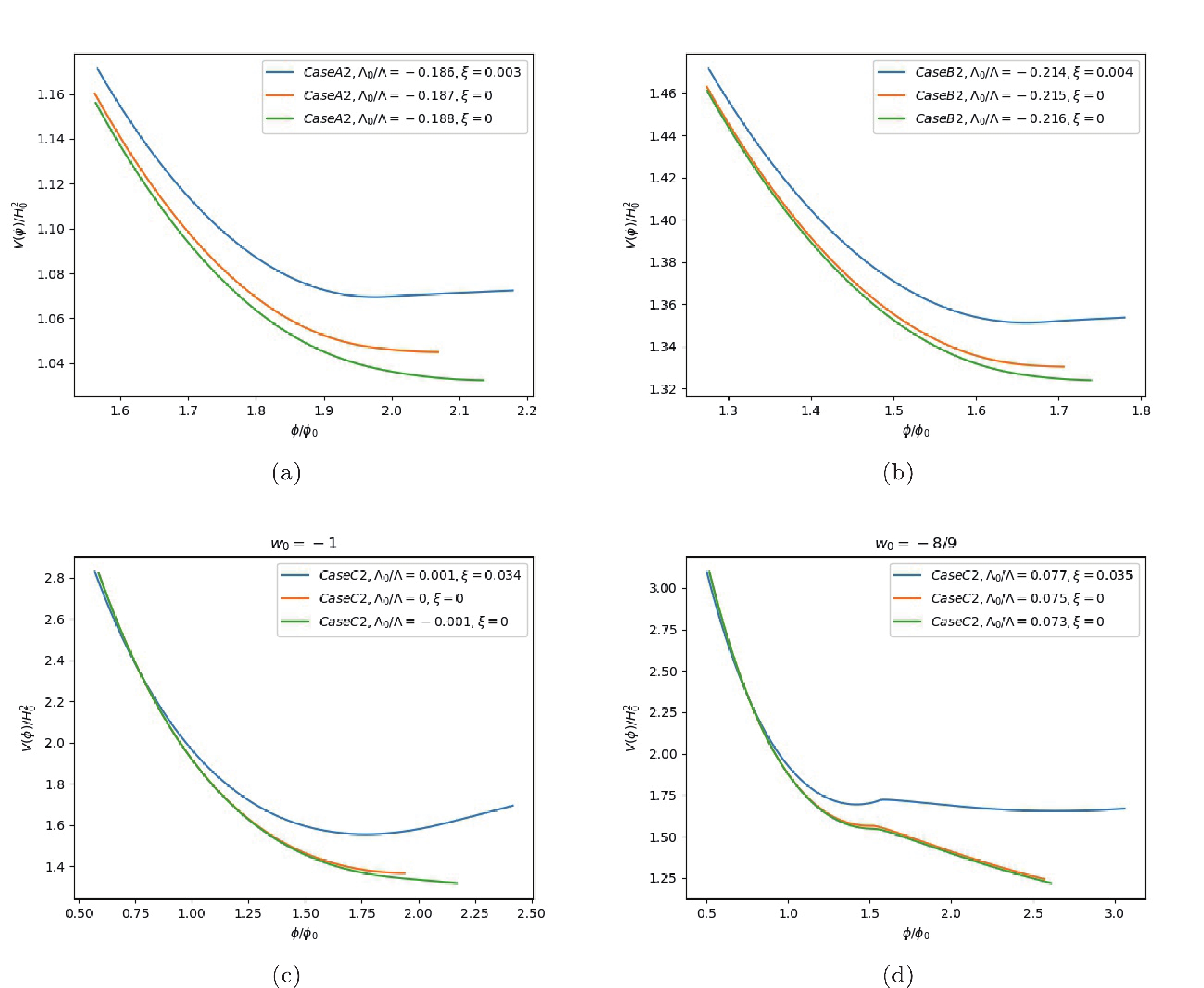Figure10. (color online) $ V(\phi) $ shifts from a monotonically decreasing quintessence phase to a dS one with a local minimum versus $ \phi $ evolution in cases of $ {\cal{K}}(t_0) = H_0( -\sqrt{1-(\Lambda-\Lambda_{0})/3H_0}-1) $.

It is a universal conclusion that the minimal Brans-Dicke coupling is non-trivial, i.e., $ \xi_{\rm min}>0 $, in all the cases when $ \Lambda_0>\Lambda_{\rm crit} $. Note that the minimal value of the coupling constant satisfies

$ \dot{\Lambda}_{\rm eff} = \dfrac{\dot{\phi}\left( \ddot{\phi}+V_{,\phi}-2\xi\phi\Lambda_{\rm eff}\right) }{1+\xi\phi^2} = \dfrac{\dot{\phi}\left[ \left( M^2_{pl}R-2\Lambda_{\rm eff}\right)\xi\phi-3H\dot{\phi} \right] }{1+\xi\phi^2}, $

(20)

from Eq. (19), in the increasing region of $ V(\phi) $ when $ \Lambda_0>\Lambda_{\rm crit} $, $ \dot{\Lambda}_{\rm eff}>0 $ implies that

$ \left( M^2_{pl}R-2\Lambda_{\rm eff}\right)\xi\phi-3H\dot{\phi} \geqslant 0 \;. $

(21)

At the minimum of $ V(\phi) $, it holds that

$ M^2_{pl}R-2\Lambda_{\rm eff} > 0, $

(22)

i.e.

$ \xi\geqslant \dfrac{3H\dot{\phi}}{\left(M^2_{pl}R-2\Lambda_{\rm eff}\right)\phi} \;. $

(23)

As pointed out in [5], the Case C approximation is not suitable from the comparison between Hubble constant versus time and the luminosity distance versus redshift z. The reason may be that a fixed $ w_0 $ in the equation of state of dark partner part is assumed. The case $ w_0>-8/9 $ can be ignored (excluded by observation of luminosity distance with redshift relation [5]), we can conclude that the meta-stable dS potential needs non-trivial coupling between quintessence field and gravitation. The conclusion that quintessence potential can be generated from string landscape AdS vacuum effectively and the critical value of cosmological constant separating quintessence from meta-stable dS is approximately zero still holds for the effective description of quintessence field theory.
The discussion on the non-triviality of $ \xi_{\rm min} $ can be easily extended to the case including radiation and warm dark matter. We show the numerical results for $ \xi_{\rm min} $ values for all the cases with w ranging from $ 1/3 $ to $ 0 $ in Tables 1, 2, 3, and 4. The second column of the tables for both cases, which correspond to the critical value $ \Lambda_{\rm crit} $ reveal that the dependence of starting point for non-trivial $ \xi_{\rm min} $ on w is insensitive; a similar conclusion can be drawn from the numerical results for w ranging from $ 1/3 $ to $ 0 $ as that for the $ w = 0 $ case.

	$\xi_{\rm min}$ for Case A1($x_{\rm crit}=-0.05$)					$\xi_{\rm min}$ for Case A2($x_{\rm crit}=-0.187$)
	x=?0.1	x=?0.05	x=0	x=0.1		x=?0.2	x=?0.186	x=?0.1	x=0.1
$ w=0 $	0	0	0.135	0.249		0	0.003	0.111	0.391
$ w=1/24 $	0	0.029	0.142	0.255		0	0	0.114	0.401
$ w=1/12 $	0	0.041	0.152	0.261		0	0	0.115	0.412
$ w=1/8 $	0	0.05	0.155	0.268		0	0	0.114	0.422
$ w=1/6 $	0	0.057	0.161	0.274		0	0	0.109	0.432
$ w=5/24 $	0	0.063	0.167	0.28		0	0	0.099	0.442
$ w=1/4 $	0	0.069	0.173	0.284		0	0	0.076	0.452
$ w=7/24 $	0	0.074	0.178	0.291		0	0	0	0.461
$ w=1/3 $	0	0.078	0.183	0.297		0	0	0	0.471

Table1.$ \xi_{\rm min} $ dependence on w and $ x\equiv \Lambda_0/\Lambda $ for Case A1 and Case A2.

	$\xi_{\rm min}$ for Case B1($x_{\rm crit}=-0.066$)					$\xi_{\rm min}$ for Case B2($x_{\rm crit}=-0.2145$)
	x=?0.1	x=?0.066	x=0	x=0.1		x=?0.25	x=?0.2	x=?0.1	x=0.1
$ w=0 $	0	0	0.136	0.229		0	0.032	0.12	0.371
$ w=1/24 $	0	0.034	0.144	0.234		0	0.017	0.127	0.379
$ w=1/12 $	0	0.05	0.151	0.24		0	0	0.13	0.388
$ w=1/8 $	0	0.063	0.158	0.245		0	0	0.13	0.396
$ w=1/6 $	0	0.073	0.165	0.25		0	0	0.129	0.404
$ w=5/24 $	0	0.082	0.171	0.255		0	0	0.126	0.411
$ w=1/4 $	0	0.09	0.178	0.261		0	0	0.12	0.418
$ w=7/24 $	0	0.098	0.184	0.266		0	0	0.111	0.423
$ w=1/3 $	0	0.105	0.19	0.271		0	0	0.097	0.428

Table2.$\xi_{\rm min}$ dependence on w and $ x\equiv \Lambda_0/\Lambda $ for Case B1 and Case B2.

$ w_0=-1 $	$\xi_{\rm min}$ for Case C1($x_{\rm crit}=0$)					$\xi_{\rm min}$ for Case C2($x_{\rm crit}=0$)
	x=?0.1	x=?0.001	x=0.1	x=0.2		x=?0.1	x=0.001	x=0.1	x=0.2
$ w=0 $	0	0	0.318	0.428		0	0.034	0.445	0.75
$ w=1/24 $	0	0	0.32	0.431		0	0.031	0.448	0.75
$ w=1/12 $	0	0	0.322	0.433		0	0.028	0.452	0.751
$ w=1/8 $	0	0	0.325	0.435		0	0.015	0.458	0.755
$ w=1/6 $	0	0	0.327	0.438		0	0	0.465	0.759
$ w=5/24 $	0	0	0.33	0.44		0	0	0.473	0.765
$ w=1/4 $	0	0	0.332	0.442		0	0	0.483	0.772
$ w=7/24 $	0	0	0.335	0.444		0	0	0.495	0.78
$ w=1/3 $	0	0	0.337	0.447		0	0	0.51	0.789

Table3.$\xi_{\rm min}$ dependence on w and $ x\equiv \Lambda_0/\Lambda $ for Case C1 and Case C2 with $ w_0 = -1 $.

$ w_0=-8/9 $	$\xi_{\rm min}$ for Case C1($x_{\rm crit}=0.119$)					$\xi_{\rm min}$ for Case C2($x_{\rm crit}=0.075$)
	x=?0.1	x=0.119	x=0.15	x=0.2		x=?0.1	x=0.075	x=0.1	x=0.2
$ w=0 $	0	0	0.088	0.151		0	0	0.212	0.635
$ w=1/24 $	0	0.03	0.096	0.157		0	0.108	0.248	0.655
$ w=1/12 $	0	0.044	0.104	0.163		0	0.161	0.282	0.675
$ w=1/8 $	0	0.055	0.112	0.168		0	0.205	0.314	0.696
$ w=1/6 $	0	0.064	0.118	0.173		0	0.246	0.347	0.718
$ w=5/24 $	0	0.073	0.124	0.178		0	0.287	0.381	0.741
$ w=1/4 $	0	0.08	0.13	0.183		0	0.332	0.417	0.765
$ w=7/24 $	0	0.087	0.135	0.187		0	0.384	0.458	0.789
$ w=1/3 $	0	0.093	0.14	0.191		0	0.447	0.504	0.815

Table4.$\xi_{\rm min}$ dependence on w and $ x\equiv \Lambda_0/\Lambda $ for Case C1 and Case C2 with $ w_0 = -8/9 $.

Our conclusion that for string landscape with $ \Lambda_0>-(3H_0-\Lambda)\approx-2/5\Lambda $, the effective cosmological constant naturally gives a quintessence like potential is consistent with the second criterion of the dS Swampland conjecture [2, 3]. The uplifting of AdS to a positive effective cosmological constant by frozen large scale Lorentz violation mechanism is equivalent to uplifting the negative energy density of the AdS vacuum to a quintessential evolving energy density in the quintessence field description. The approach avoids the metastable dS swampland puzzle and has a quantum gravity origin. For string swampland with a positive cosmological constant for most reasonable approximation, the effective quintessence field potential behaves as a metastable dS potential and the non-trivial Brans-Dicke type of coupling is necessary while the minimal Brans-Dicke coupling constant can vanish in the landscape case.
The non-minimal coupling between gravity and scalar field originates from the Machian idea of a variational gravitational constant, which was developed into Brans-Dicke theory as a competitor of general relativity [12, 13]. The motivation for including a non-minimal coupling of inflaton with gravity in inflationary cosmology is that Brans-Dicke-type coupling can support the assumption of identification of inflaton with the stand model Higgs particle [14-16]. Despite a phenomenological impact on the observational constraints in the cosmological application, the non-minimal coupling is a theoretical necessity owing to several theoretical reasons. The quantum correction to a scalar field theory coupling with gravity can automatically generate such a term, and it is a consistency requirement to include the term in the renormalization procedure. From an effective field theory point of view, such a term should be treated with equal footing with the Hilbert-Einstein term because it is marginal in a renormalization group treatment of the theory [17]. In the inflation model, the term can induce an asymptotic scale invariance for the large field value, which naturally provides inflation. Moreover, scalar fields such as the dilaton or the moduli field in the string-inspired effective theories would inevitably interact with gravity in a non-minimal way. Our results show that the non-minimal coupling in the effective description by the quintessence field theory is only necessary for the swampland phase during the late-time accelerated expansion while it supplies the natural description of the turning on and off for inflation. Though the appearance of non-minimal coupling is universal from the inflationary era to the late time evolution, it falls to different phases for inflaton field from the quintessence field. The non-minimal coupling may be absent in the phase originating from the landscape. The effective quintessence scalar field description of the large-scale distribution of contortion has two different phases, which our conclusion leads to: one with the vanishing minimal Brans-Dicke coupling constant corresponding to the landscape vacua and the other with the non-trivial Brans-Dicke coupling constant corresponding to the swampland vacua. As the Brans-Dicke coupling term is marginal in the renormalization group scheme, it may be worthwhile to investigate whether the effective scalar field theory description of late-time accelerated expansion can reveal different fixed-point solutions in the renormalization group approach or not.