Effects of vector leptoquarks on \begin{document}${\Lambda_b \rightarrow \Lambda_c \ell\, \ov
БОеОаЁБр FreeПМбаПМЪд/2022-01-01
K. Azizi1,2, , A. T. Olgun3, , Z. Tavuko?lu3, , 1.Department of Physics, University of Tehran, North Karegar Avenue, Tehran 14395-547, Iran 2.Department of Physics, Do?u? University, Ac?badem-Kad?k?y, 34722 Istanbul, Turkey 3.Vocational School, Tuzla Campus, Istanbul Okan University,Tuzla, 34959 Istanbul, Turkey Received Date:2020-08-15 Available Online:2021-01-15 Abstract:Experimental data on $ R(D^{(*)}) $, $ R(K^{(*)}) $ , and $ R(J/\psi) $, provided by different collaborations, show sizable deviations from the standard model predictions. To describe these anomalies, many new physics scenarios have been proposed. One of them is the leptoquark model, which introduces the simultaneous coupling of vector and scalar leptoquarks to quarks and leptons. To look for similar possible anomalies in the baryonic sector, we investigate the effects of a vector leptoquark $U_3 (3,3, \frac{2}{3})$ on various physical quantities related to the tree-level $ \Lambda_b \rightarrow \Lambda_c \ell ~ \overline{\nu}_\ell$ decays ($ \ell=\mu, ~\tau $), which proceed via $ b \rightarrow c~\ell ~ \overline{\nu}_\ell$ transitions at the quark level. We calculate the differential branching ratio, forward-backward asymmetry, and longitudinal polarizations of leptons and $\Lambda_{c}$ baryons at the $ \mu $ and $ \tau $ lepton channels in the leptoquark model and compare their behavior to the predictions of the SM in terms of $ q^2 $. In the calculations, we use the form factors calculated in full QCD as the main input and account for all errors coming from the form factors and model parameters. We observe that at the $ \tau $ channel, the $ R_A $ fit solution to data related to the leptoquark model sweeps some regions out of the SM band; nevertheless, the fit has a considerable intersection with the SM predictions. The $ R_B$ type solution gives roughly the same results as the SM on $ DBR(q^2)-q^2$. At the $ \mu $ channel, the leptoquark model gives results that are consistent with the SM predictions and existing experimental data on the behavior of $ DBR(q^2)$ with respect to $ q^2 $. Concerning the $ q^2 $ behavior of the $ A_{FB}(q^2) $ , the two types of fits for $ \tau $ and the predictions at the $ \mu $ channel in the leptoquark model give exactly the same results as the SM. We also investigate the behavior of the parameter $ R(q^2) $ with respect to $ q^2 $ and the value of $ R(\Lambda_c) $ in both the vector leptoquark and SM models. Both fit solutions lead to results that deviate considerably from the SM predictions for $R(q^2)- q^2 $ and $ R(\Lambda_c) $. Future experimental data on $R(q^2)- q^2 $ and $ R(\Lambda_c) $, made available by measurements of the $ \Lambda_b \rightarrow \Lambda_c \tau ~ \overline{\nu}_\tau$ channel, will be particularly helpful. Any experimental deviations from the SM predictions in this channel would emphasize the importance of tree-level hadronic weak transitions as good probes of new physics effects beyond the SM.
HTML
--> --> -->
I.INTRODUCTIONThe search for new physics (NP) effects beyond the standard model (BSM) constitutes one of the main research directions in particle physics. To date, the direct search for NP effects and the predicted new particles have yielded null results, and these effects have been excluded up to a few TeV. However, recently, significant deviations of the experimental data from the standard model (SM) predictions on some parameters of the weak decays of some hadrons have been recorded. These deviations may be considered signs of NP effects and are on the agenda of many experimental and theoretical groups. Weak and semileptonic hadronic decays are thus receiving special attention. Among these decays are the semileptonic mesonic $ B \rightarrow D^{(*)} \ell \overline{\nu}_{\ell} $ and $ B_c \rightarrow J/ \psi (\eta_c) \ell \overline{\nu}_{\ell} $ tree-level decays as well as the loop-level $ B \rightarrow K^{(*)} \ell^{+} \ell^{-} $ transitions. These channels provide a major opportunity for both re-testing the SM and investigating NP effects. In the SM, these decays occur by couplings to $ W^{\pm} $, $ Z $ , and $ \gamma $ , which are assumed to be universal for all leptons. Normally, different masses of charged leptons lead to different results in the branching fractions of the semileptonic decays that include these leptons. Extra discrepancies with the SM predictions on the parameters of these decays suggest the lepton flavor universality violation (LFUV), which may be considered evidence for the presence of new particles BSM. In particular, because of the larger mass of $ \tau $ , the $ \tau $ channel is highly sensitive to the contributions of hypothetical new particles, such as the charged Higgs boson, that appear in the leptoquark (LQ) model and other NP models. Over the past two decades, the experimental measurements of different parameters related to the aforementioned decay channels have greatly improved at the B factories. The branching ratio of $ B \rightarrow D^{(*)}\ell^{-} \overline{\nu}_{\ell} $ decay, which is highly sensitive to NP scenarios, is considered one of the major sources of the LFUV. The parameters $ {\cal R }(D) $ and $ {\cal R }(D^{(*)}) $ defined as
for $ q^2\epsilon[1.1,6] $ GeV2 [3], indicating deviations from the SM expectations of $ (2.2-2.6) \sigma $ [4, 5]. Recent LHCb data on $ R (J/ \psi) $ for the decay of $ B_c \rightarrow J/ \psi \ell\overline{\nu}_{\ell} $ [6],
exhibits serious deviations from the SM predictions [6-12]. A recent, more precise SM prediction made in [13], $ R (J/ \psi) = 0.25\pm 0.01 $, supports the existing tension between the SM theoretical prediction and the experimental data. In this study, the authors also calculated $ R(\eta_c) $ in $ B_c \rightarrow J/ \eta_c \ell\overline{\nu}_{\ell} $ , which may be the subject of different experiments in the near future. Any deviations of the measured results from the SM predictions will further suggest the importance of tree-level charged weak decays as possible probes of NP effects (for further related studies see [14-22]). Experiments have mainly focused on the tree-level mesonic transitions based on $ b \rightarrow c\; \ell \; \overline{\nu}_\ell $, while similar discrepancies may be detected at tree-level baryonic transitions that proceed via $ b \rightarrow c\; \ell \; \overline{\nu}_\ell $. The semileptonic $ \Lambda_b \rightarrow \Lambda_c \ell \; \overline{\nu}_\ell $ channel is an important channel that is expected to be the focus of experimental and theoretical work. The form factors of this transition as main inputs for the theoretical analysis of this mode in the SM and BSM are available via various methods and approaches. In Ref. [23], for example, the related form factors were calculated in full QCD. Using these form factors, $ R(\Lambda_c) = \dfrac{{ \cal B}(\Lambda_b\rightarrow \Lambda_c \tau \overline{\nu}_{\tau})}{{\cal B}(\Lambda_b\rightarrow \Lambda_c \mu\overline{\nu}_{\mu})} = 0.31\pm 0.11 $ was obtained; it needs to be verified experimentally. Many new physics models have been proposed to explain the aforementioned experiment-SM anomalies. One of the most popular, currently researched new physics models that can play an important role in solving these anomalies is the LQ model [24, 25]. LQs, which naturally appear in several new physics models such as the extended technicolor model [26], compositeness [27], Pati-Salam model [28], and grand unification theories with SU$ (5) $ [29] and SO$ (10) $ [30], are hypothetical color-triplet bosons. LQs can carry both lepton (L) and baryon (B) quantum numbers with electric and color charges. These particles couple simultaneously to both leptons and quarks and, as a result, modify the amplitudes of the transitions to which they contribute. According to their properties under the Lorentz transformations, they can be divided into two main categories: spin 0 scalar leptoquarks and spin 1 vector leptoquarks. In this study, we consider a single vector leptoquark $ U_3 (3,3, \frac{2}{3}) $ , which can provide a simultaneous explanation of the anomalies in the $ b \rightarrow c $ and $ b \rightarrow s $ transitions. The numbers inside the bracket represent the SM gauge group $ SU(3) \times $$ SU(2)\times U(1) $ transformation properties: they refer to the color, weak, and hyper-charge representations, respectively. Vector leptoquarks were studied theoretically in [31-40]. Using the vector LQ $ U_3 (3,3, \dfrac{2}{3}) $, we calculate several observables such as the differential branching ratio, the lepton forward-backward asymmetry, the longitudinal polarization of the leptons and the $ \Lambda_{c} $ baryon, and the ratio of the differential branching ratios in the $ \tau $ and $ \mu (e) $ channels $ R(\Lambda_c ) $, for the $ \Lambda_b \rightarrow \Lambda_c \ell \; \overline{\nu}_\ell $ transition. Using the form factors calculated in the full theory, we numerically analyze the physical quantities in both the SM and vector LQ model and compare the obtained results. Future experimental data will help to determine whether a discrepancy with the SM predictions exists in the channels of interest and in this case, whether the anomalies can be described by the vector LQs. Note that in Ref. [34], a similar analysis on the tree-level $ \Lambda_b \rightarrow \Lambda_c \tau\; \overline{\nu}_\tau $ decay is performed in both scalar and vector leptoquark scenarios using the form factors calculated from the QCD sum rules in the HQET limit and lattice QCD with 2 + 1 dynamical flavors. Although there have been studies on the polarization of the parent baryon $ \Lambda_b $ as an observable in Refs. [41, 42], we do not discuss it here since it was found to be negligibly small by the LHCb setup [43]. The outline of the paper is as follows. In the next section, we present the effective Hamiltonian responsible for the transitions under consideration in both the standard and LQ models. In Section III, we depict the transition amplitude and matrix elements defining the transitions under study. In Section IV, we calculate some physical quantities related to the baryonic $ \Lambda_b \rightarrow \Lambda_c \ell \; \overline{\nu}_\ell $ channel and numerically analyze the obtained results. We compare the LQ model predictions with those of the SM in this section. We reserve the last section for the summary and conclusions.
II.THE EFFECTIVE HAMILTONIANThe hadronic transition of $ \Lambda_b {\rightarrow} \Lambda_c \ell \overline{\nu}_{\ell} $ proceeds via $ b {\rightarrow} c \ell \overline{\nu}_{\ell} $ at tree-level. The low-energy effective Hamiltonian defining this transition in the SM can be written as
where $ G_{\rm F} $ is the Fermi weak coupling constant, and $ V_{cb} $ is one of the elements of the Cabibbo-Kobayashi-Maskawa (CKM) matrix. Considering the LQ contributions of the exchange of vector multiplet $ U_{3}^{\mu} $ at tree level, the effective Hamiltonian including the SM contributions and LQ corrections can be written as [32, 33]
where $ C_{V} $ and $ C_{A} $ respectively represent the Wilson coefficients including the SM contributions and the contributions of the operators coming from vector and pseudo-vector type LQ interactions. At the $ \mu = M_{U} $ scale, $ C_{V} $ and $ C_{A} $ are written as
In the $ \tau $ channel, we use two optimal solutions, called $ R_A $ and $ R_B $, obtained by fitting the parameters on the data in the $ B\rightarrow D^{(*)}\ell \nu $ channel [32, 44, 45]. Ref. [44], using a general operator analysis, identifies which four-fermion operators simultaneously fit the $ R(D) $ and $ R(D^*) $ results. According to [44], the values below yield the best fit values for the coefficients with acceptable $ q^2 $ spectra and $ \chi_{\rm min}^{2}<5 $; obtained from these analyses, the values for $ g _{b\tau}^{*}({\cal V}_g)_{c\tau} $ are [44]
where $ M_{U} $ is chosen as $ M_{U} = 1 \;{\rm TeV} $ at the scale $ \mu = M_{U} $ by considering the constraints on the vector LQ mass provided by CMS collaboration [46, 47]. Although the fit results of $ R_{A} $ and $ R_{B} $ are quite different, the $ C_{V} $ and $ C_{A} $ coefficients almost have the same absolute values as $ R_{A} $ and $ R_{B} $ are entered with different signs. It is thus difficult to distinguish between the two results as they lead to the same values for some physical observables. In the literature, these best fit values are used in the analysis of many physical quantities associated with different semileptonic channels. In [34], using the above best-fit solutions, the effects of vector LQs on some physical quantities defining the semileptonic $ \Lambda_{b}\rightarrow \Lambda_{c} \tau \overline{\nu}_\tau $ channel are analyzed. A recent work [45] investigates possible NP effects on the observables of the $ \Lambda_{b}\rightarrow \Lambda_{c} \tau \overline{\nu}_\tau $ channel using the same fit values. For more details on these parameters and their effects on physical quantities, see, for instance, [31-34, 44, 45] and the references therein. In Ref. [33], by attributing the difference between the experimental and indirect determinations of $ V_{cb} $ to the leptoquark contribution, the following constraint in the$ \mu $ channel is obtained:
III.THE TRANSITION AMPLITUDE AND FORM FACTORSThe amplitude of the decay $ \Lambda_{b} \rightarrow {\Lambda}_{c} \ell \overline{\nu}_{\ell} $ is obtained by sandwiching the effective Hamiltonian between the initial and final baryonic states:
where $ \lambda_1 $ and $ \lambda_2 $ are the helicities of the parent and daughter baryons, respectively. The hadronic matrix elements of the axial and vector currents, inside the Hamiltonian, are parameterized by six hadronic form factors ($ f_{1,2,3} $ and $ g_{1,2,3} $) [48, 49]:
where $ \sigma_{\mu \nu} = \dfrac{i}{2}[\gamma_\mu,\gamma_\nu] $ and $ q^{\mu} = (p_1 -p_2)^{\mu} $ is the four momentum transfer. Here, $ V^{\mu} = \bar {c}\gamma_{\mu}b $ and $ A^{\mu} = \bar {c}\gamma_{\mu}\gamma_5 b $ represent the vector and axial vector parts of the transition current, respectively, and $ \bar {u}_{\Lambda_c} (p_2, \lambda_2) $ and $ u_{\Lambda_b}(p_1, \lambda_1) $ are the corresponding Dirac spinors for the final and initial baryonic states, respectively. The transition matrix elements can also be parameterized in terms of the four-vector velocities $ \upsilon_{\mu} $ and $ \upsilon_{\mu}' $:
As we previously mentioned, the form factors $ F_{1,2,3} $ and $ G_{1,2,3} $ have been calculated in full QCD and are available [23]. The following relations describe the two sets of form factors in terms of each other (see also [23, 32, 48, 49]):
where $ \lambda_W $ indicates the helicity of $ W^{-}_{\rm off-shell} $. The expressions of the helicity amplitudes are defined as follows [23, 32, 49, 50]:
where $ H_{\lambda_2 ,\lambda_W}^V = H_{- \lambda_2 , - \lambda_W}^V $ and $ H_{\lambda_2 ,\lambda_W}^A = - H_{- \lambda_2 , - \lambda_W}^A $. We use these helicity amplitudes to calculate the desired physical quantities in terms of the hadronic form factors.
IV.PHYSICAL OBSERVABLESUsing the helicity amplitudes in terms of the hadronic transition form factors discussed in the previous section, we introduce some physical observables, such as the differential decay width and branching ratio, the lepton forward-backward asymmetry, and $ R (\Lambda_c) $, that define the transition under consideration . Using the form factors from full QCD, we discuss the behavior of these quantities with respect to $ q^2 $ and compare the SM predictions with those of SM+LQ to search for possible shifts. 2A.The differential decay width -->
A.The differential decay width
Making use of the amplitude and standard prescriptions, the differential angular distributions for the $ \Lambda_b \rightarrow \Lambda_c \ell \; \overline{\nu}_\ell $ decay channel can be written as [23, 32, 48, 49, 51]
Here, $ \Theta_l $ indicates the angle between the momenta of the lepton and the baryon $ {\Lambda}_c $ in the $ q^2 $ rest frame. 2B.The differential branching ratio -->
B.The differential branching ratio
In this subsection, we perform a numerical analysis of the differential branching ratio and discuss its dependence on $ q^2 $ at the $ \mu $ and $ \tau $ channels. To this end, we need the values of the input parameters presented in Table 1 [52]. Moreover, we need the fit functions of the form factors calculated via light cone QCD sum rules in full theory as the main inputs in the SM and BSM. As mentioned, these fits are available in Ref. [23]. They are given in terms of $ q^2 $ as
Input parameter
Value
$ m_{\Lambda_b} $
$ 5.6196 \; {\rm GeV} $
$ m_{\Lambda_c} $
$ 2.2864 \; {\rm GeV} $
$ \tau_{\Lambda_b} $
$ 1.47\times 10^{-12} \; {\rm s} $
$ G_{\rm F} $
$ 1.166\times 10^{-5}\; {\rm GeV}^{-2} $
$ | V_{cb}| $
$ 0.0422$
$ m_{\mu} $
$ 0.1056\; {\rm GeV} $
$ m_{\tau} $
$ 1.7768 \; {\rm GeV} $
Table1.The values of input parameters used in our calculations [52]. Note that in this table we provide only the central values of the input parameters, while in the numerical calculations, we also take into account their uncertainties.
where $ \xi_1 $, $ \xi_2 $, $ \xi_3 $ and $ \xi_4 $ are fit parameters; and $ {\cal F}(0) $ denotes the value of the related form factor at $ q^2 = 0 $. The numerical values of these parameters are presented in Table 2.
$ {\rm Form\; factor} $
$ {\cal F}(q^2=0) $
$ \xi_1 $
$ \xi_2 $
$ \xi_3 $
$ \xi_4 $
$ F_{1} (q^2) $
$ 1.220\pm0.293 $
$ 1.03 $
$ -4.60 $
$ 28 $
$ -53 $
$ F_{2} (q^2) $
$ -0.256\pm0.061 $
$ 2.17 $
$ -8.63 $
$ 51.40 $
$ -85.2 $
$ F_{3} (q^2) $
$ -0.421\pm0.101 $
$ 2.18 $
$ -1.02 $
$ 18.12 $
$ -32 $
$ G_{1} (q^2) $
$ 0.751\pm0.180 $
$ 1.41 $
$ -3.30 $
$ 21.90 $
$ -40.10 $
$ G_{2} (q^2) $
$ -0.156\pm0.037 $
$ 1.46 $
$ -6.50 $
$ 41.20 $
$ -74.82 $
$ G_{3} (q^2) $
$ 0.320\pm0.077 $
$ 2.36 $
$ -2.90 $
$ 28.20 $
$ -45.20 $
Table2.Parameters of the fit functions for different form factors for $ \Lambda_b {\rightarrow} \Lambda_c $ decay [23].
The differential branching ratio as a function of $ q^2 $ is obtained as
where $ \Gamma_{\rm tot} = \dfrac{\hbar}{ \tau_{\Lambda_b} } $. In order to see how the predictions of the vector LQ model deviate from those of the SM, we plot the differential branching ratio of the $ \Lambda_{b}\rightarrow \Lambda_{c} \ell \overline{\nu}_\ell $ transition at the $ \mu $ and $ \tau $ channels in the SM and vector LQ models in Figs. 1 and 2. Figure 1 depicts $ DBR(q^2)-q^2 $ at the $ \mu $ channel including all errors coming from the LQ model parameters, form factors, and other input parameters. Note that the main errors result from the uncertainties of the form factors and that the errors coming from the LQ model parameters are very small at the $ \mu $ channel. This figure also includes the data provided by the LHCb Collaboration [53]. It is evident that the LQ model and SM produce the same predictions for the differential branching ratio at the $ \mu $ channel and that they include the data. The $ q^2 $-behavior of the $ DBR $ in both models is consistent with the data: the $ DBR $ increases as the $ q^2 $ increases and then starts to decrease after reaching a maximum. Figure1. (color online) The dependence of the $ DBR $ on $ q^2 $ for the $ \Lambda_{b}\rightarrow \Lambda_{c} \mu \overline{\nu}_\mu $ transition in the SM and vector LQ models with all errors. The experimental data come from the LHCb Collaboration, Ref. [53].
Figure2. (color online) The dependence of the $ DBR $ on $ q^2 $ for the $ \Lambda_{b}\rightarrow \Lambda_{c} \tau \overline{\nu}_\tau $ transitions in the SM and vector LQ models (separately and together) with all errors.
For the $ DBR(q^2)-q^2 $ at $ \tau $ channel, Fig. 2 shows that there are considerable deviations of the $ R_A $ type LQ model predictions from the SM band. The band of the $ R_B $ type LQ model predictions also shows a shift from the SM band but the violation is relatively small compared to that for the $ R_A $ type LQ model. In Table 3, we present the branching ratios in the $ \mu $ and $ \tau $ channels obtained in the SM and LQ scenarios. We also present the experimental data from PDG available for the $ \Lambda_{b}\rightarrow \Lambda_{c} \mu \overline{\nu}_\mu $ a transitions and the predictions of Ref. [34] in the $ \tau $ channel. We see that the SM and LQ predictions in the $ \mu $ channel are consistent with the experimental value. Note that as mentioned for the differential branching ratio, the SM and LQ model have the same predictions for the branching ratio in the $ \mu $ channel. However, in the $ \tau $ channel, as also discussed in the case of differential branching ratio, the predictions of both the $ R_A $ and $ R_B $ type LQ models differ considerably from the SM result, with the violation for the $ R_A $ type model being larger. The values of the branching ratios from Ref. [34] and the $ \tau $ channel were obtained using the form factors calculated via lattice QCD with 2 + 1 dynamical flavors in the HQET limit. For comparison, there is consistency between our results and those of Ref. [34] for the branching ratios of the $ \Lambda_{b}\rightarrow \Lambda_{c} \tau^{-} \overline{\nu}_\tau $ transition in both the SM and vector LQ scenarios witin the errors presented here.
Table3.Values of the branching ratios for the $ \Lambda_{b}\rightarrow \Lambda_{c} \mu^{-} \overline{\nu}_\mu $ and $ \Lambda_{b}\rightarrow \Lambda_{c} \tau^{-} \overline{\nu}_\tau $ transitions.
2C.The lepton forward-backward asymmetry -->
C.The lepton forward-backward asymmetry
In this subsection, we address the lepton forward-backward asymmetry ($ A_{\rm FB} $), which is one of the important parameters sensitive to the new physics. It is defined as
$A_{\rm FB}(q^2) = \dfrac{\int_{0}^{1} \dfrac{{\rm d}\Gamma}{{\rm d} q^2 {\rm d cos}\Theta_l } {\rm d cos}\Theta_l - \int_{-1}^{0} \dfrac{{\rm d}\Gamma}{{\rm d} q^2 {\rm d cos}\Theta_l } {\rm d cos}\Theta_l }{\int_{0}^{1} \dfrac{{\rm d}\Gamma}{{\rm d} q^2 {\rm d cos}\Theta_l } {\rm d cos}\Theta_l +\int_{-1}^{0} \dfrac{{\rm d}\Gamma}{{\rm d} q^2 {\rm d cos}\Theta_l } {\rm d cos}\Theta_l }. $
(26)
We plot the dependence of the lepton forward-backward asymmetry on $ q^2 $ at the $ \mu $ and $ \tau $ channels in both the SM and vector LQ model in Figs. 3 and 4 considering all errors encountered in the calculations. From these figures, we conclude that the predictions of the two models are roughly consistent for all the possible cases at all lepton channels. In the case of $ \mu $, the $ A_{\rm FB} $ changes its sign at very small values of $ q^2 $, whereas this point is shifted toward the average values of $ q^2 $ in the case of $ \tau $ . Future data on the values and signs of $ A_{\rm FB} $ at different lepton channels and comparison with the predictions of the present study would provide useful knowledge about the decay modes under study and the internal structure of the participating baryons as well as restrict the parameters of the models BSM. Figure3. (color online) The dependence of the $ A_{\rm FB} $ on $ q^2 $ for the $ \Lambda_{b}\rightarrow \Lambda_{c} \mu \overline{\nu}_\mu $ transition in the SM and vector LQ models with all errors.
Figure4. (color online) The dependence of the $ A_{\rm FB} $ on $ q^2 $ for the $ \Lambda_{b}\rightarrow \Lambda_{c} \tau \overline{\nu}_\tau $ transition in the SM and vector LQ models with all errors.
2D.The parameter $ R(q^2) $ -->
D.The parameter $ R(q^2) $
In this part, we present the results of the differential branching ratios in the $ \tau $ and $ \mu $ channels, i. e.,
which is one of the most important probes for searching for new physics effects. Experiments have shown serious deviations from the SM predictions on this parameter in some mesonic channels, and we have witnessed serious violations of the lepton flavor universality in mesonic channels. The $ \Lambda_{b} \rightarrow {\Lambda}_{c} \ell \overline{\nu}_{\ell} $ transition is an important tree-level baryonic transition that is accessible in experiments like the LHCb. Testing the experimental data on $ R(\Lambda_c) $ and comparing them with theoretical predictions are critical. We plot the dependence of $ R(q^2) $ on $ q^2 $ in the SM and vector LQ model in Fig. 5. From these plots, we see that the results obtained using both the $ R_A $ and $ R_B $ type fit solutions in the LQ model deviate considerably from the SM predictions. Only at higher values of $ q^2 $ does the $ R_B $ type fit solution show some intersection with the SM predictions. Figure5. (color online) The dependence of $ R(q^2) $ on $ q^2 $ in the SM and vector LQ models (separately and together) with all errors.
It is instructive to give the values for $ R(\Lambda_c) $ in both the SM and LQ scenarios. By performing the integrals over $ q^2 $ in the allowed limits, we find
From the obtained results, we conclude that for both the $ R_A $ and $ R_B $ type solutions, the LQ model predictions deviate considerably from the SM predictions. The band related to the $ R_B $ type LQ model shows only a very small overlap with the SM predictions. We compare our results for $ R(\Lambda_c) $ with the predictions of Ref. [34] in Table 4. It is clear that our results and the prediction of Ref. [34] for $ R(\Lambda_c) $ are close to each other, and the ranges overlap. Future experimental data will indicate whether there are LFUV in the $ \Lambda_{b} \rightarrow {\Lambda}_{c} \ell \overline{\nu}_{\ell} $ channel.
Table4.Results for $ R(\Lambda_c ) $ compared with the predictions of Ref. [34].
2E.Longitudinal polarization of $ \Lambda_{c} $ baryon and $ l $ lepton -->
E.Longitudinal polarization of $ \Lambda_{c} $ baryon and $ l $ lepton
In this subsection, we present the $ \Lambda_{c} $ baryon and lepton ($ \mu $ and $ \tau $ or) polarizations, which are important parameters for searching for new physics effects. These parameters are defined as
The dependence of the $ \Lambda_{c} $ baryon and lepton polarizations on $ q^2 $ at the $ \mu $ and $ \tau $ channels in the SM and vector LQ models with all errors are presented in Figs. 6, 7, 8 , and 9. We observe that the LQ and SM predictions show considerable differences in $ P_{\Lambda_{c}} -q^2 $ in the $ \mu $ channel. However, in the $ \tau $ channel, the SM and both the LQ scenarios have roughly the same predictions for $ P_{\Lambda_{c}}-q^2 $. In the case of $ P_{\mu} $, in some regions, we see small shifts between the SM and LQ predictions. For $ P_{\tau} $ , the $ R_A $ and $ R_B $ type LQ scenarios yield almost the same predictions, but both deviate considerably from the SM prediction. Figure6. (color online) The dependence of $ P_{\Lambda_{c}} $ on $ q^2 $ for the $ \Lambda_{b}\rightarrow \Lambda_{c} \mu \overline{\nu}_\mu $ transition in the SM and vector LQ models with all errors.
Figure7. (color online) The dependence of $ P_{\Lambda_{c}} $ on $ q^2 $ for the $ \Lambda_{b}\rightarrow \Lambda_{c} \tau \overline{\nu}_\tau $ transition in the SM and vector LQ models with all errors.
Figure8. (color online) The dependence of $ P_{\mu} $ on $ q^2 $ for the $ \Lambda_{b}\rightarrow \Lambda_{c} \mu \overline{\nu}_\mu $ transition in the SM and vector LQ models with all errors.
Figure9. (color online) The dependence of $ P_{\tau} $ on $ q^2 $ for the $ \Lambda_{b}\rightarrow \Lambda_{c} \tau \overline{\nu}_\tau $ transition in the SM and vector LQ models with all errors.
V.SUMMARY AND CONCLUSIONSThus far, the direct search for NP effects has only yielded null results. There is hope that these effects can be hunted indirectly in some hadronic decay channels. Recent experimental data on $ R(D^{(*)}) $, $ R(K^{(*)}) $ , and $ R(J/\psi) $ have shown sizable deviations from the SM predictions. Testing for similar possible deviations in the baryonic sector is crucial. Different experiments may focus on this question in the near future. In this situation, theoretical and phenomenological studies can play an important role before experimental results are available. The anomalies between the data and SM predictions in the aforementioned mesonic channels can be removed by introducing some NP scenarios BSM. Among these models are the vector and scalar leptoquark models. We have investigated the tree-level $ \Lambda_{b} \rightarrow {\Lambda}_{c} \ell \overline{\nu}_{\ell} $ in the SM and vector leptoquark models and compared their results. Our aim is to provide results from different models that can then be compared with future experimental data. In particular, we calculated the (differential) branching ratios and forward-backward asymmetries at the $ \mu $ and $ \tau $ lepton channels and saw no deviations of the LQ results from the SM predictions or from the existing experimental data in the $ \mu $ channel. In the calculations, we used the form factors calculated in full QCD as the main input and accounted for the errors coming from the form factors and model parameters. At the $ \tau $ channel, the results of both models on $ A_{\rm FB} $ also agree. This result is expected since in the LQ model, the NP effects are encountered via Wilson coefficients that appear in both the numerator and denominator in the $ A_{\rm FB} $ formula, and their effects are canceled. However, we observed that at the $ \tau $ channel, the leptoquark models, especially the $ R_A $ type fit solution, sweep some regions out of the SM band on the $ DBR(q^2)-q^2 $ graph. We also investigated the behavior of $ R(q^2) $ with respect to $ q^2 $ and extracted the values of the parameter $ R(\Lambda_c) $ in different scenarios. We observed that the LQ predictions for $ R(q^2)-q^2 $ and $ R(\Lambda_c) $ using both the $ R_A $ and $ R_B $ type fit solutions deviate considerably from the SM predictions. Finally, we considered the $ \Lambda_{c} $ baryon and lepton polarizations, which are also important parameters for searching for new physics effects. We observed that the LQ and SM predictions show considerable differences in $ P_{\Lambda_{c}} -q^2 $ in the $ \mu $ channel. However, in the $ \tau $ channel, the SM and both the LQ scenarios yield roughly the same predictions for $ P_{\Lambda_{c}}-q^2 $. In the case of lepton polarization, $ P_{\mu} $, we see small shifts in some regions between the SM and LQ predictions. As far as the $ P_{\tau} $, the $ R_A $ and $ R_B $ type LQ scenarios produce almost the same predictions, but their results deviate considerably from the SM prediction. The overall differences between the LQ and SM predictions for the parameters related to the tree-level $ \Lambda_{b} \rightarrow {\Lambda}_{c} \ell \overline{\nu}_{\ell} $s transition detected in the present study indicate that this mode is an important baryonic $ b\rightarrow c $ based transition that may be considered a good probe to search for NP effects. Future data on the physical quantities considered in the present study, which will be available after measurements of the $ \Lambda_b \rightarrow \Lambda_c \tau \; \overline{\nu}_\tau $ channel, will be very useful in this regard.


 Figure1. (color online) The dependence of the
 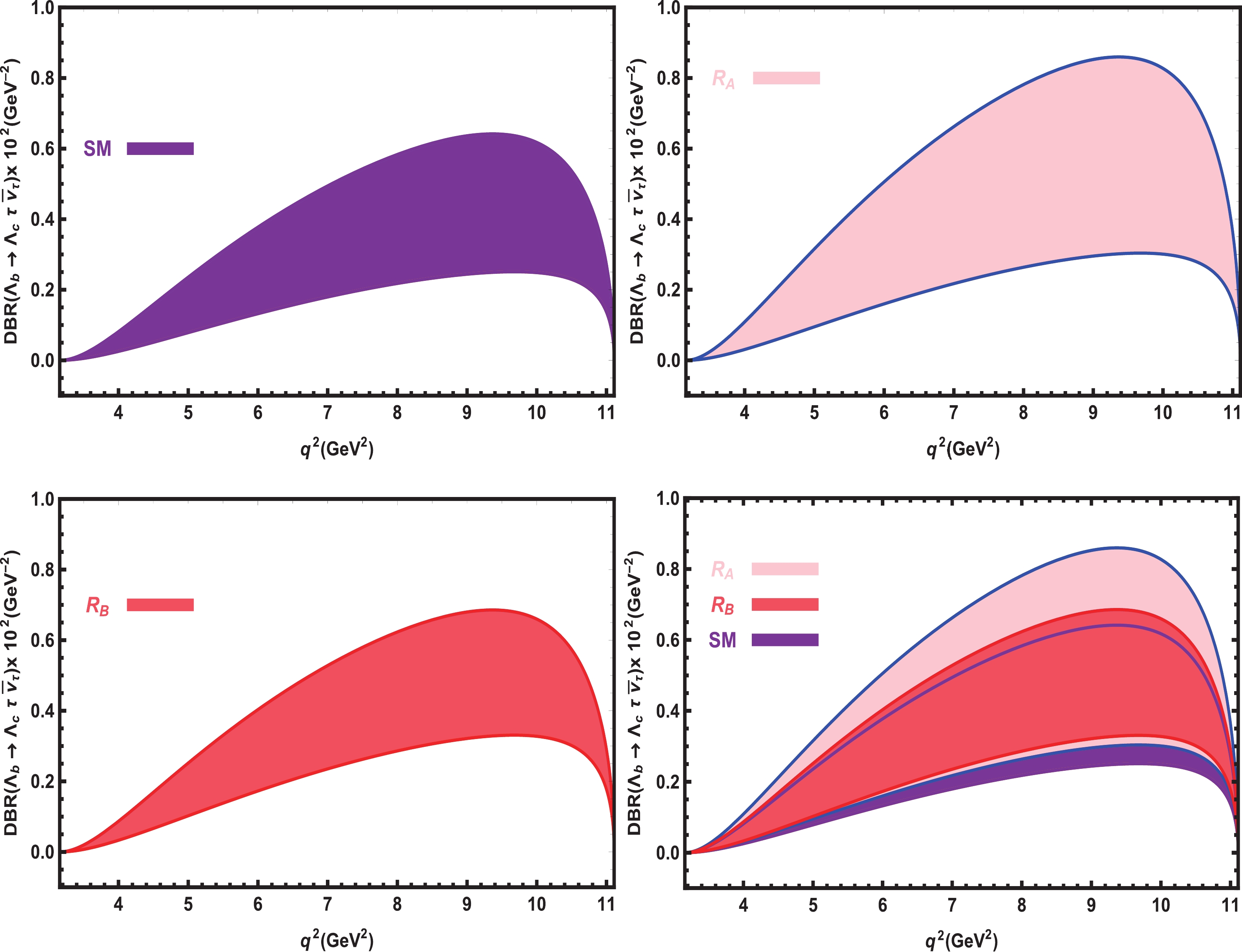 Figure2. (color online) The dependence of the


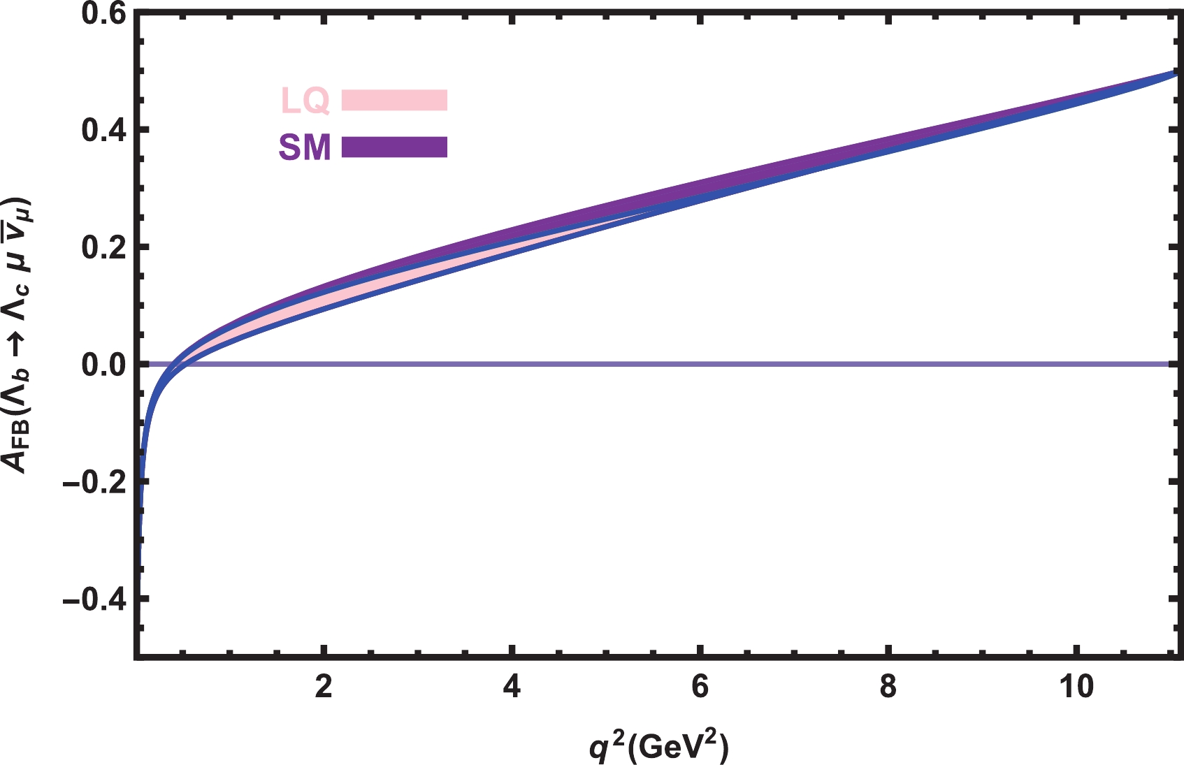 Figure3. (color online) The dependence of the
  Figure4. (color online) The dependence of the
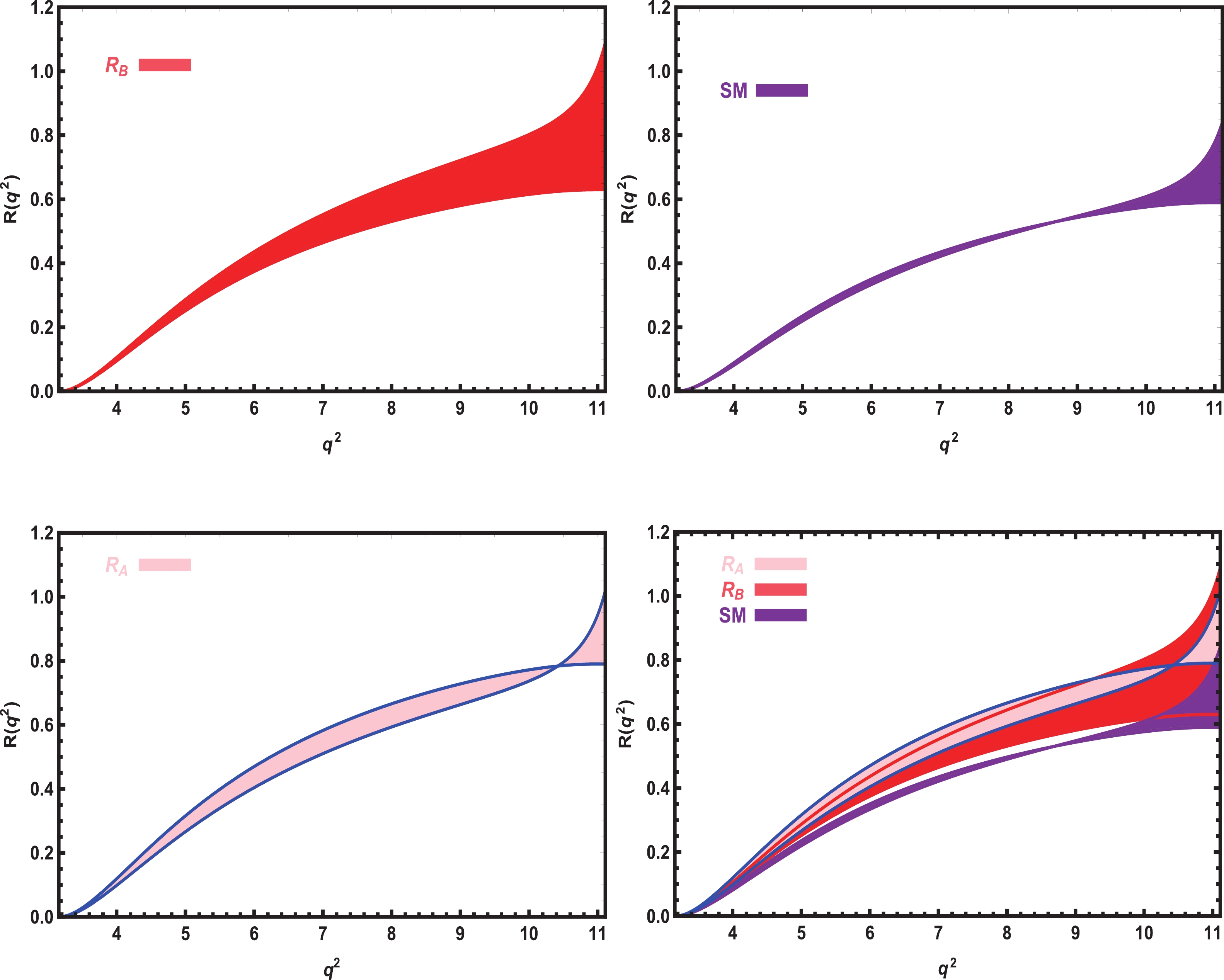 Figure5. (color online) The dependence of


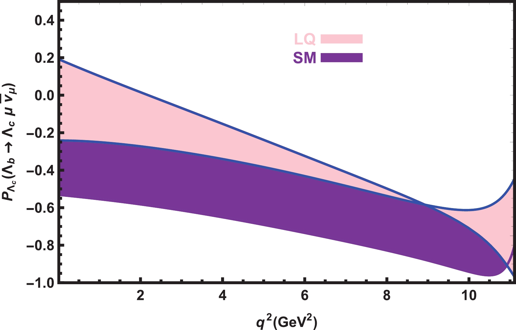 Figure6. (color online) The dependence of
  Figure7. (color online) The dependence of
 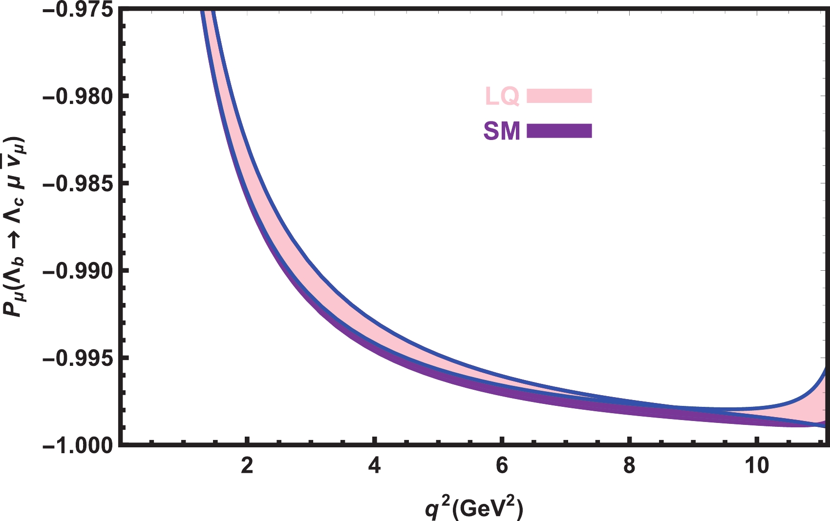 Figure8. (color online) The dependence of
 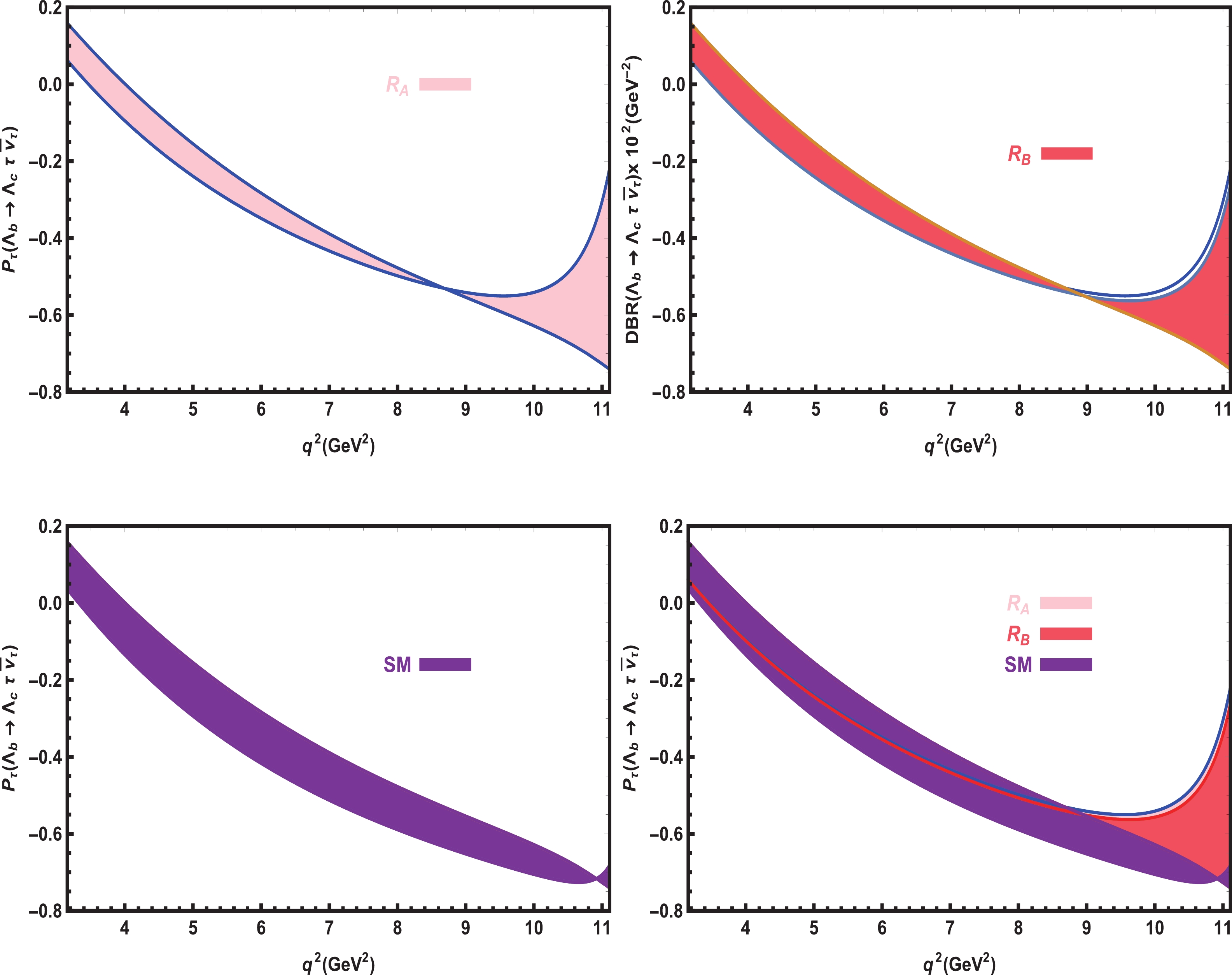 Figure9. (color online) The dependence of