Xu-Dong Sun
, Ben-Zhong Dai ^,
,

Corresponding author: Ben-Zhong Dai, bzhdai@ynu.edu.cn

School of Physics and Astronomy, Yunnan University, Kunming 650091, ChinaKey Laboratory of Astroparticle Physics, Yunnan Province, Kunming 650091, China
Received Date:2020-05-13
Accepted Date:2020-07-22
Available Online:2020-12-01
Abstract:Global symmetry can guarantee the stability of dark matter particles (DMps). However, the nonminimal coupling between dark matter (DM) and gravity can break the global symmetry of DMps, which in turn leads to their decay. Under the framework of nonminimal coupling between scalar singlet dark matter (ssDM) and gravity, it is worth exploring the extent to which the symmetry of ssDM is broken. It is suggested that the total number of decay products of ssDM cannot exceed current observational constraints. Along these lines, the data obtained with satellites such as Fermi-LAT and AMS-02 suggest that the scale of ssDM global symmetry breaking can be limited. Because the mass of many promising DM candidates is likely to be in the GeV-TeV range, we determine reasonable parameters for the ssDM lifetime within this range. We find that when the mass of ssDM is around the electroweak scale (246 GeV), the corresponding 3$\sigma$ lower limit of the lifetime of ssDM is $5.3\times10^{26}$ s. Our analysis of ssDM around the electroweak scale encompasses the most abundant decay channels of all mass ranges so that the analysis of the behavior of ssDM under the influence of gravity is more comprehensive.

HTML

--> --> -->

Observations of the rotation curves of galaxies, the Bullet Cluster, gravitationally lensed galaxy clusters, type Ia supernovae, baryonic acoustic oscillations, and anisotropies in the cosmic microwave background have all implied the existence of dark matter (DM) [1]. The standard model of particle physics successfully describes electromagnetism and weak and strong nuclear forces [2]; however, it does not currently accommodate the existence of dark matter particles (DMps). These statements suggest that physics beyond the standard model should be established [3, 4].
Among the various properties of DMps, we are concerned with their stability because if DMps are unstable, their decay products can be observed with satellites [5-7]. The stability of electrons is guaranteed by electric charge conservation, whereas the stability of neutrinos is guaranteed by Lorentz symmetry. Recent observations suggest that DM is stable and may be composed of particles. Typically, DMps are assumed to have global symmetry in Minkowski space-time, such as the hypothetical $ Z_2 $ symmetry [8, 9]. However, every particle is subject to gravitational interactions. In reality, there is no Minkowski space-time, and gravity does not minimally couple to DM. In the minimal coupling regime, matter distribution determines the distribution of gravitons, and gravitons and matter do not transform each other. However, if gravitons nonminimally couple to DM, then the global symmetry of DMps can be broken [10, 11]. Consequently, the stability of DMps is not preserved under the influence of gravity [12-15], implying that the decay of DMps occurs via nonminimal coupling with gravity.
O. Catà et al. [16, 17] have proposed models to describe how global symmetry breaking of scalar singlet dark matter (ssDM), inert doublet DM, and fermionic DM can be induced by nonminimal coupling with gravity. There have been other attempts to study the nonminimal coupling regime. For example, the Higgs field may have nonminimal coupling with gravity in Higgs inflation [18]. If the mass of a dark matter particle (DMp) is less than 270 MeV, then that particle could be acting concurrently as an inflaton [19]. There are also models of nonminimal coupling between DM and gravity where the global symmetry is not broken [20-22]. The nonminimal coupling between complex scalar DM and gravity has also been used to explain both the inflation and the electroweak phase transition [23, 24].
Many observations and experiments are needed to define the constraints on the global symmetry breaking of DMps. Currently, many types of experiments and observational methods are being used to search for DMps. Direct detection methods rely on monitoring the nucleon recoil induced by interactions with DMps distributed around the Earth [25]. Indirect detection methods search for photons, neutrinos, and/or cosmic rays produced by DMps using satellites and Earth-based instrumentation [26]. The Large Hadron Collider serves as a complementary experiment in the search for DM. Cosmological studies have defined constraints on DM. If nonminimal coupling with gravity breaks the global symmetry of DMps, then DM would be unstable. Consequently, DM would decay into observable particles such as cosmic rays [27], neutrinos [28], or cosmic gamma-rays [29]. Current observational techniques are still useful for defining the constraints on the stability of DMps, even though no conclusive particle signal has yet been attributed to DM [30].
O. Catà et al. [31] used chiral perturbation theory to determine the allowed parameter space of light ssDM particles (i.e., less massive than 1 GeV), in which the decay products have a sharp photon spectrum. These authors obtained the strongest constraints to date using Fermi-LAT gamma-ray observations. However, the mass of weakly interacting massive particles (WIMPs) and super WIMPs, based on the gauge hierarchy problem, and hidden DM, based on the gauge hierarchy problem and new flavor physics, is expected to be in the GeV–TeV range [32]. If the mass of a DMp is in the GeV–TeV range, more decay channels will be opened, and the decay properties of DMps will be quite diverse. Assuming that the lifetime of DMps is longer than the age of the universe and using observation data from neutrino telescopes, O. Catà et al. [16, 17] proposed rough restrictions on the nonminimal coupling coefficients between several widely studied DM candidates and the Ricci scalar in the GeV–TeV range.
In the case of DM decay, constraints obtained via indirect-detection methods play an important role. For example, satellites such as Fermi-LAT [33], Alpha Magnetic Spectrometer (AMS) [34], and DArk Matter Particle Explorer (DAMPE) [35] can obtain sensitive observations of high-energy photons and cosmic rays. In this work, we consider only the positron data obtained by AMS-02 [34] and photon data obtained by Fermi-LAT [33] to reveal conservative indirect restrictions of the GeV–TeV range because DAMPE is unable to distinguish positrons from electrons.
The action is constructed in the Jordan frame, according to the work of O. Catà et al. [17]. One can choose to calculate the specific decay channel in either the Jordan frame or Einstein frame when using Feynman diagrams. For example, J. Ren et al. [36] used the quantum field theory method to calculate Higgs inflation in Jordan and Einstein frames. They obtained the same result with both frames, indicating that the the Jordan and Einstein frames are equivalent in these scenarios. Then, in the Einstein frame, we calculate the spectra of photons and positrons arising from the decay of ssDM particles in the GeV–TeV range, where WIMPs, super WIMPs, and hidden DM mass are likely to be. Finally, we obtain constraints on the lifetime and the nonminimal coupling constant $ \xi $, which reflects the scale of the global symmetry breaking of ssDM particles, by comparing our theoretical spectra to observations made by Fermi-LAT and AMS-02.
The structure of this paper is as follows. In Section 2, we introduce the model and discuss the decay branch ratio of ssDM around the electroweak scale. In Section 3, we describe the calculation of the ssDM decay spectrum induced by global symmetry breaking. In Section 4, we explain the statistical methods used to compare the expected spectrum from decaying ssDM with the observed spectrum from Fermi-LAT and AMS-02. In Section 5, we provide the decay spectra of ssDM induced by global symmetry breaking and a reasonable parameter space for the lifetime of ssDM and the nonminimal coupling constant. The discussion and conclusions are presented in Section 6.

2

-->

2.1.The model

O. Catà et al. [16] considered that DM can nonminimally couple with the Ricci scalar, whose global symmetry is broken in curved space-time. In this paper, we focus on ssDM. In the Jordan Frame, the action $ {\cal{S}} $ of a system can be written as:

$ {\cal{S}} = \int {\rm d}^4x \sqrt{-g} \left[-\frac{R}{2\kappa^2}+{\cal{L}}_{\rm SM}+{\cal{L}}_{\rm DM} -\xi M \varphi R \right], $

(1)

where g is the determinant of metric tensor $ g_{\mu\nu} $.
The Einstein–Hilbert Lagrangian $ -R/2\kappa^2 $ describes the gravitational sector, where R is the Ricci scalar; $ \kappa = \sqrt{8\pi G} $ is the inverse (reduced) Planck mass, and G the Newtonian gravitational constant.
${\cal{L}}_{\rm SM}$ is the Standard Model Lagrangian that accurately describes the electromagnetism and the weak and strong nuclear forces at energies around the electroweak scale. It can be expressed as follows:

$ {\cal{L}}_{\rm SM} = {\cal{T}}_F+{\cal{T}}_f+{\cal{T}}_H+{\cal{L}}_Y-{\cal{V}}_H , $

(2)

where $ {\cal{V}}_H $ is the Higgs potential, $ {\cal{L}}_Y $ is the Yukawa interaction term, and $ {\cal{T}}_i $ are the kinetic terms of spin-one particles, fermions, and scalars.

$ {\cal{T}}_F = -\frac{1}{4}g^{\mu\nu}g^{\lambda\rho}F^a_{\mu\lambda}F^a_{\nu\rho}, $

(3)

$ {\cal{T}}_{f} = \frac{i}{2} \bar{f} \stackrel{\leftrightarrow}{\not\!{\nabla}} f, $

(4)

$ {\cal{T}}_H = g^{\mu\nu}(D_\mu \phi)^\dagger (D_\nu \phi). $

(5)

In these equations, the slashed derivative operator is defined as $\not\!{\nabla} = \gamma^a e^\mu_a \nabla_\mu$, where $ \nabla_\mu = D_\mu - \frac{i}{4} e^b_\nu (\partial_\mu e^{\nu c})\sigma_{bc} $, and $ e^{\nu c} $ is the vierbein. $ D_\mu $ represents the gauge covariant derivative, and $ \phi $ denotes the Higgs doublet.
In Eq. (1), ${\cal{L}}_{\rm DM} = {\cal{T}}_\varphi-V(\varphi,X)$ is the Lagrangian of ssDM, where $ \varphi $ represents ssDM. $ V(\varphi,X) $ is the DM potential. Because the DM potential contains interactions between ssDM and standard model particle X, it could be responsible for the correct DM relic abundance.
The research content of this paper comes from the last term of Eq. (1). Specifically, $ -\xi M \varphi R $ is the assumed non-minimal coupling operator between ssDM and gravity, where $ \xi $ is the coupling constant, and M is a parameter with dimension one so that $ \xi $ is dimensionless. For convenience, we set $ M = \kappa^{-1} $. This non-minimal coupling operator breaks the global $ {\mathbb{Z}}_2 $ symmetry of $ \varphi $, which causes ssDM to decay into standard model particles.
Using conformal transformation,

$ \tilde{g}_{\mu\nu} = \Omega^2 g_{\mu\nu}, $

(6)

where $ \Omega^2 = 1+2\xi M\kappa^2 \varphi $, and one can acquire action in the Einstein frame as

$ {\cal{S}} = \int {\rm d}^4x \sqrt{-\tilde{g}} \bigg[ -\frac{\tilde{R}}{2\kappa^2} +\frac{3}{\kappa^2} \frac{\Omega_{,\rho}\tilde{\Omega}^{,\rho}}{\Omega^2} +\tilde{{\cal{L}}}_{\rm SM}+\tilde{{\cal{L}}}_{\rm DM}\bigg], $

(7)

where

$ \tilde{{\cal{L}}}_{\rm SM} = \tilde{{\cal{T}}}_F+\Omega^{-3}\tilde{{\cal{T}}}_f+\Omega^{-2} \tilde{{\cal{T}}}_H+\Omega^{-4}({\cal{L}}_Y-{\cal{V}}_H), $

(8)

and $\tilde{{\cal{L}}}_{\rm DM} = \tilde{{\cal{T}}}_\varphi/\Omega^2-V(\varphi,X)/\Omega^{4}$. In these expressions, all tilded quantities are formed from $ \tilde{g}_{\mu\nu} $.
Eq. (8) indicates that DM $ \varphi $ could decay or annihilate into standard model particles through gravity portals. The Taylor expansion of Eq. (8) with respect to $ \xi $ shows that the dominant term is the decay term then becomes

$ \tilde{{\cal{L}}}_{\rm SM,\varphi} = -2\kappa\xi \varphi \bigg[\frac{3}{2}\tilde{{\cal{T}}}_f + \tilde{{\cal{T}}}_H +2({\cal{L}}_Y-{\cal{V}}_H)\bigg]. $

(9)

Using Eq. (9), O. Catà et al. [17] reported the Feynman rules for DM decay, as shown in Table 1.

terms from $ \tilde{{\cal{L}}}_{sm,\varphi} $ (2.7)	physical process	Feynman rules
$ \xi \kappa m_{f_i} \varphi \bar{f}_i f_i $	$ \varphi \rightarrow \bar{f}_i , f_i $	$ i\xi \kappa m_{f_i} $
$ - 3 \xi \kappa \varphi Y_\mu\bar{f}_i (\gamma^a e^\mu_a) ( a_{f_{ij}}-b_{f_{ij}}\gamma^5) f_j $	$ \varphi \rightarrow Y_\mu, \bar{f}_i, f_j $	$ - 3 i\xi \kappa (\gamma^a e^\mu_a) ( a_{f_{ij}}-b_{f_{ij}}\gamma^5) $
$ - \xi \kappa \varphi [ (\partial_\mu h)^2 - 2 m_h^2 h^2] $	$ \varphi \rightarrow h,h $	$ 2i\xi \kappa [p_{1\mu} p_2^\mu + 2 m_h^2 ] $
$ - \xi \kappa \varphi [2m_W^2 W^{\mu +} W_\mu^- + m_Z^2 Z^\mu Z_\mu ] $	$ \varphi \rightarrow Y_\mu , Y_\nu $	$ -2 i\xi \kappa m_{Y_\mu}^2 \tilde{g}^{\mu\nu} $
$ - 2 \xi \kappa \varphi \dfrac{h}{v} [2m_W^2 W^{\mu +} W_\mu^- + m_Z^2 Z^\mu Z_\mu ] $	$ \varphi \rightarrow h, Y_\mu , Y_\nu $	$ - 4 i\xi \kappa \dfrac{1}{v} m_{Y_\mu}^2 \tilde{g}^{\mu\nu} $
$ - \xi \kappa \varphi \dfrac{h^2}{v^2} [2m_W^2 W^{\mu +} W_\mu^- + m_Z^2 Z^\mu Z_\mu ] $	$ \varphi \rightarrow h,h,Y_\mu , Y_\nu $	$ - 4i\xi \kappa \dfrac{1}{v^2} m_{Y_\mu}^2 \tilde{g}^{\mu\nu} $
$ 4 \xi \kappa \varphi m_{f_i} \bar{f}_i f_i \frac{h}{v} $	$ \varphi \rightarrow h,\bar{f}_i , f_i $	$ 4 i\xi \kappa \dfrac{m_{f_i}}{v} $
$ 2 \xi \kappa \dfrac{m_h^2}{v} \varphi h^3 $	$ \varphi \rightarrow h,h,h $	$ 12 i\xi \kappa \dfrac{m_h^2}{v} $
$ \frac{1}{2} \xi \kappa \dfrac{m_h^2}{v^2} \varphi h^4 $	$ \varphi \rightarrow h,h,h,h $	$ 12i \xi \kappa \dfrac{m_h^2}{v^2} $
In the table, $f_i$ represents a fermion, and index i includes all fermion flavors. $Y_\mu$ represents a spin-one particle, and $a_{f_{ij}}$ and $b_{f_{ij}}$ can be obtained from the expansion of $\tilde{\cal{T}}_f$. $W^\mu$ represents the W boson; $Z^\mu$ represents the Z boson; h represents the Higgs boson; $v=246.2$ GeV is the Higgs vacuum expectation value; $m_{Y_\mu}$ represents the mass of the spin-one particle; $m_{f_i}$ represents the mass of the fermion; and $m_h$ represents the mass of the Higgs boson. The second column lists the decay channels. For example, $\varphi \rightarrow \bar{f}_i , f_i$ represents the channel through which DM $\varphi$ decays into a pair of fermions.

Table1.Feynman rules for DM decay.

2 -->

2.2.Branch ratio

The decay branch ratios of ssDM were drawn according to O. Catà et al. [16] and are shown in Fig. 1. O. Catà et al. also provided the asymptotic dependence of the corresponding partial width on the ssDM mass, using the limit of the massless final-state standard model particles, as shown in Table 2. This work focuses on the ssDM whose mass is around the electroweak scale.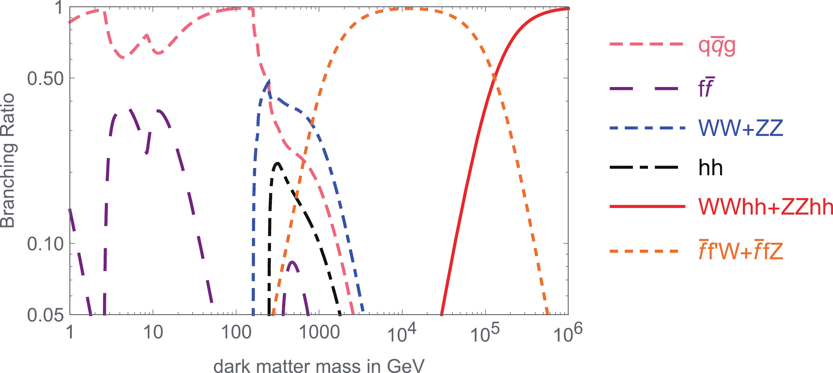
Figure1. (color online) Decay branch ratios of ssDM via non-minimal coupling with gravity.

Decay mode	Asymptotic scaling
$ \varphi\to hh, WW, ZZ $	$ m_\varphi^3 $
$ \varphi\to f\bar{f} $	$ m_\varphi m_f^2 $
$ \varphi\to hhh $	$ m_\varphi v^2 $
$ \varphi\to WWh,ZZh $	$ m_\varphi^5/ v^2 $
$ \varphi\to f\bar{f}h $	$ m_\varphi^3 m_f^2/ v^2 $
$ \varphi\to f'\bar{f}W,f\bar{f}Z $	$ m_\varphi^5/ v^2 $
$\varphi\to f\bar{f}\gamma,q\bar{q}g$	$ m_\varphi^3 $
$ \varphi\to hhhh $	$ m_\varphi^3 $
$ \varphi\to WWhh,ZZhh $	$ m_\varphi^7/v^4 $

Table2.Tree-level decay modes of ssDM [16].

Below the electroweak scale ($ m_\varphi < v $), the decay branch ratio is dominated by the $ \varphi\to q\bar{q}g $ channel. Although the asymptotic scaling of the $ \varphi\to f\bar{f}\gamma $ channel is also $ m_\varphi^3 $, it is suppressed by $ \alpha_{em}/\alpha_s $. Compared with the $ \varphi\to q\bar{q}g $ channel, $ \varphi\to f\bar{f}h $ channel is suppressed by $ m_f^2/v^2 $. The ratio of $ \varphi\to f\bar{f} $ channel to $ \varphi\to q\bar{q}g $ channel is $ m_f^2/m_\varphi^2 $. Therefore, when the mass of fermions is close to that of ssDM, the contribution of the $ \varphi\to f\bar{f} $ channel cannot be ignored. It is logical to recognize that in Fig. 1, the final-state particles of the $ \varphi\to f\bar{f} $ channel in the double-humped peak centered near 10 GeV are mainly tau leptons, charm quarks, and bottom quarks, and the final-state particles in the peak near 500 GeV are mainly top quarks.
Above the electroweak scale ($ 4\pi v \lesssim m_\varphi \lesssim 10^5\; {\rm{GeV}} $), the decay branch ratio is dominated by the $ \varphi\to f'\bar{f}W+f\bar{f}Z $ channel. Compared with the $ \varphi\to f'\bar{f}W+f\bar{f}Z $ channel, the $ \varphi\to q\bar{q}g $ channel is suppressed by the factor $ v^2/m_\varphi^2 $. Similarly, the $ \varphi\to hhh $ channel is suppressed by the factor $ v^4/m_\varphi^4 $. Although the asymptotic scaling of the $ \varphi\to WWh+ZZh $ channel is same as that of the $ \varphi\to f'\bar{f}W+f\bar{f}Z $ channel, it is suppressed by the smaller phase space.
Around the electroweak scale ($ m_\varphi\sim v $), many channels have an asymptotic scaling of $ m_\varphi^3 $, including $ \varphi\to WW+ZZ+hh+q\bar{q}g+\bar{f}f'W+f\bar{f}Z $. Because the mass of the top quark is also near the electroweak scale, the contribution from the $ \varphi\to f \bar{f} $ channel cannot be ignored. Therefore, the decay channels near the electroweak scale are the most abundant and worth a thorough analysis.
Only the channels shown in Fig. 1 were included in the following numerical calculations.

2

-->

3.1.Decay spectrum at production

Tanabashi et al. (Particle Data Group) [37] provided a detailed procedure to calculate decay rates and decay spectrum at production. These authors gave expressions for differential decay rates, e.g. Eq. (10), relativistically invariant three-body phase space, e.g. Eq. (11), and relativistically invariant four-body phase space, e.g. Eq. (14).
For convenience, we indicate the three product particles arising from three-body decay as particle 1, particle 2, and particle 3. The nomenclature used to indicate the rest frame of particle i and particle j is $ F_{ij} $.
The expression of the differential decay rate is

$ {\rm d}\Gamma = \frac{1}{2m_\varphi}|{\cal{M}}|^2 {\rm d}\Phi^{(n)}(m_\varphi;p_1,...,p_n), $

(10)

where $ \Gamma $ is the decay rate of $ \varphi $ in its rest frame; $ m_\varphi $ is mass of the DMp; $ {\cal{M}} $ is the invariant matrix element; $ \Phi^{(n)} $ is the n-body phase space; and $ p_i $ is the four momentum of terminal particle i. We also use the definitions $ p_{ij} = p_i+p_j $ and $ m_{ij}^2 = p_{ij}^2 $ so that the element of three body phase space ${\rm d}\Phi^{(3)}$ can be written as

$ {\rm d}\Phi^{(3)} = \frac{1}{2\pi} {\rm d}m_{12}^2 \frac{1}{16\pi^2} \frac{|\vec{p}_1^*|}{m_{12}}{\rm d}\Omega_{1}^* \frac{1}{16\pi^2} \frac{|\vec{p}_3|}{m_\varphi}{\rm d}\Omega_{3}, $

(11)

where ($ |\vec{p}_1^*|,\Omega_{1}^* $) is the three momentum of particle 1 in $ F_{12} $, and $ \Omega_3 $ is the angle of particle 3 in the rest frame of the decaying particle. The symbol $ * $ always denotes the quantity in $ F_{12} $.
The relationship between $ E_3 $ and $ m_{12} $ is

$ E_3 = \frac{m_{\varphi}^2+m_{3}^2-m_{12}^2}{2m_{\varphi}}, $

(12)

where $ m_3 $ and $ E_3 $ are the mass and energy of particle 3, respectively. The energy spectrum of particle 3 per decay in a channel with final state l can be calculated as follows:

$ \frac{{\rm d}{N}^l}{{\rm d}E_3} = \frac{\partial\Gamma^l}{\Gamma^l \partial E_3}. $

(13)

By using the Feynman rules listed in Table 1 and following Eqs. (10), (11), (12), and (13), we numerically calculated the decay rate $ \Gamma $ and energy spectrum ${\rm d}{N}^l/{\rm d}E_3$; ${\rm d}{N}^l/{\rm d}E_1$ and ${\rm d}{N}^l/{\rm d}E_2$ were calculated according to translatable symmetry , where $ E_1 $ is the energy of particle 1, $ E_2 $ is the energy of particle 2.
There are three channels for the four-body decay: $ \varphi\to W^+,W^-,h,h $; $ \varphi\to Z,Z,h,h $, and $ \varphi\to h,h,h,h $. We will consider $ \varphi\to W^+,W^-,h,h $ here to illustrate our method of calculation. The calculations of $ \Gamma $ and ${\rm d}{N}^l/{\rm d}E_1$ are demonstrated by regarding the $ W^+ $ boson as particle 1 and the $ W^- $ boson as particle 2; the remaining two Higgs bosons are particles 3 and 4. We continue to denote the rest frame of particles i and j as $ F_{ij} $, as noted earlier.
The element of four-body phase space ${\rm d}\Phi^{(4)}$ can be written as

$\begin{aligned}[b] {\rm d}\Phi^{(4)} =& \frac{1}{2\pi} {\rm d}m_{12}^2 \frac{1}{2\pi} {\rm d}m_{34}^2 \frac{1}{16\pi^2} \frac{|\vec{p}_1^*|}{m_{12}}{\rm d}\Omega_{1}^* \frac{1}{16\pi^2} \frac{|\vec{p}_3^{**}|}{m_{34}}\\&\times {\rm d}\Omega_{3}^{**} \frac{1}{16\pi^2} \frac{|\vec{p}_{12}|}{m_\varphi}{\rm d}\Omega_{12},\end{aligned} $

(14)

where ($ |\vec{p}_{12}|,\Omega_{12} $) is the three momentum of $ p_{12} $, and $ (\vec{p}_3^{**},\Omega_{3}^{**}) $ is the three momentum of particle 3 in $ F_{34} $. The symbol $ ** $ always denotes the quantity in $ F_{34} $. We numerically calculated $ \Gamma $ and $ \partial^2{N}^l/ (\partial m_{12}\partial m_{34}) $ using Eqs. (10) and (14), where $ \partial^2{N}^l/(\partial m_{12}\partial m_{34}) = \partial^2{\Gamma}^l/(\Gamma\partial m_{12}\partial m_{34}) $. We then applied Lorentz transformations to $ |\vec{p}_1^*| $ and $ E_1^* $. We find that the isotropic spectrum of particle 1 with momentum $ |\vec{p}_1^*| $ in $ F_{12} $ has a spectrum described by Eq. (15) in the rest frame of $ \varphi $:

$ g(E_1,m_{12}) = \frac{1}{2}\frac{1}{\gamma_{12}\beta_{12}|\vec{p}_1^*|} \Theta(E_1-E_-) \Theta(E_+-E_1), $

(15)

where $ \beta_{ij} $ is the velocity of $ F_{ij} $ relative to the decaying DMp; $ \gamma_{ij} = (1-\beta_{ij}^2)^{-1/2} $; $ E_\pm \equiv \gamma_{12}E_1^* \pm \gamma_{12}\beta_{12}|\vec{p}_1^*| $; and $ \Theta(x) $ is the Heaviside function.
The energy spectrum of particle 1 produced per decay in the channel with final state l can be described by

$ \frac{{\rm d}{N}^l}{{\rm d}E_1} = \int\int g(E_1,m_{12}) \frac{\partial^2{N}^l}{\partial m_{12}\partial m_{34}} {\rm d}m_{12}{\rm d}m_{34}. $

(16)

As before, ${\rm d}{N}^l/{\rm d}E_2$, ${\rm d}{N}^l/{\rm d}E_3$, and ${\rm d}{N}^l/{\rm d}E_4$ can also be calculated according to translatable symmetry, where $ E_2 $, $ E_3 $, and $ E_4 $ represent the energy of particles 2, 3, and 4, respectively.
Spectra have been obtained for many stable and unstable particles, such as the Higgs boson, Z boson, and neutrino. However, the spectra of final–state stable particles (i.e., photons and positrons) also need to be calculated for comparisons with observations. Cirelli et al. [38] used the PYTHIA codes to generate spectra of photons and positrons $ k(E,E_{\gamma,e^+}) $ induced by a primary state particle with energy E, where $ E_{\gamma,e^+} $ represents the energy of the photon or positron. The effects of QED and EW Bremsstrahlung were included when they used PYTHIA to generate $ k(E,E_{\gamma,e^+}) $, whereas the effects of inverse Compton processes and synchrotron radiation are not included [38]. The secondary photon or positron energy spectrum produced per decay in a channel with final state l represented by ${\rm d}{N}^l/{\rm d}E_{\gamma,e^+}$ was then numerically calculated as

$ \frac{{\rm d}{N}^l}{{\rm d}E_{\gamma,e^+}} = \sum\limits_s \int k(E_s,E_{\gamma,e^+}) \frac{{\rm d}{N}^l}{{\rm d}E_s} {\rm d}E_s , $

(17)

where s includes all final state particles in the channel with final state l. In the three-body decay case, s ranges from 1 to 3, whereas in the four-body decay case s ranges from 1 to 4.
2 -->

3.2.Fluxes after propagation

The spectra that can be detected by satellites are calculated via PPPC 4 DM ID [38]. In the following, we uniformly adopt the Navarro-Frenk-White (NFW) DM distribution model:

$ \rho(r) = \rho_s\frac{r_s}{r}\left(1+\frac{r}{r_s}\right)^{-2}, $

(18)

where $ \rho_s = 0.184\; {\rm{GeV}}/{\rm{cm}}^3 $; $ r_s = 24.42\; {\rm{kpc}} $; and $ \rho(r) $ is the energy density of DM at a distance of r from the galactic center.
The differential flux of positrons in space $ \vec{x} $ and time t is given by ${\rm d}\Phi_{e^+}/{\rm d}E_{e^+}(t,\vec{x},E_{e^+}) = v_{e^+}f/4\pi$, where $ v_{e^+} $ is the velocity of the positrons. The positron number density per unit energy f obeys the diffusion–loss equation [38, 39]:

$ \frac{\partial f}{\partial t}-\triangledown({\cal{K}}(E_{e^+},\vec{x})\triangledown f)-\frac{\partial}{\partial E_{e^+}}(b(E_{e^+},\vec{x})f) = Q(E_{e^+},\vec{x}) , $

(19)

where $ {\cal{K}}(E_{e^+},\vec{x}) $ is the diffusion coefficient function that describes the transport through turbulent magnetic fields. We adopt the customary parameterization of ${\cal{K}} = $ $ {\cal{K}}_0(E_{e^+}/{\rm{GeV}})^\delta = {\cal{K}}_0 \epsilon^\delta $ with the parameters ${\cal{K}}_0 = 0.0112 $ $ {\rm{kpc}}^2/{\rm{Myr}} $ and $ \delta = 0.70 $, which produce a median final result [38]. $ b(E_{e^+},\vec{x}) $ is the energy loss coefficient function that describes the energy lost from several processes, such as synchrotron radiation, inverse Compton scattering (ICS) of CMB photons, and infrared and optical galactic starlight. This coefficient is provided numerically by PPPC 4 DM ID [38] in the form of MATHEMATICA^? interpolating functions. Q is the source term that can be expressed as

$ Q = \frac{\rho(r)}{m_\varphi}\sum\limits_l \Gamma_l \frac{{\rm d}N_{e^+}^l}{{\rm d}E_{e^+}}. $

(20)

Eq. (19) is solved in a cylinder that sandwiches the galactic plane with height $ 2L $ and radius $ R = 20\; {\rm{kpc}} $. The distance between the solar system and the galactic center is 8.33 kpc. Conditions under which electrons/positrons can escape freely are adopted on the surface of the cylinder. The resulting differential flux of positrons in the solar system is

$ \begin{aligned}[b] \frac{{\rm d}\Phi_{e^+}}{{\rm d}E_{e^+}}(E_{e^+},r_\odot) =& \frac{v_{e^+}}{4\pi b(E_{e^+},r_\odot)} \frac{\rho_\odot}{m_\varphi} \sum\limits_l \Gamma_l \int_{E_{e^+}}^{m_\varphi/2} {\rm d}E_s \frac{{\rm d}N^l_{e^+}}{{\rm d}E_{e^+}} \\ &\times(E_s) I(E_{e^+},E_s,r_\odot), \end{aligned} ,$

(21)

where $ r_\odot $ is the distance between the solar system and the galactic center, and $ \rho_\odot $ is the DM density of the solar system. $ E_s $ is the positron energy at production (s stands for "source"). $ I(E_{e^+},E_s,r_\odot) $ is the generalized halo function, which is the Green function from a source with positron energy $ E_s $ to any energy $ E_{e^+} $, and it is also provided numerically by PPPC 4 DM ID [38] in the form of MATHEMATICA^? interpolating functions.
The calculation of gamma rays consists of three parts: the direct ("prompt") decay from the Milky Way halo, extragalactic gamma rays emitted by DM decay, and gamma rays from inverse Compton scattering (ICS). Synchrotron radiation is prevalent where the magnetic field and DM are very dense, near the galactic center. This work focuses on a high galactic latitude ($ |b|>20^\circ $) where the magnetic field is very weak; therefore, synchrotron radiation is not included in this work.
The differential flux of photons from the prompt decay of the Milky Way halo is calculated via

$ \frac{{\rm d}\Phi_\gamma}{{\rm d}E_\gamma {\rm d}\Omega} = \frac{r_\odot \rho_\odot}{4\pi m_\varphi} \bar{J} \sum\limits_l \Gamma_l \frac{{\rm d}N^l_\gamma}{{\rm d}E_\gamma} , $

(22)

where $\bar{J}(\triangle\Omega) = \int_{\triangle\Omega} J {\rm d}\Omega/\triangle\Omega$ is the averaged J factor of the region of interest; $J = \int_{\rm{l.o.s.}} \rho(r(s,\theta))/(r_\odot\rho_\odot) {\rm d}s$, $ r(s,\theta) = (r_\odot^2+s^2-2 r_\odot s {\rm{cos}}\theta)^{1/2} $ is the distance between the DM and the galactic center; and $ \theta $ is the angle between the direction of the line of sight (l.o.s.) and the line connecting the sun to the galactic center.
The extragalactic gamma rays received at a point with redshift z are calculated via [38]

$\begin{aligned}[b] \frac{{\rm d}\Phi_{{\rm{EG}}\gamma}}{{\rm d}E_\gamma}(E_\gamma,z) =& \frac{c}{E_\gamma}\int_{z}^{\infty} {\rm d}z' \frac{1}{H(z')(1+z')}\left(\frac{1+z}{1+z'}\right)^3 \\&\times\frac{1}{4 \pi} \frac{\bar{\rho}(z')}{m_\varphi}\sum\limits_l \Gamma_l \frac{{\rm d}N^l_\gamma}{{\rm d}E_\gamma'}(E_\gamma') {\rm e}^{-\tau(E_\gamma',z,z')}, \end{aligned}$

(23)

where $ H(z) = H_0\sqrt{\Omega_m (1+z)^3+(1-\Omega_m)} $ is the Hubble function; $ \bar{\rho}(z) = \bar{\rho}_0(1+z)^3 $ is the average cosmological DM density; and $ \bar{\rho}_0 \simeq 1.15\times 10^{-6}\; {\rm{GeV}}/{\rm{cm}}^3 $, $ E_\gamma' = E_\gamma(1+z') $, $ \tau(E_\gamma',z,z') $ are values for the optical depth provided numerically by PPPC 4 DM ID [38] in the form of MATHEMATICA^? interpolating functions. $ \tau(E_\gamma',z,z') $ describes the absorption of gamma rays in the intergalactic medium between the redshifts z and $ z' $. The presence of an ultraviolet (UV) background lowers the UV photon densities. There are three absorption models provided by PPPC 4 DM ID [38]: no ultraviolet (noUV), minimal ultraviolet (minUV), and maximal ultraviolet (maxUV). We calculated the Hubble function in the $ \Lambda $CDM cosmology with a pressure-less matter density of the universe $ \Omega_m = 0.27 $, dark energy density of the universe $ \Omega_\Lambda = 0.73 $, and a scale factor for Hubble expansion rate of $ 0.7 $.
Galactic electrons/positrons generated by ssDM could convert their energy into photons by inverse Compton scattering. The greater the mass of the ssDM, the higher the energy of the electrons/positrons generated by the ssDM, and the more important the effect. Inverse Compton gamma rays are calculated as follows:

$ \frac{{\rm d}\Phi_{{\rm{IC}}\gamma}}{{\rm d}E_\gamma {\rm d}\Omega} = \frac{1}{E_\gamma^2}\frac{r_\odot}{4\pi}\frac{\rho_\odot}{m_\varphi} \int_{m_e}^{m_\varphi/2} \!\!{\rm d}E_s \sum\limits_i \Gamma_i \frac{{\rm d}N_{e^+}^i}{{\rm d}E}(E_s) I_{{\rm{IC}}}(E_\gamma,E_s,b,l), $

(24)

where b and l are the galactic latitude and galactic longitude, respectively. $ I_{{\rm{IC}}}(E_\gamma,E_s,b,l) $ is a halo function for the IC radiation process, which is also provided numerically by PPPC 4 DM ID [38] in the form of MATHEMATICA^? interpolating functions.

2

-->

4.1.Statistical methods used to define constraints

The IGRB is measured using Fermi-LAT data [33]. We compared the $ \gamma $-ray flux produced by DM with the IGRB to define the constraints on the lifetime of ssDM. The region of interest includes high-latitude regions ($ |b|>20^\circ $), where b is the galactic latitude, because the analysis of the IGRB by Fermi-LAT is limited to these regions [33].
The cosmic positron flux is measured by the AMS on the International Space Station [34]. We also compared the positron flux produced by DM with the measured flux to define constraints on the lifetime of ssDM.
The comparison strategies used in this paper are as follows. Define $ \chi^2 $ as

$ \chi^2 = \sum\limits_i \frac{(\Phi^{\rm{th}}_i-\Phi^{\rm{obs}}_i)^2}{\delta_i^2} \Theta(\Phi^{\rm{th}}_i-\Phi^{\rm{obs}}_i), $

(25)

where $ \Phi^{\rm{th}}_i $ and $ \Phi^{\rm{obs}}_i $ denote the predicted and observed fluxes, respectively; $ \delta_i $ are the experimental errors, and $ \Theta(x) $ is the Heaviside function. This work requires $ \chi^2<9 $ to obtain an approximate estimate of the 3-$ \sigma $ constraint [40, 41], and only energy bins located above 1 GeV are used.
2 -->

4.2.Treatment of the background

Unresolved sources, such as non-blazar active galactic nuclei, the unresolved star-forming galaxies, BL Lacertae objects, flat-spectrum radio quasar blazars, and electromagnetic cascades generated through ultra-high energy cosmic-ray propagation, can contribute to the IGRB. When the IGRB is used to constrain the lifetime of DM, some studies consider the contribution of these sources to obtain the most stringent constraints [42]. Other studies do not consider the contribution of these sources to obtain conservative constraints [41]. In this study, we do not consider unresolved source contributions to the IGRB; therefore, the results we obtain are conservative.
The cosmic positron spectrum is believed to have a power-law background. We do not consider this contribution in the total predicted flux; therefore, the results obtained using the cosmic positron flux are also conservative.

The photon and positron flux values arising from DMp decay that would be detected by satellites were calculated based on the procedure outlined in Section 3.
Figure 2 shows the average photon flux values ($ |b|>20^\circ $) from the decaying DMps of the prompt emission, extragalactic, and inverse Compton scattering components and the total flux when the lifetime of ssDM is $ \tau = 5.3\times10^{26}\; s $, and the minUV model is adopted. The data in Fig. 2(a)-(c) show that when $ v<m_\varphi<1000\; {\rm{GeV}} $, prompt photon flux contributes the most to the total flux, and inverse Compton scattering contributes the least. When the mass of the ssDM is large enough (e.g., $ m_\varphi = 20\; {\rm{TeV}} $, as shown in Fig. 2(d)), the contribution of inverse Compton scattering to the low energy region of the photon spectrum is comparable with the contributions of prompt emission and extragalactic flux.
Figure2. (color online) Average photon flux values ($ |b|>20^\circ $) from decaying DMps of the prompt emission, extragalactic, and inverse Compton scattering components are shown by a dashed line, dotted line, and dot–dashed line, respectively, for $ \tau = 5.3\times10^{26}\; s $. The total flux of the three components is indicated by the black solid line. Fermi-LAT observations of the IGRB are indicated by blue points with error bars.

Figure 3 shows the average photon flux values ($ |b|>20^\circ $) from decaying DMps contributed by different channels when $ \tau = 5.3\times10^{26}\; s $ and the minUV model is adopted. The data in Fig. 3(a)–(c) show that when $ v<m_\varphi< $ 1000 GeV, the contributions of two-body decays are comparable with those of three-body channels. This result is consistent with Fig. 1 because when $ v<m_\varphi<1000\; {\rm{GeV}} $, the branching ratios of two-body decays are comparable with those of three-body channels. The $ \varphi\to h,h $ channel is the most characteristic among the channels, and its contribution to the photon flux increases slightly near the cut-off. When the mass of a DM particle is $ m_\varphi = 20\; {\rm{TeV}} $, the data in Fig. 3(d) indicate that the photons primarily originate from the $ \varphi\to \bar{f}f'W+\bar{f}fZ $ channel. This result is also consistent with Fig. 1 because when $ 4\pi v \lesssim m_\varphi \lesssim 10^5\; {\rm{GeV}} $, the branching ratio of the ssDM is dominated by the same channel.
Figure3. (color online) Average photon flux values ($ |b|>20^\circ $) from decaying DMps contributed by the indicated channels are shown for $ \tau = 5.3\times10^{26}\; s $. The total flux is indicated by the solid line. Fermi-LAT observations of the IGRB are indicated by blue points with error bars.

Figure 4 shows the absorption of UV photons in the presence of the UV background compared with no UV background when $ \tau = 5.3\times10^{26}\; s $. When $ v<m_\varphi< $ 1000 GeV, a comparison of the maximum of these discrepancies, as shown in Fig. 4(a)–(c), with the total flux, as shown in Fig. 2(a)–(c) or Fig. 3(a)–(c), yields $ (\Delta\Phi/\Phi)_{\rm{max}}\sim 10^{-2} $. When the mass of the ssDM is $ m_\varphi = 20\; {\rm{TeV}} $, a comparison of the maximum of the discrepancy, as shown in Fig. 4(d), with the total flux, as shown in Fig. 2(d) or Fig. 3(d), yields $ (\Delta\Phi/\Phi)_{\rm{max}}\sim 10^{-1} $. These results show that the absorption from the UV background becomes apparent when the mass of the DMps is large.
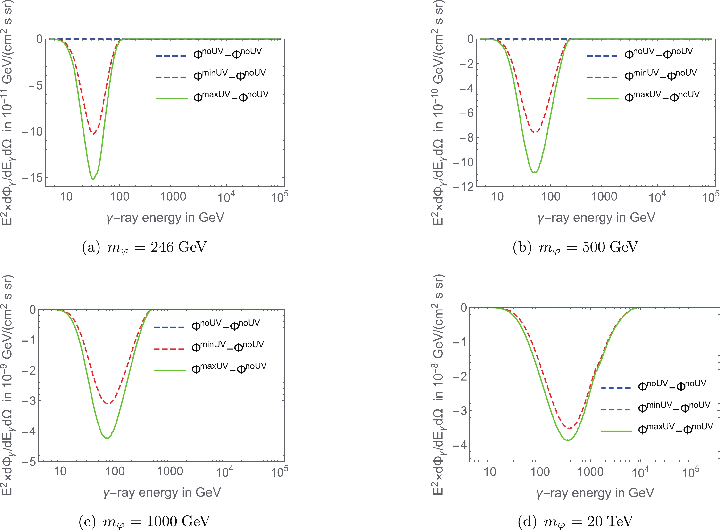Figure4. (color online) The presence of UV background lowers the UV photon density. The figure shows the absorption of UV photons compared with no UV background for$ \tau = 5.3\times10^{26}\; s $.

Figure 5 shows the positron flux from decaying DMps contributed by various channels when $ \tau = 10^{26}\; s $. Fig. 5(a) shows that when $ m_\varphi = v $, three–body decays tend to contribute positrons in the low energy region, whereas the $ \varphi\to WW+ZZ $ channel tends to contribute positrons in the high energy region. It could be inferred from Fig. 5(b) and 5(c) that when $ 500\; {\rm{GeV}}<m_\varphi<1000\; {\rm{GeV}} $, the contributions from two– and three–body decays are comparable. This result is consistent with Fig. 1 in that when $ 500\; {\rm{GeV}}<m_\varphi<1000\; {\rm{GeV}} $, the contribution of the branching ratio of two–body decays is comparable with that of the three-body channels. When the mass of the DMp is $ m_\varphi = 20\; {\rm{TeV}} $, the data in Fig. 5(d) show that the majority of positrons originate from the $ \varphi\to \bar{f}f'W+\bar{f}fZ $ channel. This result is consistent with Fig. 1 in that when $ 4\pi v \lesssim m_\varphi \lesssim 10^5\; {\rm{GeV}} $, the branching ratio of the ssDM is dominated by the same channel, as expected.
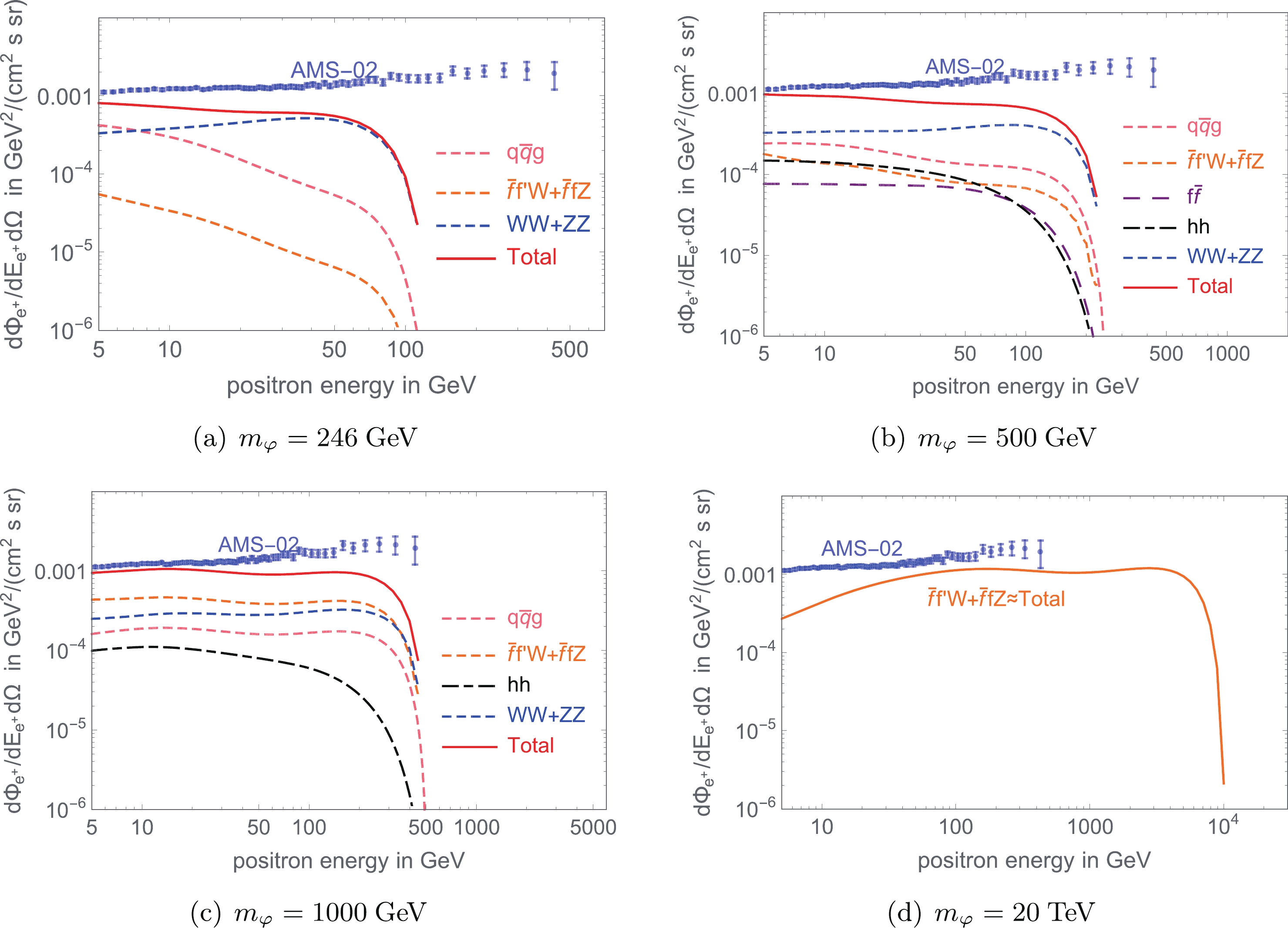Figure5. (color online) Predicted positron flux from decaying DMps contributed by the indicated channels are shown for $ \tau = 10^{26}\; s $. The total flux is indicated by the solid line. AMS-02 observations of positron flux are indicated by blue points with error bars [34].

The excluded two-dimensional parameter space ($ \tau,m_\varphi $), based on the procedure outlined in Section 4, is shown in Fig. 6, where the minUV model is adopted. The shaded area below the dashed line is the region of parameter space $ (\tau, m_\varphi) $, excluded by Fermi-LAT. The shaded area below the dotted line is the parameter space $ (\tau, m_\varphi) $ excluded by AMS-02. For comparison, a conservative excluded parameter space from observations of the cosmic neutrino flux [16, 17] is indicated by the shaded area below the dot–dashed line. We also plotted the line for $ \Lambda_{\rm{EW}} = 246 $ GeV, which represents the typical energy of the electroweak scale. If the mass of the DMp is around the electroweak scale, then the lifetime less than $ 5.3\times10^{26}\; s $ can be excluded. Because $ \xi $ reveals the effect of gravity on the global symmetry of ssDM, the excluded region of parameter space $ (\xi, m_\varphi) $ is shown in Fig. 7, where the minUV model is adopted.
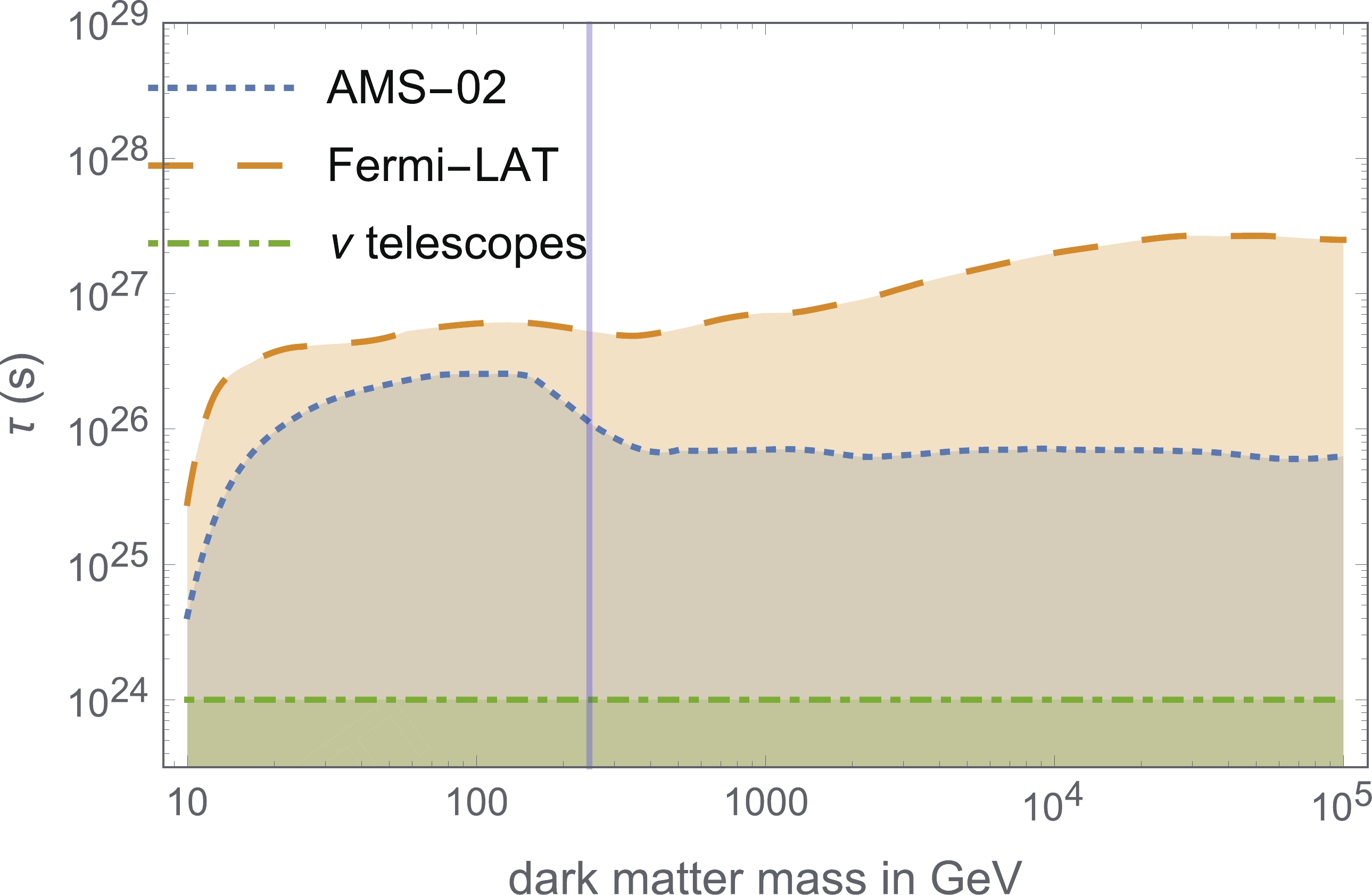Figure6. (color online) The $ \tau-m_\varphi $ plane. The shaded regions are excluded by observations of the IGRB by Fermi-LAT and the cosmic-ray positron spectrum obtained by AMS-02. For comparison, the conservative excluded parameter space from observations of the cosmic neutrino flux [16, 17] is indicated by the shaded area below the dot-dashed line.

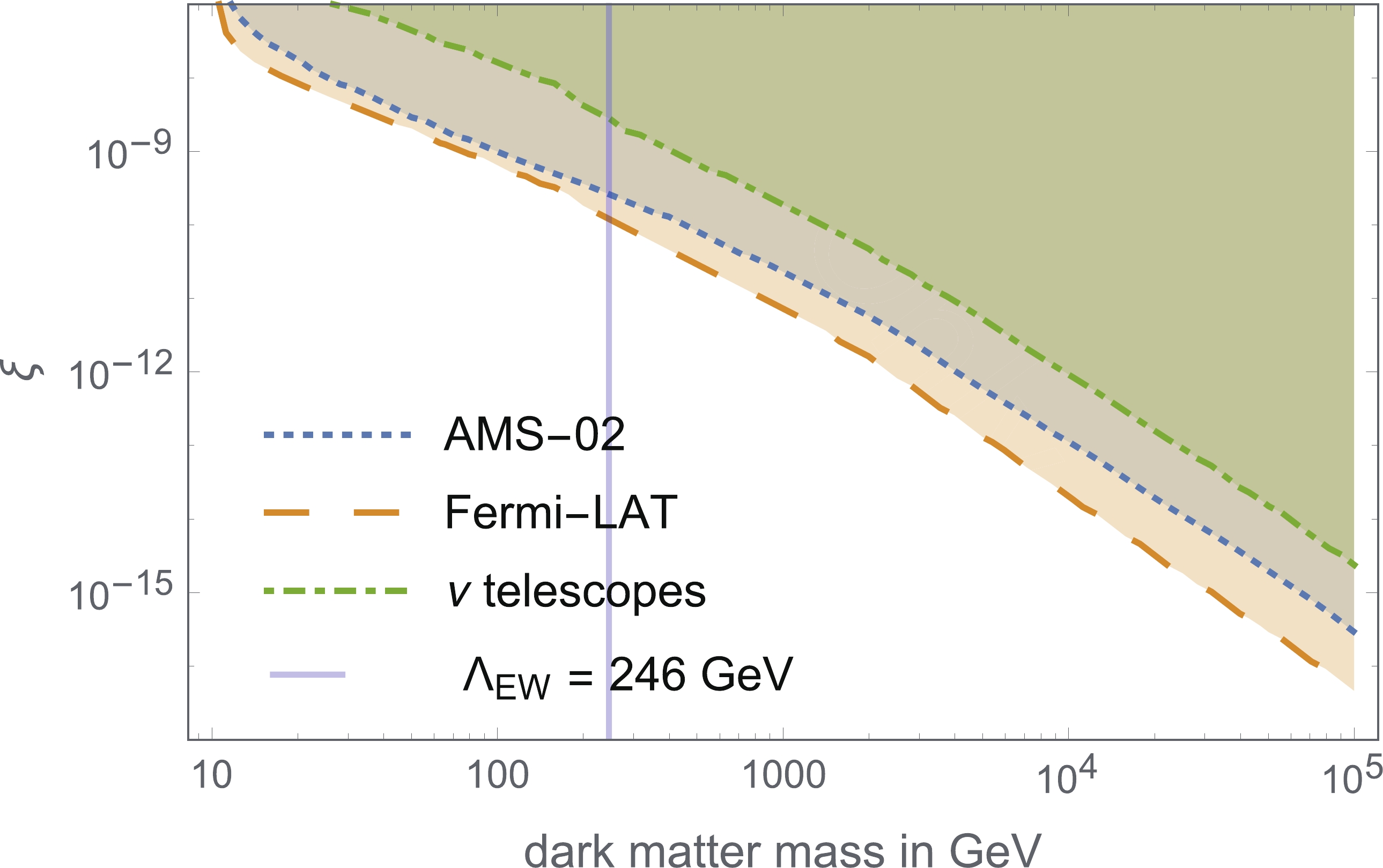Figure7. (color online) The $ \xi-m_\varphi $ plane. The shaded regions are excluded by observations of the IGRB by Fermi-LAT and the cosmic-ray positron spectrum obtained by AMS-02. For comparison, the conservative excluded parameter space from observations of the cosmic neutrino flux [16, 17] is indicated by the shaded area above the dot-dashed line.

Global symmetry can guarantee the stability of ssDM particles. However, nonminimal coupling between ssDM and gravity can break the global symmetry of the ssDM, leading to its decay.
In this study, we set constraints on the lifetime and the strength of symmetry breaking of ssDM particles using the most sensitive observations of photons and cosmic rays, respectively, made by Fermi-LAT and AMS-02. The data in Fig. 7 show that the non–minimal coupling constant between the Ricci scalar and ssDM is more constrained from indirect detection when the mass of ssDM is larger. This behavior is attributed to the fact that an ssDM particle with a larger mass has more decay channels and a larger phase space. This behavior also confirms the conclusion of O. Catà et al. that the exclusion of large regions of the parameter spaces in the GeV–TeV range requires additional stabilizing symmetry.
In contrast to previous work by [31], the masses of the ssDM particles considered in our study are around the GeV–TeV range. The decay channels around the GeV–TeV range are abundant, and the phase space is large. O. Catà et al. [31] showed that the lifetime of an ssDM candidate with a mass of approximately $ m_\varphi\gtrsim\; 1\; {\rm{MeV}} $ decaying through a gravity portal is constrained to $ \tau\gtrsim\; 10^{24}-10^{26}\; {\rm{s}} $. In this work, ssDM having a lifetime less than $ 5.3\times10^{26} $ is excluded at a 3–$ \sigma $ confidence level when the mass of the ssDM is around the electroweak scale (246 GeV). The mass region analyzed here contains abundant decay channels that the MeV scale does not have, so the analysis of the decay properties is comprehensive.
A new paper on this topic [43], being written in parallel with this work, points out that the fermionic fields should be conformally rescaled in the Einstein frame. In their study, all the vertices containing only one gauge boson disappear. Meanwhile, the decay rate of all other channels, including the $ \varphi\to\bar{f}_i,f_i $ channels, remains unchanged at tree level. Consequently, in the vicinity of the electroweak scale (i.e., $ v<m_\varphi<1000\; {\rm{GeV}} $), the constraints from the IGRB on the global symmetry of ssDM persist on the same order of magnitude as our study. However, in the region that deviates from the electroweak scale (i.e., $ m_\varphi<v $ and $ 10^3\; {\rm{GeV}}<m_\varphi<10^5\; {\rm{GeV}} $), the constraints from the IGRB on the global symmetry of ssDM are significantly weakened. Another related work in progress [44] describes a different framework for non-minimal coupling of DM with gravity. This framework differs from the one developed by O. Catà et al. in that the only allowed DM is scalar and couples only to the standard model Higgs boson. Therefore, any decay of DM is through the Higgs (either on-shell or off-shell).
Numerous theoretical and experimental works are in progress regarding the indirect detection of DM in the galactic region and beyond. On the theoretical side, S. Amoroso et al. [45] have produced spectra within PYTHIA 8.2 (which can be considered as updates to the PPPC 4 DM tables) following several improvements to the tuning of the PYTHIA 8 event generator and the perturbative machinery. Moreover, they estimated QCD uncertainties on particle spectra from showering and hadronization for the first time, which could prove useful for global fits. On the experimental side, the DAMPE detector was designed to run for at least three years, and the energies measured may reach 10 TeV [35]. The Large High Altitude Air Shower Observatory (LHAASO) can detect $ \gamma $-ray signals from DMps with masses in the PeV-EeV range decaying within a time scale of $ 3\times10^{29} $ s [46]. These missions will facilitate more detailed investigations of the impact of gravity on DM.