Liang-Liang Liu ^1,
, Xian-Wei Kang ^3,
, Zhen-Yang Wang ^2,
, Xin-Heng Guo ^3,,
,

Corresponding author: Xin-Heng Guo, xhguo@bnu.edu.cn

1.College of Physics and Information Engineering, Shanxi Normal University, Linfen 041004, China
2.Physics Department, Ningbo University, Zhejiang 315211, China
3.College of Nuclear Science and Technology, Beijing Normal University, Beijing 100875, China
Received Date:2020-03-25
Available Online:2020-08-01
Abstract:We study the rare decays $\Lambda_b \rightarrow \Lambda l^+ l^-~(l=e,\mu, \tau)$ in the Bethe-Salpeter equation approach. We find that the branching ratio is ${\rm Br}(\Lambda_b \rightarrow \Lambda \mu^+ \mu^-)\times 10^{6} = 1.051 \sim 1.098$ in our model. This result agrees with the experimental data well. In the same parametric region, we find that the branching ratio is ${\rm Br}(\Lambda_b \rightarrow \Lambda e^+ e^-(\tau^+ \tau^-) )\times 10^{6} = 0.252 \sim 0.392 ~(0.286 \sim 0.489)$.

HTML

--> --> -->

Recently, some interesting experimental results have been obtained in the studies of rare decays of b baryons induced by the $ b \rightarrow s $ transition [1-5]. The rare decay $ \Lambda_b \rightarrow \Lambda \mu^+ \mu^- $ was observed by the CDF [1] and LHCb [2] collaborations. The first observation of the baryonic flavor changing neutral current decay $ \Lambda_b \rightarrow \Lambda \mu^- \mu^+ $ by the CDF collaboration [1] had a signal yield of $ 24\pm5 $ events, corresponding to the absolute branching fraction ${\rm Br}(\Lambda_b \rightarrow \Lambda \mu^+ \mu^-) = (1.73\pm 0.42$ (stat) $ \pm $ (syst) $ )\times 10^{-6} $. Following previous measurements, the LHCb collaboration [2] reported the branching fraction of ${\rm Br}(\Lambda_b \rightarrow \Lambda \mu^+ \mu^-) = (0.96\pm 0.16$(stat)$ \pm 0.13 $(syst)$ \pm 0.21 $(norm)$ )\times 10^{-6} $ based on the $ 78\pm12 \; \Lambda_b \rightarrow \Lambda \mu^+ \mu^- $ events and updated experimental data ${\rm d} \Gamma(\Lambda_b \rightarrow \Lambda \mu^+ \mu^-)/{\rm d}q^2 = (1.18^{+0.09}_{-0.08}\pm 0.036 \pm 0.27)\times 10^{-7} {\rm GeV}^{-2}$ intergrating over $ 15<q^2<20 $ GeV$ ^2 $ [3]. The first observation of the radiative decay $ \Lambda_b \rightarrow \Lambda \gamma $ was reported in [4], and the branching fraction was measured as ${\rm Br}(\Lambda_b \rightarrow \gamma \Lambda) = (7.1\pm 1.56 \pm 0.6\pm 0.7)\times 10^{-6}$ based on the $ 65\pm13 \; \Lambda_b \rightarrow \Lambda\mu^+ \mu^- $ events with the significance of 5.6$ \sigma $. The analysis of the angular distribution of the decay $ \Lambda_b \rightarrow \Lambda \mu^+ \mu^- $ was reported in [5], and the first analysis of the differential fraction and the angular distribution of $ \Lambda_b \rightarrow \Lambda \mu^+ \mu^- $ was given in [3].
In the past several decades, significant theoretical efforts have been made to study the decays $ \Lambda_b \rightarrow \Lambda \gamma $ [6-13] and $ \Lambda_b \rightarrow \Lambda l^+ l^- $ [14-32]. In [6], the branching fraction ${\rm Br}(\Lambda_b \rightarrow \gamma \Lambda) = (1-4.5)\times 10^{-5}$ was reported based on the experimental data [31]. In [7], the branching fraction ${\rm Br}(\Lambda_b \rightarrow \gamma \Lambda) = 0.23\times 10^{-5}$ was given using the covariant oscillator quark model. Using the quantum chromodynamics (QCD) sum rules, in [12] it was reported that ${\rm Br}(\Lambda_b \rightarrow \gamma \Lambda) = (3.7\pm0.5) \times 10^{-5}$. Following this work, considering the long-distance effects, in [14] the decay branching ratios were $ 5.3\times 10^{-5} $ for $ \Lambda_b\rightarrow \Lambda l^+ l^- (l = e,\mu) $ and $ 1.1\times 10^{-5} $ for $ \Lambda_b\rightarrow \Lambda \tau^+ \tau^- $. Using the decay form factors (FFs) from [12], many studies addressed the rare decay $ \Lambda_b \rightarrow \Lambda l^+ l^- $ [15-21, 32]. In the relativistic quark model, the branching fractions were obtained in [10] as ${\rm Br}(\Lambda_b \rightarrow \Lambda l^+ l^-) \times 10^{-6} = 1.07\; (l = e), 1.05\; (l = \mu), 0.26\; (l = \tau)$.
However, in most of these works with the FFs of $ \Lambda_b \rightarrow \Lambda $ being based on light-cone QCD sum rules and assumed to have the same shape, the results for the branching ratios of $ \Lambda_b \rightarrow \Lambda l^+ l^- $ are different and do not agree with the existing experimental data. One important approach to search for new physics in b-physics is to analyze the rare B decay models that are induced by the flavor-changing neutral current (FCNC) transitions. The FCNC transitions are forbidden at the tree level in the standard model, and thus provide a good testing ground for new physics. To use $ \Lambda_b $ rare decays in search of new physics, the $ \Lambda_b \rightarrow \Lambda $ transition matrix must be determined more exactly.
In general, there could be other types of diquarks contributing to $ \Lambda_b $ and $ \Lambda $. However, considering that the b-quark is very heavy, the $ (ud) $ diquark has good spin and isospin quantum numbers, which are both zero in the heavy quark limit; hence, only the $ b(ud)_{00} $ composition is taken into account, which is dominant. Then, for the $ \Lambda_b \rightarrow \Lambda $ transition, only the $ s(ud)_{00} $ composition in $ \Lambda $ contributes.
This paper is organized as follows. In Section 2, we establish the BS equation for $ \Lambda_b $ and $ \Lambda $. In Section 3 we derive the FFs for $ \Lambda_b \rightarrow \Lambda $ in the BS equation approach. In Section 4 the numerical results for the FFs and the decay branching ratios of $ \Lambda_b \rightarrow \Lambda l^+ l^- $ are given. Finally, the summary and discussion are given in Section 5.

In our work, $ \Lambda_b $ can be described as a $ b(ud)_{00} $ system (the first and second subscripts correspond to the spin and the isospin of $ (ud) $, respectively). The BS wave function of the $ b(ud)_{0 0} $ system can be defined as follows [33-40]:

$ \chi(x_1,x_2,P) = \langle0|T\psi(x_1) \varphi(x_2)|P\rangle, $

(1)

where $ \psi(x_1) $ and $ \varphi(x_2) $ are the field operators of the b-quark and $ (ud)_{00} $ diquark, respectively, and P is the momentum of $ \Lambda_b $. We use $ M,\; m,\;{\rm{and}}\; m_D $ to represent the masses of the $ \Lambda_b $, the b-quark and the $ (ud) $ diquark, respectively. We define the BS wave function in the momentum space, as follows:

$ \chi(x_1,x_2,P) = {\rm e}^{{\rm i} P X}\int \frac{{\rm d}^4 p}{(2\pi)^4}{\rm e}^{{\rm i} p x} \chi_P(p), $

(2)

where $ X = \lambda_1 x_1+\lambda_2 x_2 $ is the coordinate of the center of mass, $ \lambda_1 = \dfrac{m }{m +m_D} $, $ \lambda_2 = \dfrac{m_D}{m +m_D} $, $ x = x_1-x_2 $, and p is the relative momentum of the quark and the diquark. As is show in Fig. 1 in the momentum space, the BS equation for $ \Lambda_b $ satisfies the homogeneous integral equation [33, 34, 36-40]
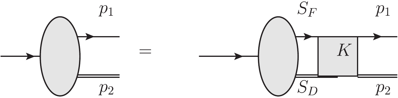Figure1. The BS equation for $ b(ud)_{00} $ system in the momentum space (K is the interaction kernel).

$ \begin{split} \chi_P(p) =& {\rm i} S_F(p_1)\int \frac{{\rm d}^4 q}{(2 \pi)^4} [ I\otimes I V_1(p,q)\\&+ \gamma_\mu \otimes \Gamma^\mu V_2(p,q) ]\chi_P(q)S_D(p_2), \end{split} $

(3)

where the quark momentum $ p_1 = \lambda_1 P+p $ and the diquark momentum $ p_2 = \lambda_2 P-p $, $ S_F(p_1) $ and $ S_D(p_2) $ are the propagators of the quark and the scalar diquark, respectively. $ V_1 $ and $ V_2 $ are the scalar confinement and one-gluon-exchange terms, respectively [41]. $\Gamma^\mu = (p_2+q_2)^\mu \dfrac{\alpha_{\rm seff}Q_0^2}{Q^2+Q^2_0}$ is introduced to describe the structure of the scalar diquark [6, 36, 42]. By analyzing the proton electromagnetic FFs, it was found that $ Q_0^2 = 3.2 $ GeV² can yield results that are consistent with the existing experimental data [6]. Motivated by the potential model, $ V_1 $ and $ V_2 $ have the following forms in the covariant instantaneous approximation ($ p_l = q_l $) [36, 37, 40, 43]:

$\begin{split} \tilde{V}_1(p_t-q_t) =& \frac{8 \pi \kappa}{[(p_t-q_t)^2+\mu^2]^2} - (2\pi)^2\delta^3(p_t-q_t)\\&\times\int \frac{{\rm d}^3k}{(2\pi)^3} \frac{8 \pi \kappa}{(k^2+\mu^2)^2}, \end{split}$

(4)

$ \tilde{V_2} (p_t-q_t) =- \frac{16 \pi }{3}\frac{\alpha_{\rm seff} }{(p_t-q_t)^2+\mu^2}, $

(5)

where $ q_t $ is the transverse projection of the relative momenta along the momentum P, defined as $ q_t^\mu = q^\mu -(v \cdot q) v^\mu $, $ q_l = \lambda_2 M -v \cdot q $ ($ v^\mu = P^\mu/M $). The second term of $ \tilde{V}_1 $ is introduced to avoid infrared divergence at the point $ p_t = q_t $, $ \mu $ is a small parameter to avoid the infrared divergence. The parameters $ \kappa $ and $\alpha_{\rm seff}$ are related to the scalar confinement and the one-gluon-exchange diagram, respectively.
In general, the $ b(ud)_{00} $ system needs two scalar functions to describe the BS wave function [33, 34, 38]

$ \chi_P(p) = (f_1(p_t^2)+{\not\!\!{p}}_t f_2(p_t^2))u(P), $

(6)

where $ f_i, (i = 1,2) $ are the Lorentz-scalar functions of $ p_t^2 $, $ u(P) $ is the spinor of $ \Lambda_b $, $ p_t $ is the transverse projection of the relative momenta along the momentum P, $ p_t^\mu = p^\mu-(v\cdot p) v^\mu $ and $ p_l = \lambda_2 M- v \cdot p $.
The quark and diquark propagators can be written as follows:

$ S_F(p_1) = {\rm i} {\not{v}} \bigg[ \frac{\Lambda_q^+ }{ M -p_l -\omega_q +{\rm i} \epsilon} +\frac{\Lambda_q ^-}{ M -p_l +\omega -{\rm i} \epsilon}\bigg], $

(7)

$ S_D(p_2) = \frac{\rm i}{2 \omega_D} \bigg[\frac{1}{ p_l-\omega_D+{\rm i} \epsilon} -\frac{1}{ p_l+ \omega_D-{\rm i}\epsilon}\bigg], $

(8)

where $ \omega_q = \sqrt{m^2-p_t^2}\; {\rm{and}}\; \omega_D = \sqrt{m_D^2-p_t^2} $. $ \Lambda^\pm_q = 1/2 \pm {\not\!{v}}({\not\!\!{p}}_t+m)/(2\omega_q) $ are the projection operators that satisfy the relations, $ \Lambda_q^\pm \Lambda_q^\pm = \Lambda^\pm_q,\; \Lambda^\pm_q \Lambda^\mp_q = 0 $. On the order of $ \dfrac{1}{m} $ [36], the quark propagator can be written as

$ S_F(p_1) = {\rm i} \frac{ 1+ {\not\!{v}} }{ 2 (E_0+m_D -p_l+ {\rm i} \epsilon) }, $

(9)

where $ E_0 = M-m-m_D $ is the binding energy. In general, $ E_0 $ is approximately $ -0.14 \pm 0.05 $ GeV [38]; then, the diquark mass is approximately $ 0.75 $ GeV, which is in a good agreement with [44]. Then, we obtain that $ \kappa $ is approximately $ 0.05\pm0.01 $ GeV$ ^3 $ for $ \Lambda_b $ [39]. Defining $\tilde{f}_{1(2)} = \int \dfrac{{\rm d} p_l}{2 \pi}f_{1(2)}$, and using the covariant instantaneous approximation, $ p_l = q_l $, the scalar BS wave functions satisfy the coupled integral equation

$ \tilde{f}_1(p_t) = \int \frac{{\rm d}^3q_t}{(2\pi)^3} M_{11}(p_t,q_t) \tilde{f}_1(q_t)+ M_{12}(p_t,q_t) \tilde{f}_2(q_t) , $

(10)

$ \tilde{f}_2(p_t) = \int \frac{{\rm d}^3q_t}{(2\pi)^3} M_{21}(p_t,q_t) \tilde{f}_1(q_t) + M_{22}(p_t,q_t) \tilde{f}_2(q_t), $

(11)

where

$ \begin{split}M_{11}(p_t,q_t) =& \frac{(\omega_q +m ) (\tilde{V}_1+ 2 \omega_D \tilde{V}_2)- p _t \cdot ( p _t+ q _t) \tilde{V}_2}{4 \omega_D \omega_q(-M + \omega_D+ \omega_q)} \\&- \frac{(\omega_q -m )(\tilde{V}_1- 2\omega_D \tilde{V}_2)+ p _t\cdot( p _t+ q _t) \tilde{V}_2}{4 \omega_D \omega_c(M + \omega_D+ \omega_q)}, \end{split}$

(12)

$ \begin{split}M_{12}(p_t,q_t) =& \frac{- (\omega_q+m ) ( q _t + p _t)\cdot q_t\tilde{V}_2 + p _t\cdot q_t(\tilde{V}_1- 2 \omega_D \tilde{V}_2)}{4 \omega_D \omega_c(-M + \omega_D+ \omega_c)} \\& -\frac{(m - \omega_q ) ( q _t + p _t)\cdot q _t \tilde{V}_2 - p _t\cdot q _t (\tilde{V}_1+ 2\omega_D \tilde{V}_2)}{4 \omega_D \omega_q(M + \omega_D+ \omega_q)}, \end{split} $

(13)

$ \begin{split} M_{21}(p_t,q_t) =& \frac{(\tilde{V}_1+ 2 \omega_D \tilde{V}_2)-( -\omega_q+m) \dfrac{( p _t+ q _t) \cdot p _t }{ p^2_t }\tilde{V}_2}{4 \omega_D \omega_q(-M + \omega_D+ \omega_q)} \\&- \frac{- (\tilde{V}_1- 2\omega_D \tilde{V}_2)+(\omega_q + m )\dfrac{ ( p _t+ q _t)\cdot p _t }{ p^2_t } \tilde{V}_2 }{4 \omega_D \omega_q(M + \omega_D+ \omega_q)}, \end{split}$

(14)

$ \begin{split} M_{22}(p_t,q_t) =& \frac{(m -\omega_q)( \tilde{V}_1+ 2 \omega_D \tilde{V}_2) ) \dfrac{ p_t \cdot q_t}{ p^2_t } - ( q^2_t+ p_t \cdot q_t) \tilde{V}_2}{4 \omega_D \omega_q(-M + \omega_D+ \omega_q)} \\& -\frac{ (m +\omega_q) (-\tilde{V}_1- 2 \omega_D \tilde{V}_2) \dfrac{p_t \cdot q_t}{p^2_t} + ( q^2_t+ p_t \cdot q_t)\tilde{V}_2}{4 \omega_D \omega_q(M + \omega_D+ \omega_q)}. \end{split} $

(15)

The discussion about the BSE of $ \Lambda $ is similar. In Eq. (3), when $ \frac{1}{m_b}\rightarrow 0 $, $ \gamma_\mu $ can be replaced by $ v_\mu $, and we find that the BSE for $ \Lambda_b $ has the following form [36]

$ \begin{split} \phi(p) =& -\frac{\rm i}{(E_0+m_D-p_l+{\rm i} \epsilon)( p_l ^2-\omega^2_D)}\\&\times\int \frac{{\rm d}^4 q }{(2\pi)^4}(\tilde{V}_1+2 p_l \tilde{V}_2)\phi(q). \end{split} $

(16)

Then, considering that ${\not\!{v}} S_F(p_1) = S_F(p_1)$, we find that ${\not\!{v}} \chi_P(p) = \chi_P(p)$. Therefore, the BS wave function of $ \Lambda_b $ can be written as $ \chi_P (v) = \phi (p)u_{\Lambda_b}(v,s) $ where $ \phi(p) $ is a scalar function.
In general, the BS wave function can be normalized under the condition of the covariant instantaneous approximation [43]:

$ {\rm i} \delta^{i_1 i_2}_{j_1 j_2} \int \frac{{\rm d}^4 q {\rm d}^4 p}{(2\pi)^8}\bar{\chi}_P(p,s)\left[\frac{\partial}{\partial P_0}I_p(p,q)^{i_1 i_2 j_2 j_1}\right]\chi_P(q,s^\prime) = \delta_{s s^\prime}, $

(17)

where $ i_{1(2)} $ and $ j_{1(2)} $ represent the color indices of the quark and the diquark, respectively, $ s^{(\prime)} $ is the spin index of the baryon $ \Lambda_b $, $ I_p(p,q)^{i_1 i_2 j_2 j_1} $ is the inverse of the four-point propagator, written as follows:

$ I_p(p,q)^{i_1 i_2 j_2 j_1} = \delta^{i_1 j_1}\delta^{i_2 j_2} (2 \pi)^4 \delta^4(p-q)S^{ -1 }_F(p_1)S^{ -1 }_D(p_2).\\ $

(18)

In this section, we derive the matrix element of $ \Lambda_b\rightarrow\Lambda l^+ l^- $ in the BS equation approach. On the quark level, $ \Lambda_b\rightarrow\Lambda l^+l^- $ is described by the $ b\rightarrow s l^+l^- $ transition. The effective Hamiltonian describing this process can be given as the following [45]

$ \begin{split} {\cal H} =& \frac{G_F\alpha}{\sqrt{2}\pi}V_{tb}V^*_{ts}\bigg\{ \bar{s}\bigg[C^{\rm eff}_9 \gamma_{\mu}P_L -{\rm i} C^{\rm eff}_{7}\frac{2 m_b\sigma_{\mu\nu} q^{\mu}}{q^2}P_R \bigg]b(\bar{l}\gamma_{\mu}l)\\&+C_{10}(\bar{s}\gamma_{\mu}P_L b) (\bar{l}\gamma^{\mu}\gamma_5l) \bigg\}, \\[-18pt] \end{split}$

(19)

where $ G_F $ and $ \alpha $ are the Fermi coupling constant and the electromagnetic coupling constant, respectively, $ P_{R,L} = (1\pm \gamma_5)/2, $ q is the total momentum of the lepton pair, and $ C_i\; (i = 7,\; 9,\; 10) $ are the Wilson coefficients. The amplitude of the decay $ \Lambda_b \rightarrow \Lambda l^+ l^- $ is obtained by calculating the matrix element of the effective Hamiltonian for the $ b \rightarrow s l^+ l^- $ transition between the initial and final states, $ \langle \Lambda | {\cal H}|\Lambda_b\rangle $. The matrix element can be parameterized in terms of the FFs, as follows:

$ \begin{split} \langle\Lambda(P',s')\uparrowvert \bar{s}\gamma_{\mu}b\uparrowvert\Lambda_b(P,s)\rangle =& \bar{u}_{\Lambda}(P',s')(g_1\gamma^\mu+ ig_2\sigma_{\mu\nu}q^{\nu}+g_3q_\mu)u_{\Lambda_b}(P,s),\\ \langle\Lambda(P',s')\uparrowvert \bar{s}\gamma_{\mu}\gamma_{5}b\uparrowvert\Lambda_b(P,s)\rangle =& \bar{u}_{\Lambda}(P',s')(t_1\gamma^\mu+it_2\sigma_{\mu\nu}q^{\nu}+t_3q^\mu)\gamma_5u_{\Lambda_b}(P,s),\\ \langle\Lambda(P',s')\uparrowvert \bar{s}i\sigma^{\mu\nu}q^{\nu}b\uparrowvert\Lambda_b(P,s)\rangle =& \bar{u}_{\Lambda}(P',s')(s_1\gamma^\mu+is_2\sigma_{\mu\nu}q^{\nu}+s_3q^\mu)u_{\Lambda_b}(P,s),\\ \langle\Lambda(P',s')\uparrowvert \bar{s}i\sigma^{\mu\nu}\gamma_5q^{\nu}b\uparrowvert\Lambda_b(P,s)\rangle =& \bar{u}_{\Lambda}(P',s')(d_1\gamma^\mu+id_2\sigma_{\mu\nu}q^{\nu}+d_3q^\mu)\gamma_5u_{\Lambda_b}(P,s), \end{split} $

(20)

where $ q = P-P' $ is the momentum transfer, and $ g_i $, $ t_i $, $ s_i $, $ d_i $ ($ i = 1,2 $ and 3) are the various form factors, which are the Lorentz scalar functions of $ q^2 $. Considering the spin symmetry on the b quark in the limit $ m_b\rightarrow \infty $, the matrix elements in Eq. (20) can be rewritten as

$ \begin{split} \langle\Lambda(P',s')\uparrowvert \bar{s}\Gamma_{\mu} b\uparrowvert \Lambda_b(v,s)\rangle =& \bar{u}_{\Lambda}(P',s')(F_{1}(\omega)\\&+F_2(\omega){\not\!\!{v}})\Gamma^{\mu}u_{\Lambda_b}(v,s), \end{split}$

(21)

where $ \Gamma_{\mu} $ represents $ \gamma_{\mu} $, $ \gamma_{\mu}\gamma_5 $, $ i\sigma_{\mu\nu}q^{\nu} $, and $ i\sigma_{\mu\nu}\gamma_5q^{\nu} $. $ F_i $ ($ i = 1, 2 $) can be expressed as functions solely of $ \omega = \dfrac{ m^2_{\Lambda_b} + m^2_{\Lambda} -q^2 }{ 2 m_{\Lambda_b} m_{\Lambda} } = v\cdot P'/m_{\Lambda} $, which is the energy of the $ \Lambda $ baryon in the $ \Lambda_b $ rest frame.
In the pole formulae for the extrapolation to $ q^2 = 0 $ in the decay $ \Lambda_b \rightarrow \Lambda \gamma $ one has $ F_1(0) = 0.45 $ (monopole) and $ F_1(0) = 0.22 $ (dipole) [6], while in [6] CLEO data from [31] were combined, to obtain $F_1(q^2_{\max}) = 1.21$ , ignoring the mass of $ \Lambda $ baryon. Lattice QCD (LQCD) gives $F_1(q^2_{\max} )\approx 1.25$ in the leading order in the heavy quark effective theory [46]. In [47] it was assumed that $ F_2 = 0 $. The QCD sum rules analysis yielded $ F_1 = 0.50\pm0.03 $ and $ F_2 = -0.1\pm0.03 $ at the point $ E_0 = (m_{\Lambda_b}^2+m_\Lambda^2)/ (2 m_{ \Lambda_b}) = 2.93 $ GeV. Therefore, we expect $F_1(q^2_{\max}) < 1.5$, considering the correction of $\Lambda_{\rm QCD}/m_b$. The ratio $ R = F_2/F_1 = -0.35\pm0.04 $ (stat) $ \pm0.04 $ (syst) has been previously measured by the CLEO collaboration using experimental data for the semileptonic decay $ \Lambda_c \rightarrow \Lambda e^+ \nu_e $ with the invariant mass in the range from $ m_\Lambda $ to $ m_{\Lambda_c} $, assuming the same shape for $ F_1 $ and $ F_2 $ and ignoring the $\Lambda_{\rm QCD}/m_c$ corrections [48]. In [12] $ R = -0.42\; (-0.83) $ was given at $q^2 = q^2_{\max}(q^2 = 0)$, and in [32] $ R(0) \equiv -0.17 $ and $R(q_{\max}^2 = m^2_{\Lambda_c}) = -0.44$ were obtained. However, according to the pQCD scaling law, the FFs should have different shapes for large $ q^2 $ [42, 49, 50]; therefore, we expect $ R(q^2)\propto -1/q^2 $, which agrees with the results in [13]. Using experimental data [48], we have estimated the value of $R(q^2_{\max} = (m_{\Lambda_b}-m_\Lambda)^2)$ and found it to be ranging from $ -1.12 $ to $ -0.7 $ approximately. Considering the results in [12], we let $R(q^2_{\max})$ vary from $ -0.83 $ to $ -0.7 $.
Comparing Eq. (20) with Eq. (21), we obtain the following relations:

$ \begin{split}& g_1\; = \; t_1\; = \; s_2\; = \; d_2\; = \; \bigg(F_1+\sqrt{r}F_2\bigg),\\ & g_2\; = \; t_2\; = g_3\; = \; t_3\; = \; \frac{1}{m_{\Lambda_{b}}}F_2, \\ & s_3\; = \; F_2 (\sqrt{r}-1),\; d_3\; = \; F_2(\sqrt{r}+1), \\ & s_1 \; = \; d_1\; = \; F_2 m_{\Lambda_b} (1+r-2\sqrt{r}\omega),\end{split} $

(22)

where $ r = m_{\Lambda}^2/m_{\Lambda_b}^2 $. The transition matrix for $ \Lambda_b\rightarrow \Lambda $ can be expressed in terms of the BS wave function of $ \Lambda_b $ and $ \Lambda $

$ \langle\Lambda(P',s')|\bar{s}\Gamma_{\mu}b|\Lambda_b(P,s)\rangle = \int\frac{{\rm d}^4p}{(2\pi)^4} \bar{\chi}_{P'}^{\Lambda}(p')\Gamma_{\mu}\chi_P^{\Lambda_b}(p)S^{-1}_D(p_2). $

(23)

Define

$ \begin{split} &\int \frac{{\rm d}^4p}{(2 \pi)^4} f_1(p^\prime) \phi(p) S^{-1}_D(p_2) = k_1(\omega), \\ & \int \frac{{\rm d}^4p}{(2 \pi)^4} f_2(p^\prime)p_{t\mu}^\prime \phi(p) S^{-1}_D(p_2) = k_2(\omega) v_{\mu} + k_3(\omega) v^\prime_{\mu}, \end{split}$

(24)

where $ v^\prime = P^\prime/m_\Lambda $. Then, we find the following relations with $ \omega \neq 1 $

$ \begin{split} k_3 & = - \omega k_2, \\ k_2 & = \frac{1}{1-\omega^2} \int \frac{{\rm d}^4 p}{(2\pi)^4} f_2(p^\prime) p^\prime_t \cdot v \phi(p) S^{-1}_D, \end{split}$

(25)

and

$ \begin{split}&F_1 = k_1- \omega k_2 , \\ & F_2 = k_2.\end{split} $

(26)

The differential decay rate is obtained as follows:

$ \begin{split} {\cal M}(\Lambda_b\rightarrow \Lambda l^{+} l^{-}) =& \frac{G_F}{ \sqrt{2}\pi}\times \lambda_t\big[\bar{l}\gamma_{\mu}l\{\bar{u}_{\Lambda}[\gamma_{\mu}(A_1P_R +B_1P_L)\\&+i\sigma^{\mu\nu}p_{\nu}(A_2 P_R +B_2P_L)]u_{\Lambda_b}\} \\ &+\bar{l}\gamma_{\mu}\gamma_5l\{\bar{u}_{\Lambda}[\gamma^{\mu}(D_1P_R +E_1P_L)\\&+i\sigma^{\mu\nu}p_{\nu}(D_2P_R+E_2P_L)\\ &+p^{\mu}(D_3P_R+E_3P_L)]u_{\Lambda_b}\}\big], \end{split} $

(27)

where the parameters $ A_i $, $ B_i $ and $ D_j $, $ E_j $ ($ i = 1,2 $ and $ j = 1,2,3 $) are defined as

$ \begin{split} &A_i = \frac{1}{2}\bigg\{C^{\rm eff}_{9}(g_i-t_i)-\frac{2C^{\rm eff}_7 m_b}{p^2}(d_i +s_i )\bigg\},\\ & B_i = \frac{1}{2}\bigg\{C^{\rm eff}_{9}(g_i+t_i) - \frac{2C^{\rm eff}_7m_b}{p^2}(d_i -s_i )\bigg\}, \\ & D_j = \frac{1}{2}C_{10}(g_j-t_j), \; E_j = \frac{1}{2}C_{10}(g_j+t_j). \end{split} $

(28)

In the physical region$ (4m^2_l\leqslant q^2\leqslant (m_{\Lambda_b}-m_{\Lambda})^2) $, the decay rate of $ \Lambda_b\rightarrow\Lambda l^+l^- $ is obtained as

$ \frac{{\rm d}\Gamma}{{\rm d}q^2} = \frac{G^2_F\alpha^2}{2^{13}\pi^5m_{\Lambda_b}} |V_{tb}V^*_{ts}|^2v_l\sqrt{\lambda(1,r,s)} {\cal M}(s) , $

(29)

where $ s = q^2/m^2_{\Lambda_b}(q^2 = m^2_{\Lambda_b}+m^2_\Lambda - 2 m_{\Lambda_b} m_\Lambda \omega) $, $ \lambda(1,r,s) = 1+ r^2+s^2-2r-2s-2rs, $ and $ v_l = \sqrt{1-\frac{4m^2_l}{q^2}} $ is the lepton velocity. The decay amplitude is given as [23]

$ {\cal M}(s) = {\cal M}_0(s) +{\cal M}_2(s), $

(30)

where

$ \begin{split} {\cal M}_0(s) =& 32m^2_l m^4_{\Lambda_b}s(1+r-s)(|D_3|^2+|E_3|^2) 64m^2_lm^3_{\Lambda_b}(1-r-s){\rm Re}(D^*_1E_3+D_3E^*_1) +64m^2_{\Lambda_b}\sqrt{r}(6m^2_l-M^2_{\Lambda_b}s){\rm Re}(D_1^*E_1) \\&\times 64m^2_lm^3_{\Lambda}\sqrt{r}\big(2m_{\Lambda_b}s {\rm Re}(D^*_3E_3) +(1-r+s){\rm Re}(D^*_1D_3+E^*_1E_3)\big)\\ &+32m^2_{\Lambda}(2m^2_l+m^2_{\Lambda}s)\bigg\{(1-r+s)m_{\Lambda_b}\sqrt{r}{\rm Re}(A^*_1A_2+B^*_1B_2)\\ & -m_{\Lambda_b}(1-r-s){\rm Re}(A^*_1B_2+A^*_2B_1) -2\sqrt{r}\big({\rm Re}(A^*_1B_1)+m^2_{\Lambda}s {\rm Re}(A^*_2B_2)\big) \bigg \}\\ & + 8 m^2_{\Lambda_b}\bigg[4m^2_l(1+r-s)+m^2_{\Lambda_b}((1+r)^2- s^2)\bigg](|A_1|^2+|B_1|^2)\\&+8m^4_{\Lambda_b}\bigg\{4m^2_l[\lambda+(1+r-s)s]+m^2_{\Lambda_b}s[(1-r)^2-s^2]\bigg\}(|A_2|^2+|B_2|^2) \\ & - 8m^2_{\Lambda_b}\bigg\{4m^2_l(1+r-s)-m_{\Lambda_b}[(1-r)^2-s^2]\bigg\} (|D_1|^2+|E_1|^2) \\ &+ 8m^5_{\Lambda_b}sv^2\bigg\{-8m_{\Lambda_b}s\sqrt{r}{\rm Re}(D^*_2E_2) +4(1-r+s)\sqrt{r}{\rm Re}(D^*_1D_2+E^*_1E_2)\\ & -4(1-r-s) {\rm Re}(D^*_1E_2+D^*_2E_1)+m_{\Lambda_b}[(1-r)^2-s^2] (|D_2|^2+|E_2|^2)\bigg\}, \end{split} $

(31)

$ \begin{split}{\cal M}(s) =& 8m^6_{\Lambda_b}s v_l^2\lambda(|A_2|^2+|B_2|^2+|C_2|^2+|D_2|^2) \\ &-8 m^4_{\Lambda_b}v_l^2\lambda(|A_1|^2+|B_1|^2+|C_1|^2+|D_1|^2). \end{split} $

(32)

To analyze the decay rate and the branching ratio, we use the following numerical values: for the Wilson coefficients, $C^{\rm eff}_7 = -0.313$, $C^{\rm eff}_9 = 4.334$, $ C_{10} = -4.669 $ [51-53], for the masses of baryons, $ m_{\Lambda_b} = 5.62 $ GeV, $ m_\Lambda = 1.116 $ GeV [54], while for the masses of the quark, $ m_b = 5.02 $ GeV and $ m_s = 0.516 $ GeV [34, 37, 38]. The variable $ \omega $ varies from $ 1 $ to $ 2.617,\; 2.614 $, and $ 1.617 $ for $ e,\; \mu $, and $ \tau $, respectively.
Solving Eqs. (10) and (11) for $ \Lambda $ with the above parameters, we obtain the numerical solutions of the BS wave functions. For $ \Lambda_b $ we need to solve Eq. (16). In Table 1, we list the values of $ \alpha_s $, for different binding energies $ E_0 $ and different $ \kappa $ for $ \Lambda $. In Table 2, we list the values of $ \alpha_s $ for different binding energies $ E_0 $ and different $ \kappa $ for $ \Lambda_b $. It can be seen from Tables 1 and 2 that the dependence of $\alpha_{\rm seff}$ on the parameters $ \kappa $ and $ E_0 $ for $ \Lambda $ is obviously stronger than that for $ \Lambda_b $.

$ E_0 $		$\alpha_{\rm seff}$
?0.19		0.616	0.611	0.661	0.606	0.601	0.596	0.592	0.588	0.584	0.580	0.577
?0.14		0.576	0.570	0.566	0.561	0.557	0.553	0.549	0.546	0.542	0.539	0.536
?0.09		0.521	0.517	0.513	0.509	0.506	0.503	0.500	0.497	0.495	0.492	0.490
$ \kappa \times 10^{3} $		40	42	44	46	48	50	52	54	56	58	60

Table1.The values of $\alpha_{\rm seff}$ for $ \Lambda $ (the units of $ E_0 $ and $ \kappa $ are GeV and GeV³, respectively).

$ E_0 $		$\alpha_{\rm s}$
?0.19		0.806	0.808	0.809	0.796	0.811	0.812	0.814	0.815	0.817	0.818	0.819
?0.14		0.770	0.772	0.774	0.776	0.777	0.779	0.781	0.783	0.785	0.786	0.788
?0.09		0.729	0.732	0.735	0.737	0.713	0.740	0.742	0.744	0.747	0.749	0.751
$ \kappa \times 10^{3} $		40	42	44	46	48	50	52	54	56	58	60

Table2.The values of $\alpha_{\rm seff}$ for $ \Lambda_b $ (the units of $ E_0 $ and $ \kappa $ are GeV and GeV³, respectively).

In Figs. 2-5, and in Figs. 6-7, we show the BS wave functions of $ \Lambda $ and $ \Lambda_b $ for different parameters. From Figs. 2-5, we find that the BS wave functions of $ \Lambda $ are very similar for different parameters; the value of $ f_1(\omega) $ changes from $ 0 $ to approximately $ 0.15 $, while for $ f_2(\omega) $, it should be changing from $ 0 $ to approximately $ 0.022 $. However, $ f_2(\omega) $ depends on $ \kappa $ stronger than on $ E_0 $. From Figs. 6-7, we find that the BS wave functions of $ \Lambda_b $ are very similar for different parameters. In Fig. 8, we show the values of $ R(\omega) $ for different parameters. From this figure, we find that the ratio of FFs, $R(\omega_{\max})$, is approximately $ -0.23 $ , which agrees with the existing experimental data [31]. The value of R varies from $ -0.8 $ to $ -0.23 $ for different $ E_0 $ and $ \kappa $ with $ \omega = 1 \sim 2.6 $ (corresponding to $ q^2 $ from $ m^2_e $ to $ (m_{\Lambda_b}-m_\Lambda)^2 $). This range agrees with our result and with the result in [12]. Considering the experimental data for $ R(\omega) $ in [48] and that the value of $ R(\omega = 1) $ decreases with increasing the values of $ \kappa $ or $ E_0 $, we believe that the optimal range for our model parameters is $ \kappa = 0.050 $ GeV$ ^3 $ and $ E_0 $ from $ -0.19 $ to $ -0.09 $ GeV, because in this region $R(q^2_{\max}) = -0.8\sim -0.7$ and R varying from $ -0.8 $ to $ -0.23 $ agrees with our previous results. On the other hand, we find that LQCD also gives the value $R(q^2_{\max}) \approx -0.8$ [46].
Figure2. (color online) The BS wave functions for $ \Lambda $ with $ E_0 = -0.19 $ GeV.

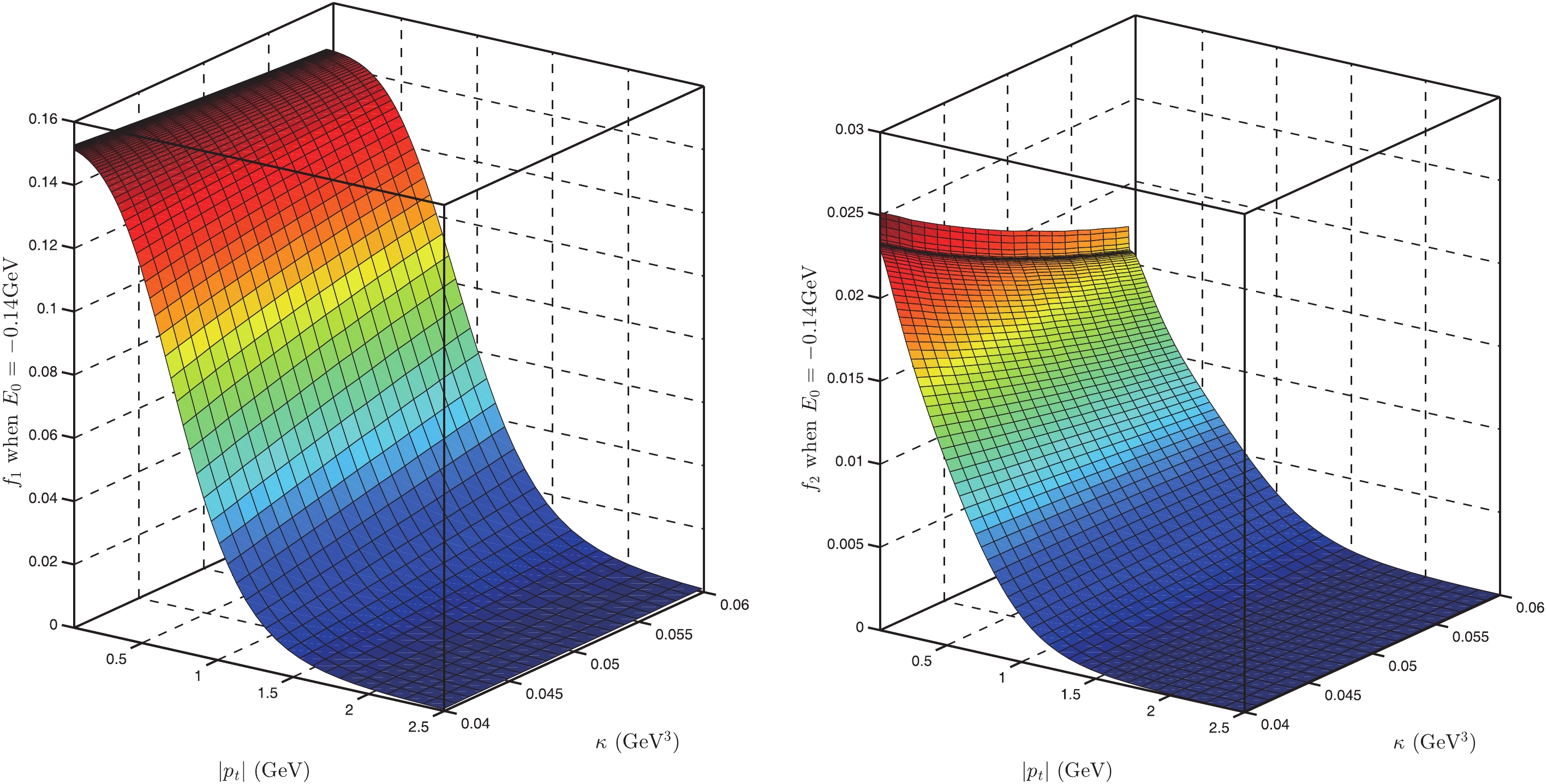Figure3. (color online) The BS wave functions for $ \Lambda $ with $ E_0=-0.14 $ GeV.

Figure4. (color online) The BS wave functions for $ \Lambda $ with $ E_0=-0.09 $ GeV.

Figure5. (color online) The BS wave functions for $ \Lambda $ with $ \kappa = -0.05 $ GeV³.

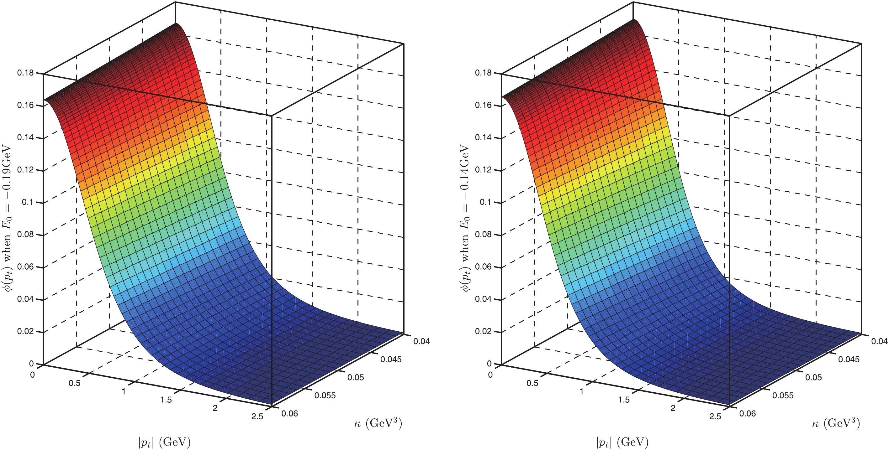Figure6. (color online) The BS wave function for $ \Lambda_b $ with $ E_0 = -0.19 $ GeV, $ E_0 = -0.14 $ GeV.

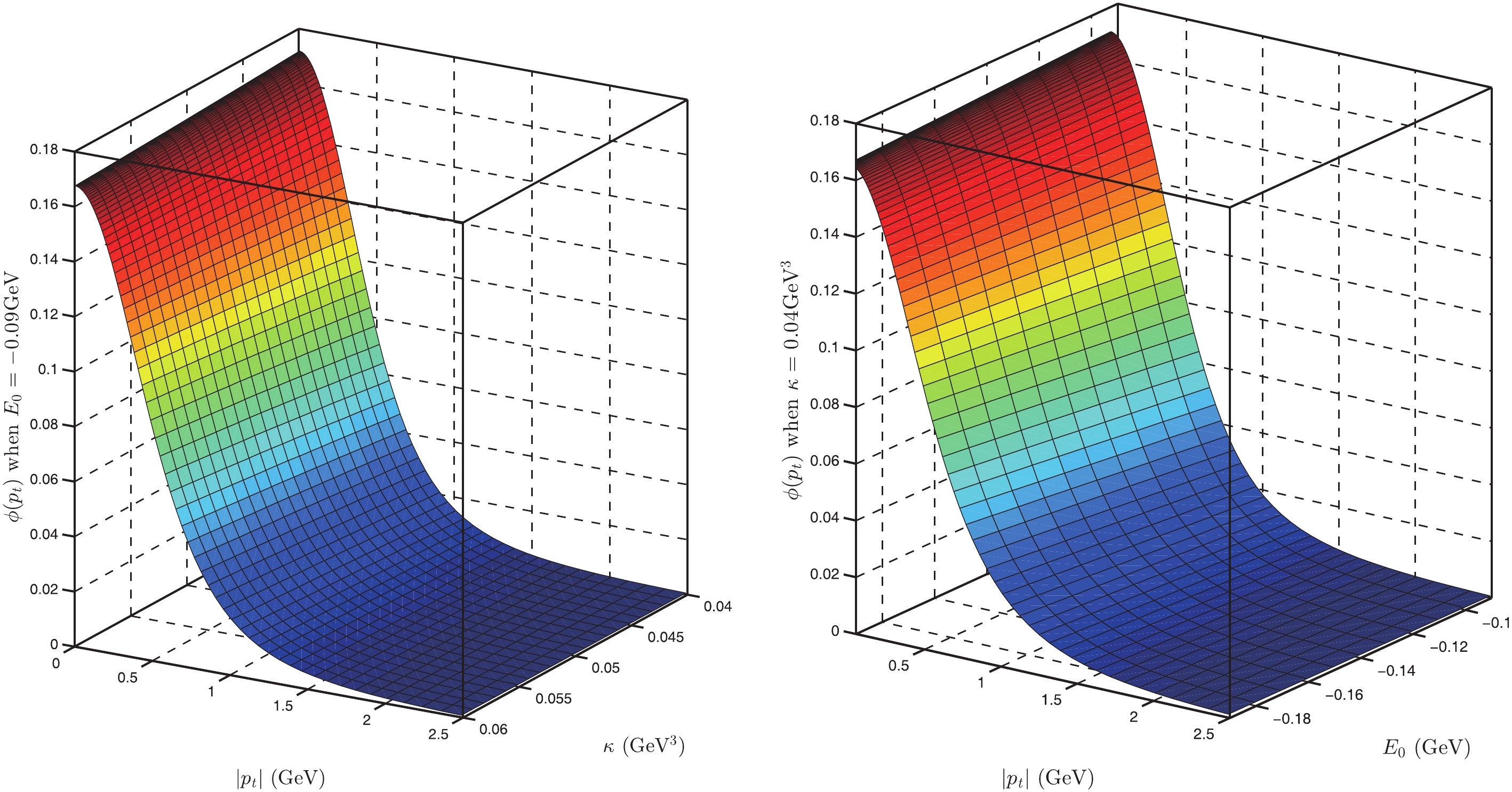Figure7. (color online) The BS wave function for $ \Lambda_b $ with $ E_0 = -0.09 $ GeV, and $ \kappa = -0.05 $ GeV³.

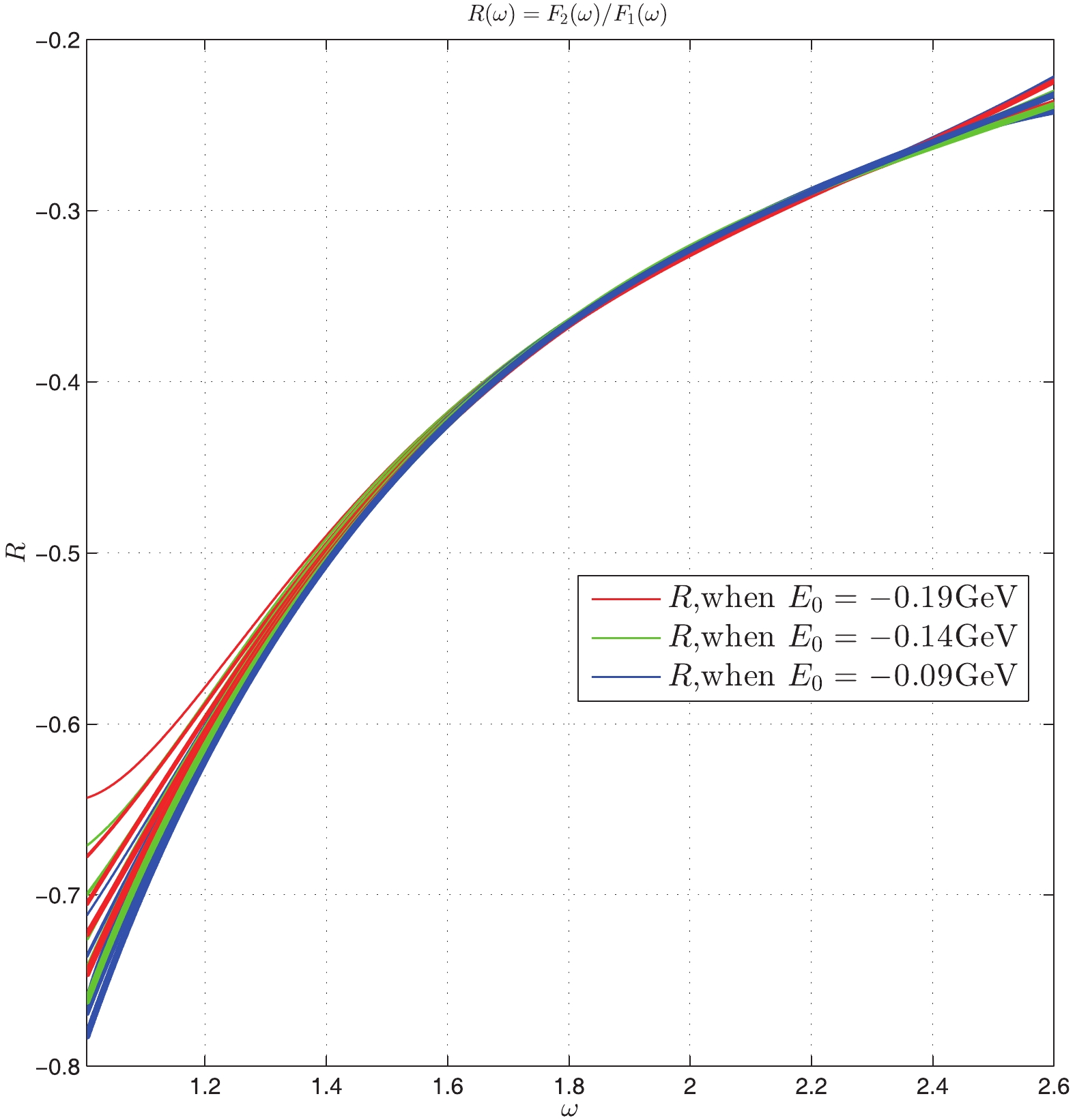Figure8. (color online) The values of $ R(\omega) $ for different binding energies $ E_0 $ and $ \kappa $ (the value of R decreases with increasing $ \kappa $, and with increasing $ \kappa $ the line thickens ($ \kappa $ from $ 0.040 $ to $ 0.060 $) for the same color line).

In Figs. 9-11, we show the $ \omega $-dependent differential decay width of $ \Lambda_b \rightarrow \Lambda l^- l^+(l = e, \mu, \tau) $ for different parameters. In our optimal range of parameters and in the range $ \kappa = 0.050 \pm 0.005 $ GeV³, and $ E_0 = -0.14 \pm 0.5 $ GeV, we obtain the branching ratios, respectively, which are listed in Table 3. From this table, we see that our results differ from those of the heavy quark effective theory (HQET) and QCD sum rules, but our results are consistent with the most recent experimental data. With $ \kappa = 0.045 \sim 0.055 $ GeV³ and $ E_0 = -0.19 \sim -0.14 $ GeV, we find ${\rm Br}(\Lambda_b \rightarrow \Lambda \mu^+ \mu^-)\times 10^6 = 0.602 \sim 1.48$, and in our optimal parameter range this value is $ 0.856\sim 1.039 $. The values of ${\rm Br}(\Lambda_b \rightarrow \Lambda e^+(\tau^+) e^-(\tau^-))\times 10^6$ in the above two ranges are $ 0.464\sim1.144\; (0.611\sim0.867) $ and $ 0.177\sim0.437\; (0.233\sim 0.331) $, respectively. When the parameters $ \kappa $ and $ E_0 $ vary in their regions, we find that the differential branching ratio of $ \Lambda_b \rightarrow \Lambda \mu^+ \mu^- $ does not peak at approximately $ \omega = 1.2 $. In [2, 3] when $ \omega $ in the range $ 1 \sim 1.4 $ (corresponding to $ q^2 $ in the range $ 15 \sim 20 $ GeV²), the experimental data exhibit a peak. Considering this difference, there could be new physics in this region.

$ -E_0 $($ \times 10^2 $ GeV) $ \kappa $($ \times 10^3 $ GeV3)	present work 1450±5	present work 14±550	HQET [55]	QCD sum rules [32]	Exp. [54]
$ Br( \Lambda_b\rightarrow \Lambda e^+ e^- ) \times 10^{6} $	0.464?1.144	0.611?0.867	2.23?3.34	4.6±1.6	?
$ Br( \Lambda_b\rightarrow \Lambda \mu^+ \mu^- )\times 10^{6} $	0.602?1.482	0.856?1.039	2.08?3.19	4.0±1.2	1.08±0.28
$ Br( \Lambda_b\rightarrow \Lambda \tau^+ \tau^- )\times 10^{6} $	0.177?0.437	0.233?0.331	0.179?0.276	0.8±0.3	?

Table3.The values of the branching ratios for $ \Lambda_b\rightarrow \Lambda l^+ l^- $ , and comparison with other models.

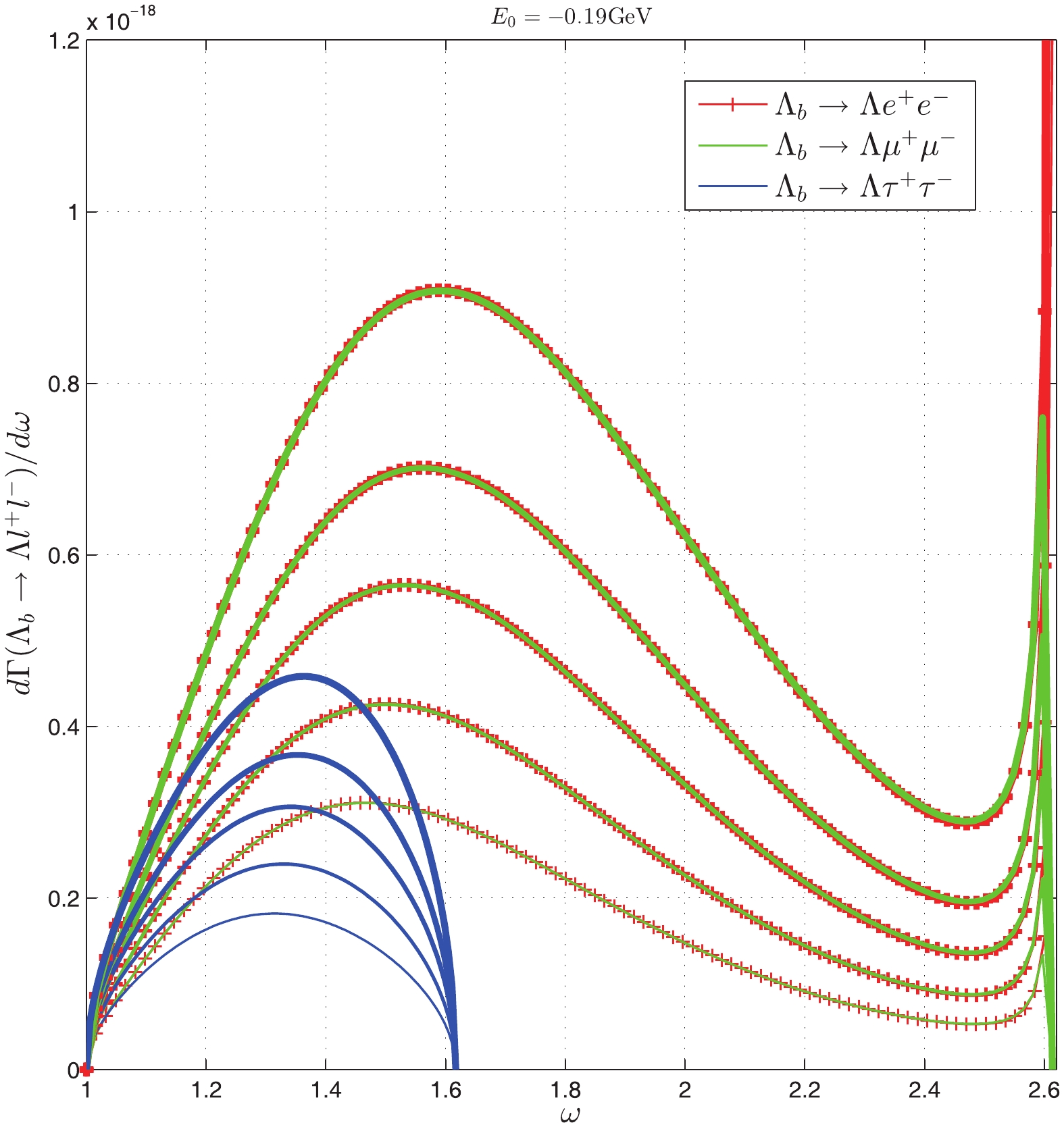Figure9. (color online) The differential decay width of $ \Lambda_b \rightarrow \Lambda l^+ l^- $ with the binding energy $ E_0 = -0.19 $ GeV (the decay width increases with increasing $ \kappa $ from $ 0.040 $ to $ 0.060 $ GeV³ for the same color line).

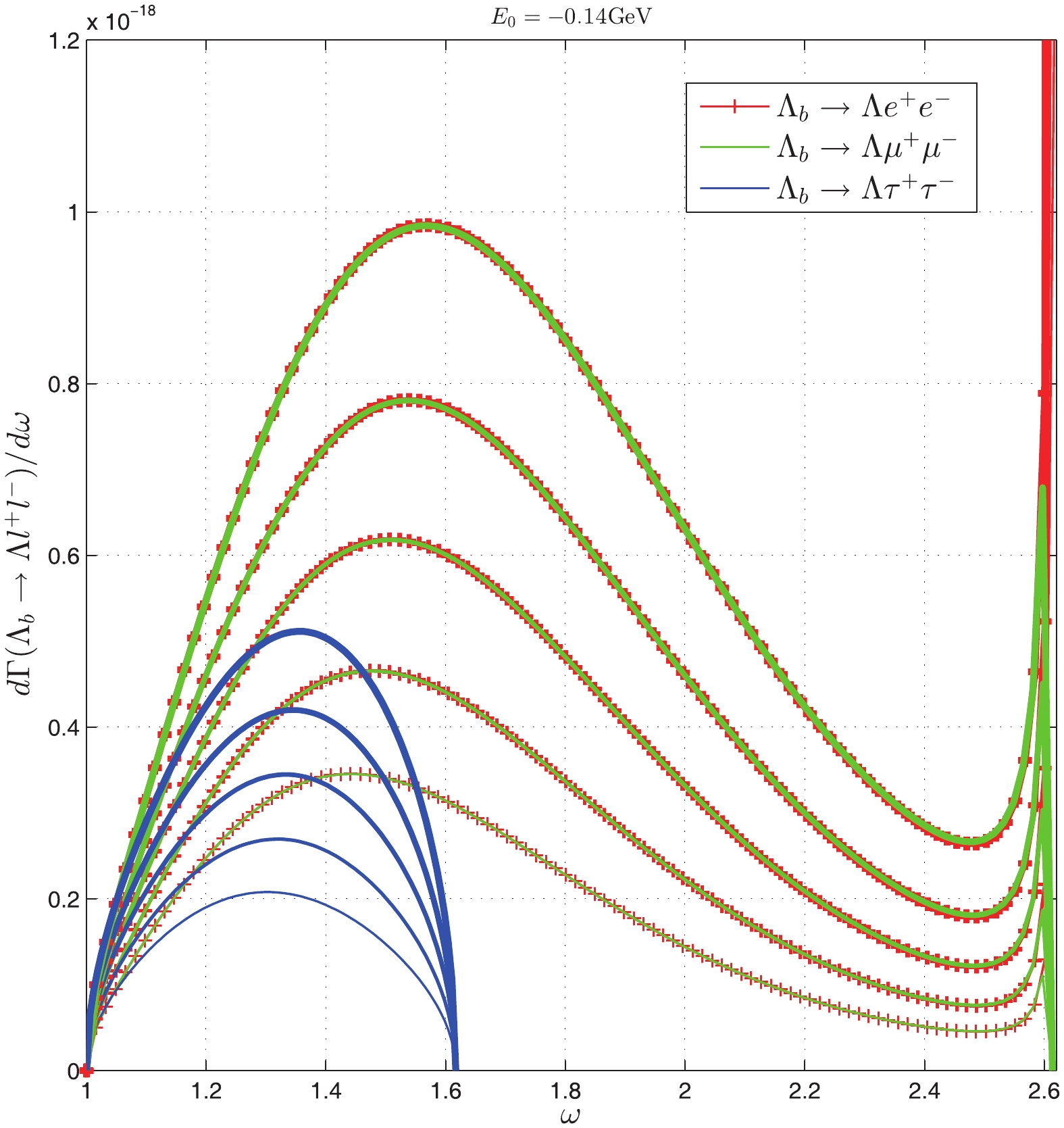Figure10. (color online) The differential decay width of $ \Lambda_b \rightarrow \Lambda l^+ l^- $ with the binding energy $ E_0=-0.14 $ GeV (the decay width increases with increasing $ \kappa $ from $ 0.040 $ to $ 0.060 $ GeV³ for the same color line).

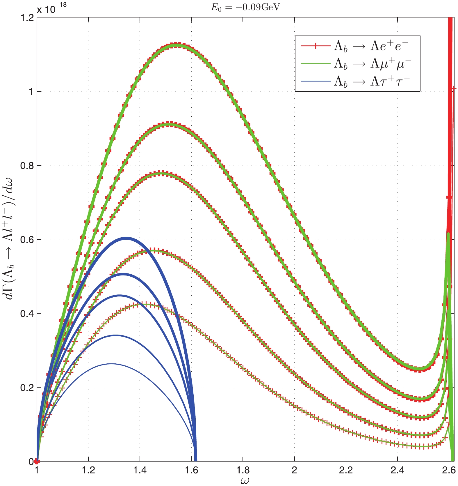Figure11. (color online) The differential decay width of $ \Lambda_b \rightarrow \Lambda l^+ l^- $ with the binding energy $ E_0 = -0.09 $ GeV (the decay width increases with increasing $ \kappa $ from $ 0.040 $ to $ 0.060 $ GeV³ for the same color line).

Theoretical studies of the decay $ \Lambda_b \rightarrow \Lambda l^+ l^- $ require knowing the matrix element $ \langle \Lambda| \bar{s} \Gamma b| \Lambda_b\rangle $. In the leading order in the HQET, this matrix element is given by two FFs. In the past few decades, in most of the published works the FFs were studied based on the QCD sum rules [12], and by fitting the available experimental data [31]. With experimental advances, the data pertaining to the $ \Lambda_b $ rare decay have been updated.
In the present work, we have performed the first BS equation calculation of these FFs. In our work, $ \Lambda_Q\; (Q = b,s) $ is regarded as a bound state of a Q-quark and a scalar diquark. In this picture, we established the BS equations for $ \Lambda_Q $, and derived the FFs for $ \Lambda_b \rightarrow \Lambda $ in the BS equation approach. After solving the BS equations of $ \Lambda $ and $ \Lambda_Q $, we calculated the ratio $ R = F_2/F_1 $ and the decay branching ratio for $ \Lambda_b \rightarrow \Lambda l^+ l^- $ , and compared our results with those reported in other works. We found that the shape of the differential decay branching ratio for $ \Lambda_b \rightarrow \Lambda \mu^+ \mu^- $ in our model is similar to the experimental data throughout most of the region, and in our work the shape of the decay differential branching ratio of $ \Lambda_b \rightarrow \Lambda l^+ l^-(l = e, \mu, \tau) $ agreed with the LQCD results [29, 46]. The experimental data for the differential decay width of $ \Lambda_b \rightarrow \Lambda \mu^+ \mu^- $ exhibited a peak with $ \omega \approx 1.2 $, but in most of the existing theoretical works such a pole does not appear. Therefore, new physics could exist in this region. More accurate experimental data should be obtained by repeated measurements in that region. Our result for $ \Lambda_b \rightarrow \Lambda \mu^+ \mu^- $ is very close to the experimental data, and we also provide predictions for the decays $ \Lambda_b \rightarrow \Lambda l^+ l^-(l = e, \tau) $, which need to be tested in future experiments. We find that for different parameters the ratio of FFs, $ R(\omega) $ changes from $ -0.80 $ to $ - 0.23 $ in our approach. This result agrees with the experimental data and with [12], and agrees with the LQCD results at $q^2_{\max}$ [46]. On the other hand, while using the BSE to investigate the octet and decuplet baryon properties in the ladder approximation, the quark exchanges generate the kernel when irreducible 3-quark interactions are neglected and separable 2-quark (diqaurk) correlations are assumed [56-58]. Then, both the scalar diquark current and axial-vector diquark current contributions are considered. We will also consider the axial-vector current contributions for the $ \Lambda_b\rightarrow \Lambda $ transition in future works.
In the HQET, the approximation $ 1/m_b \rightarrow \infty $ is uncertain within $\Lambda_{\rm QCD}/m_b$. Considering the uncertainties from the parameters $ E_0 $ and $ \kappa $ , the maximal uncertainty is approximately 22% in our optimal data region. In the future, our model will also be used to study the forward-backward asymmetries, T violation, and angular distributions in the decays induced by $ b \rightarrow s l^+ l^- $ , to further validate our FFs.