D*Dρ and B*Bρ strong couplings in light-cone sum rules - 中科院高能物理研究所

删除或更新信息，请邮件至freekaoyan#163.com(#换成@)

DDρ and BBρ strong couplings in light-cone sum rules

本站小编 Free考研考试/2022-01-01

濠电姷鏁搁崑鐐哄垂閸洖绠伴柟缁㈠枛绾惧鏌熼崜褏甯涢柣鎾寸☉椤潡鎳滃妤婁邯閹﹢鎮╃紒妯煎帾闂佸壊鍋呯换鍕春閿濆鐓欑€规洖娲ら埢鍫⑩偓瑙勬礃缁秹骞忛崨鏉戞嵍妞ゆ挾鍠愰蹇涙⒒閸屾艾鈧嘲霉閸ヮ灛娑㈠礋椤愩倖娈惧銈嗗坊閸嬫挻銇勯锝囩疄濠碘剝鎮傞崺鈩冩媴閾忕懓骞€濠碉紕鍋戦崐鏍偋濡ゅ懏鍋￠柕鍫濇穿婵娊鏌℃径濠勬皑婵℃彃鐗撻弻锟犲礃閿濆懍澹曟繝鐢靛О閸ㄦ椽鏁冮姀鐘垫殾闁告繂瀚弳鍡涙煕閺囥劌澧繛鍫濈焸濮婃椽宕ㄦ繝鍌毿曟繛瀛樼矌閸嬨倕鐣峰ú顏勭伋闁哄倶鍎查～宥夋⒑鐟欏嫬鍔ら柣掳鍔庢禍鎼侇敃閵堝洨锛滃┑掳鍊曢崯顐﹀几閺冨牊鐓欏瀣閳诲牊顨ラ悙鏉戠伌妤犵偛娲、娆撳传閸曨亣鍩呴梻鍌氬€风粈渚€骞栭锕€纾圭憸鐗堝笚閸嬶繝寮堕崼姘珕妞ゎ偅娲熼弻銊╂偆閸屾稑顏�
2濠电姷鏁搁崑鐐哄垂閸洖绠扮紒瀣紩濞差亜惟闁冲搫顑囩粙蹇涙⒑閸︻厼鍔嬫い銊ユ瀹曠敻鍩€椤掑嫭鈷戦柛娑橈工婵箑霉濠婂懎浠辩€规洘妞介弫鎾绘偐瀹曞洤骞楅梻渚€娼х换鍫ュ磹閺嵮€妲堢憸鏃堝蓟閿濆鐒洪柛鎰典簼閸ｎ厾绱撴担鍓插剰闁挎洦浜顐﹀磼閻愭潙娈愰梺鍐叉惈閸犳艾危閸楃偐鏀介柍钘夋娴滅偛顭胯椤ㄥ﹪寮€ｎ剛纾藉ù锝夋涧婵倸霉濠婂棗鐓愬ǎ鍥э功閳ь剚绋掕摫濠殿垰顕槐鎺戔槈濮楀棗鍓辩紓鍌氱Т閿曘儲绌辨繝鍥舵晝闁靛牆鎷嬮弳顓㈡⒑閸撹尙鍘涢柛銊ョ埣瀹曟椽鍩€椤掍降浜滈柟杈剧稻绾埖銇勯敂鑲╃暤闁哄本绋戦埢搴ょ疀閺囩媭鍞圭紓鍌欑窔缂傛艾螞閸曨喚浜欓梻浣告啞濞诧箓宕㈣ぐ鎺戠；闁圭儤顨嗛埛鎴︽煕濠靛棗顏╅柍褜鍓欑紞濠囧箖闁垮缍囬柍鍝勫亞濞肩喎鈹戦瑙掔懓鈻斿☉銏″剹婵°倐鍋撻柍瑙勫灴閹晠骞撻幒鍡椾壕闁归棿绀侀柨銈呪攽閻樻彃鏋ゆ繛鍫滅矙閺岋綁骞囬浣叉灆闂佹悶鍊楅崰鎰崲濠靛鐒垫い鎺戝閻掓椽鏌涢幇顖涚《闁活厽顨呴埞鎴︻敊缁涘鐣堕梺缁橆殔缁绘帞鍒掗崼鐔风窞閻庯綆鍓涢鏇㈡⒑閻熼偊鍤熷┑顔炬暬瀵娊鍩￠崒婊咁啎闁荤姴娉ч崟顐紦547闂傚倸鍊风粈浣革耿闁秲鈧倹绂掔€ｎ亞锛涢梺鐟板⒔缁垶鍩涢幒妤佺厱闁哄洦顨嗗▍鍛存煟韫囷絼閭柡宀嬬到铻栭悗锝庡亜椤忥拷4濠电姷鏁搁崑鐐哄垂閸洖绠扮紒瀣紩濞差亝鏅查柛銉㈡櫇椤︻垶姊洪悷閭﹀殶闁稿鍠栭崺銏ゅ籍閳ь剟濡甸崟顔剧杸闁规儳顕ˇ閬嶆⒑缁嬫鍎愰柟鐟版搐閻ｅ嘲顫滈埀顒勩€侀弮鍫濆耿婵°倕鍟獮鎰版⒒閸屾瑧顦﹂柛姘儏椤灝顫滈埀顒€鐣烽鐑嗘晝闁靛繈鍨哄▓楣冩⒑闂堟侗妾у┑鈥虫喘閸┿垽寮崼鐔哄幍闂佺顫夐崝鏇㈡儍濞差亝鐓熼柣鏃堟敱鐠愶紕绱掓潏銊ョ瑲鐎垫澘瀚埀顒婄秵娴滅偞绂掗悡搴樻斀闁绘劘娉涚槐锕傛煕濡ゅ嫭鐝ǎ鍥э功閳ь剚绋掕摫濠殿垱鎸抽幃宄扳枎濞嗘垵鍩屾繛瀛樼矒缁犳牠寮诲☉銏犵疀闁稿繐鎽滈弫鏍⒑缁洘娅旂紒缁樼箞瀵鈽夊⿰鍛澑闂佹寧绻傞幊搴綖閳哄懏鈷戦柛娑橈功閹虫洜绱掓潏銊︾妤犵偛绻橀幃鈺冩嫚閼碱剦鍟嬮梻浣告啞娓氭宕归幎鍓垮洭鍩￠崨顔规嫼闁荤偞绋堥埀顒€鍘栨竟鏇㈡⒒娴ｅ憡璐￠弸顏嗙磼閵娿劌浜圭紒顕呭幗瀵板嫰骞囬鐘插箻闂備礁鎼€氼剛鎹㈤幒鏃囧С闁圭ǹ绨烘禍婊堟煛閸ヮ煁顏堟倶閼碱兘鍋撳▓鍨珮闁稿锕ら锝囨崉鐞涒剝鐎婚梺璇″瀻閸忎勘鍊濆缁樻媴閻熼偊鍤嬬紓浣割儐閸ㄨ儻妫熷銈嗘尪閸ㄥ綊鎮為崹顐犱簻闁圭儤鍩婇弨濠氭倵濮樼偓瀚�40缂傚倸鍊搁崐椋庣矆娓氣偓钘濇い鏍ㄧ矌閻挾鈧娲栧ú銊х不閺冨牊鐓欓柟顖嗗苯娈堕梺宕囩帛濮婂綊骞堥妸銉建闁逞屽墰濞戠敻骞栨担鍛婄€柣搴秵娴滃爼鎮㈤崱娑欏仯闁搞儻绲洪崑鎾诲礂閸涱収妫滅紓鍌氬€峰ù鍥ㄣ仈閹间焦鍋￠柍鍝勬噹閽冪喓鈧厜鍋撻柛鏇ㄥ亞椤撴椽姊洪幐搴ｇ畵婵炶尙濞€瀹曟垿骞樼紒妯诲劒闁荤喐鐟ョ€氼剟宕㈣ぐ鎺撯拺闁告繂瀚婵嬫煕鎼淬垹鐏╂俊鍙夊姇楗即宕奸悢鍝勫妇闂備胶纭堕崜婵喢洪弽顐ュС缂侇偄瀵梻鍌氬€风欢姘缚瑜嶈灋闁哄啫鍊婚惌鍡椕归敐鍫殙闁荤喐瀚堥弮鍫濆窛妞ゆ棁顫夌€垫牠姊绘担鍛婂暈濞撴碍顨婂畷銏ゆ寠婢跺棙鐎洪悗鍏夊亾闁告洦鍓涢崢閬嶆⒑閸濆嫬鏆為柟绋垮⒔婢规洟骞愭惔娑楃盎闂侀潧楠忕槐鏇€€傞懠顒傜＜闁哄啫鍊搁弸娑欍亜閵忊剝绀嬮柟顔规櫊椤㈡洟锝為鐑嗘婵犵數鍋犻幓顏嗙礊閳ь剚銇勯銏╂█闁诡噯绻濋崺鈧い鎺戝閳锋帡鏌涚仦鎹愬闁逞屽厸缁瑩銆佸▎鎰瘈闁告洦鍓﹀ḿ鐔兼⒑閸撴彃浜濇繛鍙夌墱缁崵绱掑Ο闀愮盎闂佽宕樺▔娑㈩敁瀹€鍕厸濞达絽澹婇崕蹇斻亜椤撯剝纭堕柟椋庡█閸ㄩ箖宕楅崨顖涘瘻闂傚倷绶氶埀顒傚仜閼活垶宕㈤幖浣圭厾闁告劘灏欓崺锝呪攽閿涘嫭鏆柟顔界懇瀵爼骞嬮鐐搭啌濠电姵顔栭崰妤呮晝閳哄懎绀傛繛鎴炵椤洟鏌ㄥ┑鍡樺仾鐟滅増甯楅弲鏌ユ煕閳╁啰鎳呴柣鎾冲€搁—鍐Χ閸愩劎浠剧紒鐐緲缁夊墎鍒掗埡鍛亜缁炬媽椴搁弲婵嬫⒑闂堟稓澧曟繛璇х畵楠炲棝鏁愭径瀣ф嫼闂佸湱枪濞寸兘鍩ユ径瀣ㄤ簻闁挎棁顕у顕€鏌涢埞鎯т壕婵＄偑鍊栫敮鎺楁晝閵壯€鍋撳鐐28缂傚倸鍊搁崐椋庢閿熺姴纾诲鑸靛姦閺佸鎲搁弮鍫㈠祦闁告劦鍠栫粻濠氭煕閹捐尙绐旈柍鐟扮箲缁绘繈濮€閿濆棛銆愬Δ妤婁簼閹稿啿鐣峰┑瀣窛閻庢稒岣块崢閬嶆⒑閸濆嫬鏆婇柛瀣尵缁辨帞鈧綆鍋呭畷宀€鈧鍣崑濠囧箖娴犲鍨傛い鎰╁灩楠炴垿姊绘担鍛婃儓婵炶绠戦～婵嬪Ω閳哄倸浠梺瀹犳〃鐠佹彃危閸儲鐓欓柣鎰靛墯缂嶆垿鏌熼崗鍏煎€愰柡灞界Х椤т線鏌涢幘鍗炲妤犵偛绻橀弫鎾绘晸閿燂拷1130缂傚倸鍊搁崐椋庣矆娓氣偓钘濇い鏍ㄧ矌閻捇鏌涢幘鑼槮闁搞劍绻堥弻銊╂偄閸濆嫅銏㈢磼閳ь剟宕掗悙瀵稿幈濠电偞鍨堕敃顐﹀绩缂佹ḿ绠鹃柛顐ｇ箘閻掓悂鏌＄仦绋垮⒉鐎垫澘瀚埀顒婄秵娴滄粓锝為崶顒佲拺闂侇偆鍋涢懟顖涙櫠妤ｅ啯鐓欓柛鎴欏€栫€氾拷

Chao Wang ^1,,
, Hua-Dong Li ^2,3,,
,

Corresponding author: Chao Wang, chaowang@nankai.edu.cn

Corresponding author: Hua-Dong Li, lihd@ihep.ac.cn

1.School of physics, Nankai University, Weijin Road 94, Tianjin 300071, China
2.Institute of High Energy Physics, CAS, P.O. Box 918, Beijing 100049, China
3.School of Physics, University of Chinese Academy of Sciences, Beijing 100049, China
Received Date:2020-02-15
Available Online:2020-07-01
Abstract:We present an improved calculation of the strong coupling constants $ g_{D^*D\rho} $

and $ g_{B^*B\rho} $

in light-cone sum rules, including one-loop QCD corrections of leading power with $ \rho $

meson distribution amplitudes. We further compute subleading-power corrections from two-particle and three-particle higher-twist contributions at leading order up to twist-4 accuracy. The next-to-leading order corrections to the leading power contribution numerically offset the subleading-power corrections to a certain extent, and our numerical results are consistent with those of previous studies on sum rules. A comparison between our results and existing model-dependent estimations is also made.

HTML

--> --> -->

1.Introduction

This study aims to provide a more precise determination of $ D^*D\rho $ and $ B^*B\rho $ coupling in the framework of light-cone sum rules (LCSR). These couplings describe the low-energy interaction between heavy and light mesons, which are important in understanding QCD long-distance dynamics. The coupling is a fundamental parameter of the effective Lagrangian in heavy meson chiral perturbative theory (HM$ \chi $PT) [1-4], which plays an important role in the study of heavy meson physics. Phenomenologically, it describes the strength of the final state interactions [5], which are important in the generation of the strong phase in B decays [6,7]. Moreover, the coupling relates the pole residue of $ D(B) $ to $ \rho $ form factors at large momentum transfer by the dispersion relation, which is helpful to gain a better understanding of the behavior of form factors.
Various theoretical approaches have been suggested to evaluate the coupling. First, with the $ D(B) $ to $ \rho $ form factors obtained in a certain region of the momentum transfer from LCSR [8–10] and the lattice QCD [11], the corresponding pole residue that relates to the coupling is extracted with appropriate extrapolation of the form factors. The simplest approach to perform this extrapolation is the vector meson dominance (VMD) hypothesis, which neglects continuum spectral characteristics. In addition to the VMD approximation, certain other modified parameterizations for the form factors were proposed in [12-15]. In addition to the above method, the coupling can also be estimated from HM$ \chi $PT with the VMD approximation, as performed in [16-19].
Another strategy to obtain the strong coupling is calculation from first principles of QCD. We study the strong coupling constants $ g_{D^*D\rho} $ and $ g_{B^*B\rho} $ in LCSR using the double dispersion relation. The LCSR was proposed in [20-22] based on the light-cone operator-product-expansion (OPE) relative to the conventional QCD sum rules (QCDSR) method. There have been several studies addressing the couplings $ g_{D^*D\rho} $ and $ g_{B^*B\rho} $, starting from [23] with the inclusion of two-particle $ \rho $ DAs corrections up to twist-3 at leading order (LO). Years later, [24-27] improved the formal calculation by considering the two-particle twist-4 corrections [28] at LO. Meanwhile, $ g_{D^*D\rho} $ is also calculated with three-point QCDSR by taking into account the dimension-5 quark-gluon condensate corrections under flavor $ SU(3) $ symmetry [29]. In previous studies, coupling estimations showed a wide range of values. The results from LCSR studies [24-27] yield values that are smaller than those in other estimations; hence, we must perform a more accurate calculation to confirm whether this difference arises from radiative and power corrections. Moreover, the inclusion of NLO corrections can also decrease the scale-dependence. In this work, we present a calculation including $ {\cal{O}}(\alpha_s) $ corrections to the leading power contribution with the resummation of large logarithm to next-to-leading logarithmic accuracy (NLL). For the subleading-power corrections, our results also include the three-particle twist-4 corrections at LO.
The paper is organized as follows: in Section 2, we calculate the leading power contributions up to NLO. The procedures for analytic continuation and continuum subtraction are similar to the ones presented in [30,31]. Subleading-power corrections, including two-particle and three-particle corrections up to twist-4 at LO, are calculated in Section 3. Section 4 presents our numerical results and the phenomenological discussion. We summarize this work in the last section.

2.Leading power contributions

2.1.Hard-collinear factorization at LO in QCD

-->

2.1.Hard-collinear factorization at LO in QCD

The strong coupling constant $ g_{H^*H\rho} $ is defined by

$ \begin{array}{l} \langle\, \rho(p,\eta^*)\,H(q)\,|\,H^*(p+q,\varepsilon)\, \rangle = -g_{H^*H\rho}\, \epsilon_{pq\eta\varepsilon}\,, \end{array} $

(1)

with $ \epsilon_{pq\eta\varepsilon} = \epsilon_{\mu\nu\alpha\beta}\,p^\mu\,q^\nu\,\eta^{*\alpha}\,\varepsilon^\beta $. Here, we choose $ H^* $ and H to represent the $ D^{*-}(B^{*0}) $ meson and $ \bar{D}^{0}(B^+) $ meson, respectively, and $ \rho $ is $ \rho^- $. $ \varepsilon_{\mu} $ and $ \eta_\nu $ are the polarization vectors of $ H^* $ and $ \rho $ mesons, respectively. We use the conventions $ \epsilon_{0123} = -1 $ and $ D_{\mu} = \partial_\mu-{\rm i}\,g_s\,T^a\,A_\mu^a $. The couplings of different charge states are related by isospin symmetry, for example,

$ \begin{array}{l} g_{D^*D\rho}\equiv g_{D^{*-}\bar{D}^0\rho^-} = -\sqrt{2}\,g_{D^{*-}D^-\rho^0}\,. \end{array} $

(2)

We construct the following correlation function at the starting point

$ \begin{split} \Pi_\mu(p,q) = &\int {\rm d}^4x\,{\rm e}^{-{\rm i}(p+q)\cdot x}\langle\,\rho^-(p,\eta^*)\,|\,T\big\{\bar{d}(x)\,\gamma_{\mu \perp}\, Q(x),\\&\,\bar{Q}(0)\,\gamma_5\,u(0)\big\}\,|\,0\rangle\,, \end{split} $

(3)

where $ \gamma_{\mu\,\perp} = \gamma_{\mu}-\not\!{n}/2\,\bar{n}_\mu-\not\!{\bar{n}}/2\,n_\mu $, Q is the heavy quark field. We introduce two light-cone vectors $ n_\mu $ and $ \bar{n}_\mu $ with $ n\cdot n = \bar{n}\cdot \bar{n} = 0\,, n\cdot\bar{n} = 2 $. For the momentum, we choose a coordinate to have $ q_{\perp} = 0 $. Within the frame of the LCSR, the $ \rho $ meson is on the light-cone, and its momentum is chosen as

$ \begin{array}{l} p^{\mu} = \dfrac{n\cdot p}{2}\bar{n}_{\mu}\,. \end{array} $

(4)

On the hadronic level, taking advantage of the following definitions for decay constants

$ \begin{split} &\langle\,H^*(p+q,\varepsilon^*)\,|\,\bar{d}\,\gamma^\mu \,Q\,|\,0\,\rangle = f_{H^*}\,m_{H^*}\varepsilon^{*\mu}\,,\\& \langle\,0\,|\,\bar{Q}\,\gamma_5\,u\,|\,H(p)\,\rangle = -{\rm i}\,f_H\,\frac{m_H^2}{m_Q}\,, \end{split} $

(5)

the correlation function (4) can be written as

$ \begin{split} \Pi_\mu^{\rm had}(p,q) =& \frac{g_{H^*H\rho}\,f_{H^*}\,f_H}{[m_{H^*}^2-(p+q)^2-i\,0]\,[m_H^{2}-q^2-i\,0]}\, \frac{m_H^2\,m_{H^*}}{m_Q}\,\epsilon_{\mu pq\eta} \\ &+\iint_{\Sigma}\frac{\rho^h(s,s')\,{\rm d}s\,{\rm d}s'}{\left[s'-(p+q)^2\right](s-q^2)}+\cdots\,, \end{split} $

(6)

where the second term counts the contributions from higher resonances and continuum states. The ellipses denote the terms that vanish after the double Borel transformation.
After the double Borel transformation, we obtain the hadronic representation of the correlation function

$ \begin{split} \Pi_\mu^{\rm had}(p,q) =& \frac{f_H\,f_{H^*}\,m_H^2\,m_{H^*}}{m_Q}\,g_{H^*H\rho}\, {\rm e}^{-\frac{m_H^2+m_{H^*}^2}{M^2}} \epsilon_{\mu pq \eta} \\&+\iint_{\Sigma}\,{\rm d}s\,{\rm d}s'\,{\rm e}^{-\frac{s+s'}{M^2}}\,\rho^h(s,s')\,. \end{split} $

(7)

For the boundary of the integral $ \Sigma $, we take $ s+s' = 2\,s_0 $ with $ s_0 $ as the threshold of excited and continuum states. The Borel parameters associated with $ (p+q)^2 $ and $ q^2 $ are quite similar in magnitude; hence, we set the same value $ M^2 $.
On the quark level, the leading-twist tree diagram is displayed in Fig. 1. The correlation function reads

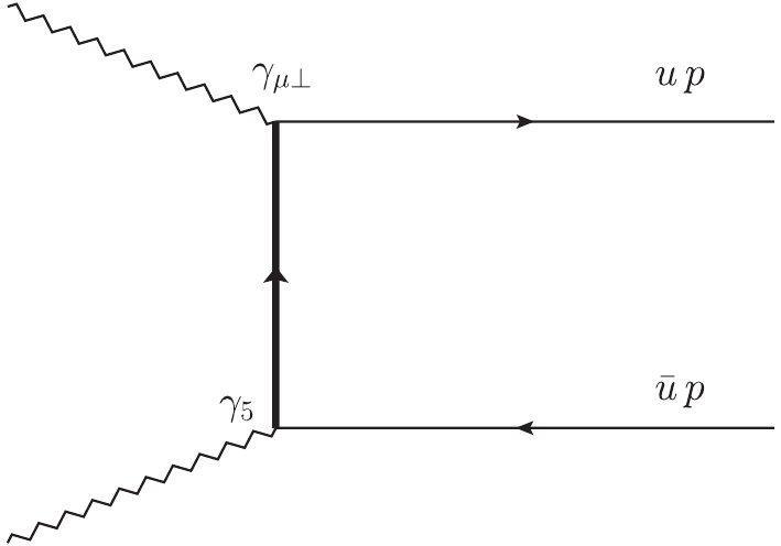Figure1. Diagram of leading-order (LO) contribution.

$ \begin{split} \Pi_\mu^{{\rm LT},(0)}(p,\,q) =& -\frac{\rm i}{2}\frac{\bar{n}\cdot q}{u\,q^2+\bar{u}\,(p+q)^2-u\,\bar{u}\,m_\rho^2-m_Q^2}\, \\&\times\bar{q}(u\,p)\,\gamma_{\mu\,\perp}\,\not\!\!{n}\,\gamma_5\,q(\bar{u}\,p)\\ =& -\frac{\rm i}{2}\frac{\bar{n}\cdot q}{u\,q^2+\bar{u}\,(p+q)^2-m_Q^2}\,\\&\times \bar{q}(u\,p)\,\gamma_{\mu\perp}\,\not\!\!{n}\,\gamma_5\,q(\bar{u}\,p)\\&+{\cal{O}}\left(\frac{\Lambda^2_{\rm QCD}}{m_Q^2}\right)\,. \end{split} $

(8)

Using the definition of the leading-twist $ \rho $ DA [28] in Appendix A, we obtain the leading twist tree level factorization formula

$ \begin{split} \Pi_{\mu}^{{\rm LT},(0)}(p,\,q)\!=\! -\!f_\rho^T(\mu)\,\epsilon_{\mu p q\eta}\!\int_0^1\!\! {\rm d}u\,\phi_\perp(u,\mu)\,\dfrac{1}{u\,q^2\!+\!\bar{u}\,(p\!+\!q)^2\!-\!m_Q^2}\,. \end{split} $

(9)

The result (9) can be written in the form of double dispersion relation

$ \begin{split} \Pi_{\mu}^{{\rm LT},(0)}(p,\,q) =& -f_\rho^T(\mu)\,\epsilon_{\mu p q\eta}\iint {\rm d}s\,{\rm d}s'\,\\&\times\frac{\rho^{\rm LT,(0)}(s,s')}{[s-q^2]\,[s'-(p+q)^2]}\,, \end{split} $

(10)

where the double dispersion density $ \rho^{\rm LT,(0)} $ is defined as

$ \begin{split} \rho^{{\rm LT},(0)}(s,s') = \frac{1}{\pi^2}\,{\rm Im}_{s'}\,{\rm Im}_{s} \int_0^1 {\rm d} u\,\frac{\phi_\perp(u,\mu)}{u\,s+\bar{u}\,s'-m_Q^2}\,. \end{split} $

(11)

The expression of wave function $ \phi_\perp(u,\mu) $ in terms of Gegenbauer polynomials can be written as

$ \begin{array}{l} \phi_\perp(u,\mu) = 6\,u\,\bar{u}\,\displaystyle\sum\limits_{n = 0}^{\infty}a_n^\perp(\mu)\,C_n^{3/2}(2u-1) = \displaystyle\sum\limits_{k = 1}^\infty b_k\,u^k\,, \end{array} $

(12)

where $ b_k $ is the function of Gegenbauer moments $ a(\mu) $. The spectral density can be obtained as follows [30]

$ \begin{split} \rho^{{\rm LT},(0)}(t,v) =& \displaystyle\sum\limits_{k = 1}^\infty b_k\,\frac{1}{\pi^2}\,{\rm Im}_{s'}\,{\rm Im}_{s}\int_0^1 {\rm d}u\,\frac{u^k}{u\,s+\bar{u}\,s'-m_Q^2} \\ =& \displaystyle\sum\limits_{k = 1}^\infty b_k\,\frac{(-1)^{k+1}}{k!}\,\frac{1}{2^{k+1}\,t}\,\left(\frac{m_Q^2}{t}-\bar{v}\right)^k\, \delta^{(k)}\left(v-\frac{1}{2}\right)\,\\&\times\theta(v\,t-m_Q^2)\,. \end{split} $

(13)

We defined two variables $ t = s+s', v = \frac{s}{s+s'} $ in Eq. (13), which are similar to those in our previous study [32].
Equating (6) and (10) and applying the double Borel transformation, then subtracting the continuum states using the quark-hadronic duality, we obtain the leading-twist strong coupling constant at LO

$ \begin{split} g^{{\rm LT},(0)} =& \dfrac{m_Q}{f_H\,f_{H^*}\,m_H^2\,m_{H^*}}\,f_\rho^T(\mu)\,\frac{M^2}{2}\, \phi_\perp\Big(\frac{1}{2},\mu\Big)\, \\&\times\Big[{\rm e}^{\textstyle\frac{m_H^2+m_{H^*}^2-2m_Q^2}{M^2}}-{\rm e}^{\textstyle\frac{m_H^2+m_{H^*}^2-2s_0}{M^2}} \Big]\,. \end{split} $

(14)

2.2.Next-to-leading order corrections

-->

2.2.Next-to-leading order corrections

The one-loop diagrams are shown in Fig. 2. The loop calculations are similar to those in [32]. We borrow the results from [32] and take the asymptotic form of wave function in Eq. (12) as $ \phi_\perp(u) = 6\,u\,\bar{u} $ for feasibility of calculation. Subsequently, we adopt a similar procedure to derive the double dispersion spectral densities and apply the double Borel transformation and continuum subtraction to obtain the result. Here, we omit the detailed procedures for simplicity, and the explicit operations with final results are provided in our previous study [32].

Figure2. NLO QCD corrections of leading-twist contributions.

Combing the NLO result from [32] with Eq. (14), we obtain the leading-twist sum rules up to $ {\cal{O}}(\alpha_s) $, and the coupling constant reads

$ \begin{split} g^{{\rm LT}} =& -\frac{m_Q}{f_H\,f_{H^*}\,m_H^2\,m_{H^*}}\, {\rm e}^{\frac{m_H^2+m_{H^*}^2}{M^2}}\, f_\rho^T(\mu)\,\\&\times \Big[-\frac{M^2}{2}\,\phi_\perp\Big(\frac{1}{2},\mu\Big)\,\big( {\rm e}^{-\frac{2m_Q^2}{M^2}} -{\rm e}^{-\frac{2s_0}{M^2}}\big) + {\cal{F}}^{{\rm LT},(1)}\Big]\,, \end{split} $

(15)

where

$ \begin{split} {\cal{F}}^{{\rm LT},(1)} =& \dfrac{\alpha_s\,C_F}{4\,\pi}\,\Big\{m_Q^2\int_{0}^{2\hat{s}_0-2}{\rm d}\sigma\, {\rm e}^{-\frac{\sigma+2}{\hat{M}^2}}\,g(\sigma) \\&+\Delta\,g(\hat{M}^2,m_Q^2)\Big\}\,, \end{split} $

(16)

and

$ \begin{split} g(\sigma) =& 3\,{\rm Li}_2(-\sigma)+3\,{\rm Li}_2(-\sigma-1)-6\,{\rm Li}_2\left(-\frac{\sigma}{2}\right) -3\,\ln\frac{\sigma}{2}\ln\frac{\sigma+2}{2}\\&+3\,\ln(\sigma+1) \,\ln(\sigma+2) -\frac{6\,(\sigma+1)^2}{(\sigma+2)^3}\,\ln (\sigma+1) \\&+ \frac{3\,(7\,\sigma^3+50\,\sigma^2+100\,\sigma+64)}{4\,(\sigma+2)^3}\,\ln\frac{\sigma}{2} \\&+ \frac{3}{2}\,\ln\frac{\sigma+2}{2} +\frac{3\,(11\,\sigma^2+28\,\sigma+24)}{8\,(\sigma+2)^2}\\&-3\,\ln\frac{\mu^2}{m_Q^2} -\frac{9}{4}\,\ln\frac{\nu^2}{\mu^2}-\frac{\pi^2}{4}\,, \\ & \Delta\,g(\hat{M}^2,m_Q^2) = 3\,\left(4+3\,\ln\frac{\mu^2}{m_Q^2}\right)\, m_Q^2\,{\rm e}^{-\frac{2m_Q^2}{M^2}}\,. \end{split} $

(17)

For the scale dependence, we use

$ \begin{split} \frac{\rm d}{{\rm d}\ln\mu}m_Q(\mu) =& -6\frac{\alpha_sC_F}{4\pi}m_Q(\mu)\,, \\ \frac{\rm d}{{\rm d}\ln\mu}f_\rho^T(\mu) =& -2\frac{\alpha_sC_F}{4\pi}f_\rho^T(\mu)\,, \end{split} $

(18)

and we obtain

$ \begin{array}{l} \dfrac{\rm d}{{\rm d}\ln\mu}g^{\rm LT} = 0+{\cal{O}}(\alpha_s^2)\,, \end{array} $

(19)

It is evident that our result is independent of the factorization scale $ \mu $ at the one-loop level.

4.Numerical analysis

4.1.Input parameters

-->

4.1.Input parameters

The masses of quarks in the $ \overline{\rm MS} $ scheme and the values of decay constants are listed in Table 1. The parameters in $ \rho $ DAs are listed in Table 2, which are extracted from the method of QCDSR [9,28].

$ \overline{m}_c(\overline{m}_c) $/GeV	$ \overline{m_b}(\overline{m}_b) $/GeV	$ f_\rho $/MeV	$ f_\rho^T(\mu_0) $/MeV	$ f_D $/MeV	$ f_{D^*} $/MeV	$ f_B $/MeV	$ f_{B^*} $/MeV
$ 1.288\pm0.02 $	$ 4.193_{-0.035}^{+0.022} $	$ 213\pm5 $	$ 160\pm7 $	$ 209.0\pm2.4 $	$ 225.3\pm 8.0 $	$ 192.0\pm4.3 $	$ 182.4\pm 6.2 $

Table1.Heavy quark masses [34,35] and decay constants [9,36-38], with scale-dependent quantity $ f_\rho^T $ given at $ \mu_0 = 1.0 $ GeV.

$ a_2^\parallel(\mu_0) $	$ a_2^\perp(\mu_0) $	$ \zeta_3(\mu_0) $	$ \omega_3^A(\mu_0) $	$ \omega_3^V(\mu_0) $	$ \omega_3^T(\mu_0) $	$ \zeta_4^T(\mu_0) $	$ \tilde{\zeta}_4^T(\mu_0) $	$ \langle\langle Q^{(1)}\rangle\rangle(\mu_0) $	$ \langle\langle Q^{(3)}\rangle\rangle(\mu_0) $	$ \langle\langle Q^{(5)}\rangle\rangle(\mu_0) $
$ 0.17\pm0.07 $	$ 0.14\pm0.06 $	$ 0.032\pm0.010 $	$ -2.1\pm1.0 $	$ 3.8\pm1.8 $	$ 7.0 \pm 7.0 $	$ 0.10\pm0.05 $	$ -0.10 \pm 0.05 $	$ -0.15\pm0.15 $	$ 0 $	$ 0 $

Table2.Non-perturbative parameters in DAs at scale $ \mu_0 = 1.0 \; {\rm GeV}. $

The solution to the two-loop evolution of the Gegenbauer moment $ a_n^\perp(\mu) $ is

$ \begin{split} f_\rho^T(\mu)\,a_n^\perp(\mu) =& \Big[ E_{T, n}^{\rm NLO}(\mu, \mu_0)+\frac{\alpha_s(\mu)}{4\pi} \,\sum\limits_{k = 0}^{n-2}\, E_{T, n}^{\rm LO}(\mu,\mu_0)\,\\&\times d_{T, n}^{k}(\mu,\mu_0) \Big]\,f_\rho^T(\mu_0)\,a_n^\perp(\mu_0)\,, \end{split} $

(27)

where the explicit expressions of $ E_{T,n} $ and $ d_{T,n} $ can be found in [39]. The scale evolution of other non-perturbative parameters to leading logarithmic accuracy is listed in Appendix B.
The factorization scales are taken as $ \mu_c\in[1,\,2] $ GeV around the default choice $ m_c $ and $ \mu_b = {m_b}^{+m_b}_{-m_b/2} $ for radiative $ D^* $ and $ B^* $ decays, respectively. For the Borel mass $ M^2 $ and the threshold parameter $ s_0 $, we assume the following intervals [40,41]

$ \begin{split}& \left\{ \begin{array}{l} s_0 = 6.0\pm0.5 \; {\rm GeV}^2\,,\\ M^2 = 4.5\pm1.0 \; {\rm GeV}^2\, , \end{array} \right. {\rm for} \; D^*\,D\,\rho\,;\\& \left\{ \begin{array}{l} s_0 = 34.0\pm1.0 \; {\rm GeV}^2\,,\\ M^2 = 18.0\pm3.0 \; {\rm GeV}^2\, , \end{array} \right. {\rm for}\; B^*\,B\,\rho\,, \end{split} $

(28)

which satisfy the standard criterions [42].
2

4.2.Theory predictions

-->

4.2.Theory predictions

The coupling constants for $ D^*D\rho $ and $ B^*B\rho $ are listed in Table 3. It is apparent that the perturbative QCD corrections decrease the tree level leading power contributions of coupling constants by 10% and 20% for $ D^*D\rho $ and $ B^*B\rho $, respectively. Meanwhile, contributions from tree level sub-leading power corrections have evident compensation effects, which increase the leading twist contributions by approximately 20% and 30% for $ D^*D\rho $ and $ B^*B\rho $, respectively. We also note that three-particle sub-leading power corrections have more minor effects compared with two-particle sub-leading power corrections, particularly for the coupling of $ B^*B\rho $, which is consistent with the validity of OPE.

	$ g^{\rm LT,LL} $	$ g^{\rm LT,NLL} $	$ g^{\rm 2P,LL} $	$ g^{\rm 3P,LL} $	Total
$ D^*\,D\,\rho $	$ 3.61_{-0.47}^{+0.54} $	$ 3.18_{-0.43}^{+0.53} $	$ 0.47_{-0.16}^{+0.17} $	$ 0.14_{-0.08}^{+0.09} $	$ 3.80_{-0.45}^{+0.59} $
$ B^*\,B\,\rho $	$ 3.59_{-0.43}^{+0.55} $	$ 2.91_{-0.42}^{+0.38} $	$ 0.96_{-0.15}^{+0.23} $	$ 0.022_{-0.012}^{+0.013} $	$ 3.89_{-0.48}^{+0.52} $

Table3.Results of $ g_{H^*H\rho} $ ($ {\rm GeV}^{-1} $). $ g^{\rm LT, LL} $ corresponds to the tree-level leading power contributions with resummation at LL accuracy; $ g^{\rm LT, NLL} $ corresponds to the leading power contributions up to NLO with resummation at NLL accuracy; $ g^{\rm 2P, LL} $ and $ g^{\rm 3P, LL} $ are from 2-particle and 3-particle sub-leading power corrections at LO separately.

The uncertainties are also included for separate terms of coupling constants in Table 3. The uncertainties are estimated by varying independent input parameters, and the individual uncertainties are presented in Table 4. To estimate total uncertainties, we add them in quadrature to obtain the final results. From Table 4, we can see that the primary uncertainties stem from the Borel mass $ M^2 $ and parameter $ a_2^\perp $ both for $ D^*D\rho $ and $ B^*B\rho $. The second Gegenbauer moment $ a_2^\perp $ refers to transversely polarized $ \rho $ meso twist-4 LCDA, which is indicated in Appendix A, B. The quasi-distribution amplitudes (quasi-DAs), which are based on the large-momentum effective theory (LaMET) [43,44], along with the simulation from lattice QCD [45] are also capable of extracting meson LCDA [46,47] other than QCDSR. In the future, a more precise determination of the $ \rho $ meson LCDA will be helpful to decrease the uncertainties of couplings.

	Central value	$ \Delta\, f_{H^*} $	$ \Delta\, m_{Q} $	$ \Delta\, M^2 $	$ \Delta\, \mu $	$ \Delta\, f_\rho^T $	$ \Delta\, a_2^\perp $
$ g_{D^*D\rho} $	$ 3.80_{-0.45}^{+0.50} $	$ ^{+0.14}_{-0.13} $	$ ^{+0.00}_{-0.01} $	$ ^{+0.38}_{-0.20} $	$ ^{+0.20}_{-0.01} $	$ \pm0.11 $	$ \pm 0.32 $
$ g_{B^*B\rho} $	$ 3.89_{-0.48}^{+0.52} $	$ ^{+0.14}_{-0.13} $	$ ^{+0.12}_{-0.08} $	$ ^{+0.36}_{-0.23} $	$ ^{+0.14}_{-0.26} $	$ \pm0.12 $	$ \pm 0.24 $

Table4.Central value and individual uncertainty of $ g_{H^*H\rho} $ ($ \rm{GeV}^{-1} $) due to variations in input parameters. We only list numerically significant uncertainties.

Next, we compare our results of coupling constants with those obtained in other studies using sum rules, as shown in Table 5. Among them, the LCSR studies [24,26] did not take the perturbative QCD corrections and 3-particle corrections into account, and the QCDSR study considers the dimension-5 quark-gluon condensate corrections [29]. As mentioned above, the NLO effects of leading power almost cancel the subleading-power corrections; hence, it is expected that our results are close to those of previous sum rules studies within the errors.

	This work	LCSR [24]	LCSR [26]	QCDSR [29]
$ g_{D^*D\rho} $	$ 3.80_{-0.45}^{+0.50} $	$ 4.17\pm1.04 $	$ 3.56\pm0.60 $	$ 4.07\pm0.71 $
$ g_{B^*B\rho} $	$ 3.89_{-0.48}^{+0.52} $	$ 5.70\pm1.43 $	–	–

Table5.Numerical values of coupling constants $ g_{H^*H\rho} $ ($ \rm{GeV}^{-1} $) from several studies via sum rules.

Next, we extract the $ B^*B\rho $ coupling from form factors. The $ B\to\rho $ form factors $ V(q^2) $ and $ T_1(q^2) $, which are related to $ g_{B^*B\rho} $, are defined as

$ \begin{split} &\langle\,\rho^-(p,\eta^*)\,|\,\bar{d}\,\gamma_\mu\,b\,|\,B^-(p+q)\,\rangle = \frac{2}{m_B+m_\rho}\,V(q^2)\,\epsilon_{\mu\eta pq}\,, \\& \langle\,\rho^-(p,\eta^*)\,|\,\bar{d}\,i\,\sigma_{\mu\nu}\,q^\nu\,b\,|\,B^-(p+q)\,\rangle = -2\,T_1(q^2)\,\epsilon_{\mu\eta pq}\,. \end{split} $

(29)

From the dispersion relation of the form factor $ F_i(q^2) $

$ \begin{split} F_i(q^2) = \frac{r_1^i}{1-q^2/m_{B^*}^2}+\int_{(m_B+m_\rho)^2}^\infty \frac{\rho(s)}{s-q^2-{\rm i}\epsilon}\,, \end{split} $

(30)

the strong coupling relates to the pole of the form factors at the unphysical point $ q^2 = m_{B^*}^2 $. Then, we have the relation

$ \begin{split} r_1^V = &\lim_{q^2\to m_{B^*}^2} \big(1-q^2/m_{B^*}^2\big)\,V(q^2) = \frac{m_B+m_\rho}{2\,m_B^*}\,f_{B^*}\,g_{B^*B\rho}\,, \\ r_1^{T_1} =& \lim_{q^2\to m_{B^*}^2} \big(1-q^2/m_{B^*}^2\big)\,T_1(q^2) = \frac{1}{2}\,f_{B^*}^T\,g_{B^*B\rho}\,, \end{split} $

(31)

where $ f_{B^*}^T $ is the tensor coupling of the $ B^* $ meson, and it is defined as

$ \begin{array}{l} \langle\,0\,|\,\bar{b}\,\sigma_{\mu\nu}\,q\,|\,B^*(q,\epsilon)\,\rangle = {\rm i}\,f_{B^*}^T\,(\epsilon_\mu\,q_\nu-\epsilon_\nu\,q_\mu)\,. \end{array} $

(32)

Using Eq. (31) and choosing the size $ f_{B^*}^T = f_{B^*} $, we extract several numerical values of the coupling $ g_{B^*B\rho} $ from recent LCSR studies [9,10], which we list in Table 6.

This work	$ V(q^2) $ [9]	$ T_1(q^2) $ [9]	$ V(q^2) $ [10]	$ T_1(q^2) $ [10]
$ 3.89_{-0.48}^{+0.52} $	$ 8.50\pm1.73 $	$ 8.02\pm1.59 $	$ 6.04_{-2.34}^{+1.30} $	$ 7.25^{+1.72}_{-2.78} $

Table6.Coupling $ g_{B^*B\rho} $ ($ \rm{GeV}^{-1} $) from the residue of $ B\to\rho $ form factor V and $ T_1 $ in LCSR fit and compared to our result.

As shown, our central value is smaller than the extrapolations from LCSR form factors. To explain this discrepancy, on the one hand, uncertainties from the parameterizations of form factors to obtain the un-physical singularity may be underestimated. On the other hand, for the double dispersion relation, the Borel suppression is not sufficient to neglect the isolated excitation contributions, according to the discussion in [48]. Apart from $ B \to \rho $, the $ B^* \to B $ and $ B^* \to \rho $ form factors can also be used to extract the coupling. To the best of our knowledge, there are no relevant studies that address corresponding form factors in LCSR. A future study could verify whether different choices of form factors are consistent across the coupling extractions.
Finally, we analyze our study and compare it with other model-dependent studies. The HM$ \chi $PT effective Lagrangian to parametrize the $ H^*HV $ coupling can be written as [1]

$ \begin{array}{l} {\cal{L}}_V = {\rm i}\,\lambda\,{\rm Tr}[{\cal{H}}_b\,\sigma^{\mu\nu}\,F_{\mu\nu}(\rho)_{ba}\,\bar{{\cal{H}}}_a]\,, \end{array} $

(33)

with

$ \begin{array}{l} F_{\mu\nu}(\rho) = \partial_\mu\, \rho_\nu-\partial_\nu\, \rho_\mu +[\rho_\mu,\,\rho_\nu]\,, \quad \rho_\mu = {\rm i}\,\dfrac{g_V}{\sqrt{2}}\,\hat{\rho}_\mu\,, \end{array} $

(34)

where $ \hat{\rho} $ is a $ 3\times 3 $ matrix for light meson nonet, and the heavy $ H, H^* $ mesons are represented by the doublet field $ {\cal{H}}_a $ with the conventional normalization. The parameter $ g_V = m_\rho/f_\pi $. In the chiral and heavy quark limits, we have the following relation for the coupling $ \lambda $

$ \begin{array}{l} \lambda = \dfrac{\sqrt{2}}{4}\,\dfrac{1}{g_V}\,g_{H^*H\rho}\,. \end{array} $

(35)

We find the coupling $ \lambda = 0.23\pm0.03\,{\rm GeV}^{-1} $ at leading power from our value of $ g_{B^*B\rho} $.
In Table 7, we compare this value with other model estimations. Similar to the estimations from form factors, our result is smaller than the model predictions.

This work	VMD [19]	CQM [49]	CQM [50]	QM+VMD [51]
$ 0.23 $	$ 0.56 $	$ 0.60 $	$ 0.47 $	$ 0.33 $

Table7.Central value of coupling $ \lambda $ ($ \rm{GeV}^{-1} $) from model estimations compared to our result.

One possibility for this discrepancy may be that the model predictions have potentially larger errors. Consequently, in principle, the LCSR is more credible. However, in addition to the possible influences of excitation contributions mentioned above, the values of NLO corrections to higher twists and the sub-sub-leading power contributions are unknown, which may likewise represent sources of the discrepancy. Improvements in the calculations of both the sum rules and models may help better understand such discrepancies in the future.

5.Conclusion

We compute the $ D^*D\rho $ and $ B^*B\rho $ strong couplings to subleading-power in LCSR. Long-distance dynamics are incorporated in the $ \rho $ DAs. We calculate the $ {\cal{O}}(\alpha_s) $ corrections to leading power of the sum rules. The subleading-power corrections are calculated at LO by accounting the two- and three-particle wave functions up to twist-4. The analytical results of the double spectral densities are obtained, and in accordance with the previous study, we also perform a continuum subtraction for the higher-twist corrections. The LO results are independent of the choice of the duality region because of the special form of the double spectral density.
The NLO corrections reduce the numerical tree-level results by 10% and 20% for $ D^*D\rho $ and $ B^*B\rho $, respectively. However, the subleading-power corrections at LO can give rise to values about 20% and 30% for $ D^*D\rho $ and $ B^*B\rho $, respectively. Summing all the contributions, our values are consistent with the predictions from previous sum rules studies. Moreover, we also predict the coupling $ \lambda $ in HM$ \chi $PT at leading power. The central value of our result is smaller than the existing model-dependent estimations. Possible explanations for the discrepancy are potentially large errors within models and influences of excitation contributions in LCSR. Moreover, radiative corrections to higher twists and sub-sub-leading power contributions may also be sources of error. A better understanding of this discrepancy will prove beneficial to shedding light on long-distance QCD dynamics in the future.
We are grateful to Prof. Cai-dian Lü and Prof. Yue-long Shen for helpful discussions.