Guang-Lei Li ^,
, Chun-Bin Yang ^,
,

Corresponding author: Guang-Lei Li, ligl@mails.ccnu.edu.cn

Corresponding author: Chun-Bin Yang, cbyang@mail.ccnu.edu.cn

Institute of Particle Physics & Key Laboratory of Quark and Lepton Physics (MOE), Central China Normal University, Wuhan 430079, China
Received Date:2018-12-04
Available Online:2019-05-01
Abstract:A quark coalescence model, based on semi-relativistic molecular dynamics with color interactions among quarks, is presented and applied to pp collisions. A phenomenological potential with two tunable parameters is introduced to describe the color interactions between quarks and antiquarks. The interactions drive the process of hadronization that finally results in different color neutral clusters, which can be identified as hadrons based on some criteria. A Monte Carlo generator PYTHIA is used to generate quarks in the initial state of hadronization, and different values of tunable parameters are used to study the final state distributions and correlations. Baryon-to-meson ratio, transverse momentum spectra, pseudorapidity distributions and forward-backward multiplicity correlations of hadrons produced in the hadronization process, obtained from this model with different parameters, are compared with those from PYTHIA.

HTML

--> --> -->

In high energy physics, perturbative Quantum Chromodynamics (pQCD) has achieved remarkable success in describing hard processes with large momentum transfers due to the fact that partons behave like they were nearly free, so that the interactions can be calculated perturbatively. However, pQCD is invalid in the long distance regime where the momentum transfers are low. In this confinement regime, partons with color are converted into color neutral hadrons through the hadronization process, which is still not possible to solve from first principles due to its non-perturbative nature. Thus, some phenomenological models are often needed to describe the dynamical features of non-perturbative QCD, e.g. the Lund string fragmentation model [1-5] used in PYTHIA [6, 7], the cluster model used in HERWIG [8, 9], coalescence models [10-13] used in the Monte Carlo transport models such as AMPT [14] and PACIAE [15-17], etc. The Lund model is based on the assumption of linear confinement supported by lattice QCD. In this model, the flux-tube of strong color field between a color charge and its anticolor charge is represented by a relativistic string which produces a linear confinement potential. The fragmentation process is described by the dynamics of relativistic strings, while the production of quark-antiquark or diquark-antidiquark pairs is modeled as a tunneling process. The cluster model is based on the assumption of pre-confinement. Gluons are split into quark-antiquark or diquark-antidiquark pairs after a parton shower, followed by the formation of color-singlet clusters which may decay isotropically into hadrons. Coalescence models connect quark numbers and pre-hadron numbers by assuming an underlying coalescence with some phase space constraint.
The molecular dynamics (MD) method [18, 19] is a microscopic many body approach, which has been successful in materials science, chemical physics and biomolecules [20-22]. It has the advantage of being able to solve various problems without many assumptions. To study the microscopic dynamics of quark matter during the hadronization process dominated by non-perturbative QCD, methods of MD simulation have been applied in recent years [23-30]. Ref. [23] studied the hermalization process of a strongly interacting quark matter. Ref. [24] used quantum molecular dynamics to study the quark phase transition of a quark system at finite density. A relativistic molecular dynamics approach based on Nambu-Jona-Lasinio (NJL) Lagrangian [31] was applied in Ref. [25] to study the evolution of high energy heavy ion collisions. The NJL model, as a low energy approximation to the QCD theory, has been applied to study the properties of baryon-rich matter [32-34]. A quark molecular dynamics based on a non-relativistic approach was used to describe hadronization of an expanding quark gluon plasma in heavy ion collisions with particle creation taken into consideration in Refs. [26, 27]. Refs. [28, 29] analyzed the properties of quark matter at finite baryon densities and zero temperature by using a semi-classical constrained molecular dynamics approach.
In this paper, we study the hadronization process microscopically using a quark coalescence model in the framework of the semi-relativistic molecular dynamics method. In this model, quarks are treated as particles moving synchronously with relativistic velocities and interacting through a potential, which leads to hadronization of quarks. The implementation of the model is based on the work in [30] and a generalized form of the Cornell potential used in that paper. In Refs. [26, 27], the Cornell potential was also applied by using the classical molecular dynamics to yield colorless clusters. However, the details of implementation, such as the determination of the color factor, initial state, algorithm, criteria to end the evolution, hadron identification etc., are different from ours. Our study is preliminary and focuses on the effects of different parameters on the final state properties of hadrons by analyzing the variations of baryon-to-meson ratio, transverse momentum spectra, pseudorapidity distributions and forward-backward multiplicity correlations with different values of parameters.
This paper is organized as follows. In Section 2, the phenomenological potential and related dynamics are discussed. Its application to hadronization is described in Section 3 for quarks produced by PYTHIA in pp collisions. The obtained final state distributions and correlations are presented in Section 4. A discussion is given in the last section.

2

-->

2.1.Interaction potential

In our study, a Cornell-like phenomenological potential [35-37] is employed with some free parameters. The Cornell potential has gained success in describing the properties of bound states, especially heavy quark mesons [37-40]. It is parametrized as a linear combination of the Coulomb and linear potentials. The Coulomb term, similar in behavior to the electromagnetic case, is responsible for the one-gluon exchange between two quarks, while the linear term dominates when the distance is large and thus gives rise to confinement. In this paper, quarks and antiquarks are treated as particles interacting through this kind of potential depending on their distance and color combination. The potential between a pair of quarks i and j separated by a distance $ r_{ij} $ is defined as

${V_{ij}} = {\alpha _{ij}}\left(a{r_{ij}} - \frac{b}{{{r_{ij}}}}\right) + c,$

(1)

where a, b are coefficients that describe the strength of interactions, c is a constant, and $ \alpha_{ij}=\alpha_{ji} $ is a color factor determined by the combination of color charges of these two quarks (red, green or blue for quarks, and their anticolors for antiquarks). The units for a, b, and c are GeV/fm, GeV·fm, and GeV, respectively.
This paper regards a and b as adjustable parameters, which correspond to the string tension and phenomenological strong coupling constant, respectively. Note that the unit of b is GeV·fm, which needs to be converted to get the usual dimensionless coupling constant, e.g. b=0.1 GeV·fm $ \approx 0.508 $. However, considering that our main concern is the influence of the change of a and b on the hadronization process, their absolute values are not relevant. We set a>0. For given a and b, c can be determined by assuming that the total potential energy between all pairs of quarks and antiquarks in the initial state is zero, so as to conserve the total energy.
The value of the color factor $ \alpha_{ij} $ for a combination of color charges includes two parts: the sign of the combination of color charges and the relative strength of the color factor.
The sign of $ \alpha_{ij} $ for a color combination can be determined by considering different kinds of combinations of quarks carrying color charges. For a quark and antiquark, if they carry a color charge and its anticolor charge, respectively, they can form a color neutral meson and should attract each other, and thus $ \alpha_{ij}>0 $; otherwise, the force interacting between them is repulsive, and $ \alpha_{ij}<0 $. For two quarks (or antiquarks), if their colors are different, they may form a diquark (or an antidiquark) , their interaction is attractive and $ \alpha_{ij}>0 $; otherwise their interaction is repulsive and $ \alpha_{ij}<0 $.
The next step is the determination of relative strengths of $ \alpha_{ij} $ for different combinations of color charges. The net force acting from a hadron with neutral color on a quark or antiquark should be zero if the hadron can be regarded as a point particle. Suppose that this force is a result of the offset of forces from quarks composing the hadron, then the relative strength of different combinations of color charges can be determined by comparing the forces acting from quarks in a meson or baryon on the outside quark (or antiquark). For a quark and antiquark comprising a meson, their colors must be complemented. If the color charge of the outside quark is the same as that of a quark inside the hadron, then the force acting from the same color quark on the outside quark is repulsive, and the force acting from the antiquark inside the meson is attractive. One then concludes that the absolute value of the relative strength of $ \alpha_{ij} $ between the combination of same color charges and the one with complemented color charge is 1:1. If the color charge of the outside quark is different and with non-complementary color to that of a quark inside a meson, the absolute value of the relative strength of attraction between different color charges and the repulsion between non-complemented color charges is also 1:1. (The same results can be obtained by supposing an antiquark on the outside). In the case of a quark outside a baryon composed of three quarks, the color of the outside quark must be the same as that of one quark in the baryon, and different from the other two, then the relative strength of the repulsive force between quarks of the same color should be twice the attractive force between quarks with different colors. Other combinations can be considered likewise. In this way, the relative strength between different combinations of color (or anticolor) charges can be deduced. Finally, combining with the signs of $ \alpha_{ij} $, the relative values of $ \alpha_{ij} $ are summarized in Table 1.

$ \alpha_{ij} $	r	g	b	$ \overline{r} $	$ \overline{g} $	$ \overline{b} $
r	?1	$ \frac{1}{2} $	$ \frac{1}{2} $	1	$ -\frac{1}{2} $	$- \frac{1}{2} $
g	$ \frac{1}{2} $	?1	$ \frac{1}{2} $	$- \frac{1}{2} $	1	$ -\frac{1}{2} $
b	$ \frac{1}{2} $	$ \frac{1}{2} $	?1	$- \frac{1}{2} $	$- \frac{1}{2} $	1
$ \overline{r} $	1	$ -\frac{1}{2} $	$ -\frac{1}{2} $	?1	$ \frac{1}{2} $	$ \frac{1}{2} $
$ \overline{g} $	$ -\frac{1}{2} $	1	$ -\frac{1}{2} $	$ \frac{1}{2} $	?1	$ \frac{1}{2} $
$ \overline{b} $	$ -\frac{1}{2} $	$- \frac{1}{2} $	1	$ \frac{1}{2} $	$ \frac{1}{2} $	?1

Table1.The color factor $ \alpha_{ij} $ for different combinations of color charges.

The color factors deduced here are the same as those in Refs. [26, 27], which are obtained from the Lagrangian for one-gluon exchange in QCD interactions.
2 -->

2.2.Dynamics

Since it is hard to describe the microscopic dynamics of a relativistic many body system in a relativistically consistent way [41, 42], in this paper we treat quarks and antiquarks as particles whose motion is driven by the forces they exert on each other. For a system consisting of quarks and antiquarks, the color charges of quarks (or antiquarks) are fixed as an approximation. Additionally, gluons are not considered as particles in the model, but are accounted for in the background field of the system.
It should also be noted that the relativistic effects, such as retardation and chromomagnetism should be taken into account, since most quarks in our simulation are light quarks. However, because of many difficulties for a many-particle system, these are not included in our present work. Additionally, since the proper time of each particle in the system is different, the choice of the reference frame is also an issue. In our study, we only consider the time with respect to the laboratory frame (i.e. the center-of-mass frame of the pp collision), and assume that all quarks and antiquarks interact synchronously.
The motion of quarks and antiquarks in the system is influenced by their mutual interaction. From Eq. (1), one can get the force acting on quark i from quark j,

$\overrightarrow {{F_{ij}}} = - \nabla {V_{ij}} = - {\alpha _{ij}}\left(a\frac{{{{\vec r}_{ij}}}}{{|{{\vec r}_{ij}}|}} + b\frac{{{{\vec r}_{ij}}}}{{|{{\vec r}_{ij}}{|^3}}}\right),$

(2)

and the total force acting on quark i from the other quarks and antiquarks in the system is

$\overrightarrow {{F_i}} = \sum\limits_{j \ne i} - {\alpha _{ij}}\left(a\frac{{{{\vec r}_{ij}}}}{{|{{\vec r}_{ij}}|}} + b\frac{{{{\vec r}_{ij}}}}{{|{{\vec r}_{ij}}{|^3}}}\right).$

(3)

The non-covariant equations of motion for quark i are

$\left\{ \begin{split}&\displaystyle\frac{{{\rm d}{{\vec r}_i}}}{{{\rm d}t}} = {{\vec v}_i},\\&\displaystyle\frac{{{\rm d}{{\vec p}_i}}}{{{\rm d}t}} = {{\vec F}_i},\\&{{\vec v}_i} = \displaystyle\frac{{{{\vec p}_i}}}{{\sqrt {{m_i}^2 + {{\vec p}_i}^2} }}.\end{split} \right.$

(4)

Eqs. (1) and (2) have no meaning if $ r_{ij} \to 0 $. To avoid this situation, Ref. [23] introduced a short-distance cutoff, i.e. for $ r_{ij} < 0.1 \rm \ fm $ the potential was taken as a linear function of r, which was explained as a result of the finite spatial extension of the quark wavefunction. Our model sets a minimum distance $ r_{\rm min}=0.1 \rm \ fm $ between quarks. A “contact” interaction occurs if the distance between quarks i and j is less than $ r_{\rm min} $ as they approach each other. The interaction between them is implemented by assuming that the force is along the line connecting the two quarks. (If there are more than two quarks with a distance less than $ r_{\rm min} $, one can let the two quarks with a minimum distance have a “contact” interaction and bounce back first, and consider the other pairs accordingly). As a result, the components of momenta perpendicular to $ \vec{r}_{ij} $ are unchanged after a collision, whereas the components of momenta parallel to $ \vec{r}_{ij} $ can be solved by considering the conservation of energy and momentum [42, 43],

$\begin{split}\vec p_{i,\parallel }' =& \gamma {({{\vec v}_{cm}})^2}[2{{\vec v}_{cm}}{E_i} - (1 + |{{\vec v}_{cm}}{|^2}){{\vec p}_{i,\parallel }}],\\E_i' =& \gamma {({{\vec v}_{cm}})^2}[(1 + |{{\vec v}_{cm}}{|^2}){E_i} - 2{{\vec v}_{cm}} \cdot {{\vec p}_{i,\parallel }}],\end{split}$

(5)

where the variables with superscript′ denote variables after collision, and $ \vec{v}_{cm}=(\vec{p}_{i,\parallel}+\vec{p}_{j,\parallel})/(E_i+E_j) $ is the collision invariant velocity of the center-of-mass of these two quarks.
2 -->

2.3.Integration method

The molecular dynamics simulation is performed by dividing the evolution time into a large number of time-steps. For each step, the force acting on each quark and the velocity of each quark are regarded as constant, and the position and momentum for the next time step can be calculated according to Eq. (4) by using some kind of integration method. In this way, as the time step advances, the position and momentum of each quark are updated, and the process can be repeated.
Apparently, if the time-step is too large, the integration error is large, which leads to a relatively large error of dynamical properties and energy drift. On the other hand, if the time-step is too small, the cost of simulation will be too large, because updating the positions and momenta of all quarks for each step, and especially updating of forces, is time-consuming. For each step, to update the forces one needs to calculate the relative distances between all pairs of quarks, which is quite time-consuming if the number of quarks is large. Thus, the integration algorithm is vital to the accuracy and efficiency of simulation.
The velocity Verlet algorithm [18] is adopted in our model, considering that its accuracy is of the order of two (which is better than the usual Euler method), and it consumes less memory since each iterative step just needs the properties of the preceding step. In addition, it only requires to update the forces once for each step.
Suppose that the position, momentum, kinetic energy (rest energy included) of quark i at time t are $ \vec{r}_i(t) $, $ \vec{p}_i(t) $, $ E_i(t) $, the force acting on it is $ \vec{F}_i(t) $, and the timestep is $ \delta t $. The corresponding values at the next step $ t+\delta t $ can be determined as follows. The momentum of quark i at $ t+\displaystyle\frac{1}{2}\delta t $ is

${\vec p_i}\left(t + \frac{1}{2}\delta t\right) = {\vec p_i}(t) + \frac{1}{2}\delta t{\vec F_i}(t),$

(6)

from which one can get the velocity at $ t+\displaystyle\frac{1}{2}\delta t $,

${\vec v_i}\left(t + \frac{1}{2}\delta t\right) = \frac{{{{\vec p}_i}\left(t + \displaystyle\frac{1}{2}\delta t\right)}}{{\sqrt {m_i^2 + {{\vec p}_i}{{\left(t + \displaystyle\frac{1}{2}\delta t\right)}^2}} }}.$

(7)

Then the position at $ t+\delta t $ can be written as

${\vec r_i}(t + \delta t) = {\vec r_i}(t) + {\vec v_i}\left(t + \frac{1}{2}\delta t\right)\delta t.$

(8)

After the update of the position of each quark, the forces acting on each quark at $ t+\delta t $ can be obtained using Eq. (3), which can be used to calculate the momentum at $ t+\delta t $

${\vec p_i}(t + \delta t) = {\vec p_i}\left(t + \displaystyle\frac{1}{2}\delta t\right) + \displaystyle\frac{1}{2}\delta t{\vec F_i}(t + \delta t).$

(9)

In this way, the coordinates and momenta of quarks in a system are advanced by one time-step $ \delta t $.

One can apply the potential model above to study the process of hadronization for quark systems produced by PYTHIA for pp collision at different energies using the molecular dynamics method. PYTHIA 8.230 is used in the calculation.
2

-->

3.1.Initial state

The initial state of quarks for a pp collision event is generated with the Monte Carlo generator PYTHIA [6, 7].
PYTHIA is a simulation program that can be used to generate events in high-energy collisions between two incoming particles (e.g. pp, ep and $ e^{+}e^{-} $). It is based on a series of analytical results and a coherent set of models based on QCD from a few body hard process to a multiparticle final state. Its physics features consist of hard and soft interactions, initial/final-state showers, beam remnants, multiple parton interactions, fragmentation and decay. PYTHIA version 8.2 [7] , used in our model, is a complete rewrite from Fortran to C++ and can be used for experimental or phenomenological studies, especially for the LHC studies. A pp collision is decomposed into parton-parton collisions in this model, which can be divided into soft and hard collisions, where the hard part is described by the lowest leading order perturbative QCD, whereas the soft part is considered empirically.
Hadrons produced directly by hadronization in PYTHIA (i.e. hadrons before decay) are input in our model as “parent hadrons” and their identities are coded according to the “The Monte Carlo particle numbering scheme” [44] used in PYTHIA. They are then decomposed into quarks and antiquarks, according to the flavors and spins of their valence quarks. A meson is converted into a quark and antiquark, while a baryon (or antibaryon) is first converted to a quark and diquark (or an antiquark and antidiquark), and the latter are then broken into quarks (or antiquarks). This decomposition is assumed to be isotropic in the rest frame of the parent hadron. The implementation of the decomposition is the same as in the diquark break-up method in Ref. [15]. This approach of obtaining the initial state is similar to that in AMPT with string melting [14]. The decomposition of “parent hadrons” is equivalent to keeping the evolution process at the parton level until all quarks and antiquarks are produced in the string fragmentation process in PYTHIA.
The sum of color charges of quarks from the same hadron is kept neutral, so that the whole system is also color neutral.
The masses of quarks and antiquarks during the decomposition are taken to be the current masses used in PYTHIA, e.g. $ m_d=0.0099 \ {\rm GeV/c}^2 $, $ m_u=0.0056 \ {\rm GeV/c}^2 $, $ m_s=0.199 \ {\rm GeV/c}^2 $, $ m_c=1.23 \ {\rm GeV/c}^2 $, $ m_b=4.17 \ {\rm GeV/c}^2 $. The constituent masses are not used in this process because for a 0^- pseudoscalar meson, as the Goldstone boson, the mass may be smaller than the sum of masses of constituent quarks, which makes it impossible to convert these mesons into quarks.
After all hadrons from PYTHIA are decomposed, the initial state consisting of quarks and antiquarks is generated. The properties, like masses, flavors, colors, momenta of all quarks and antiquarks are determined. However, the positions are not as the information about the coordinates of parent hadrons from PYTHIA is not available.
We set the initial positions of quarks and antiquarks using a simple method as follows. First, we assume that the parent hadrons are uniformly distributed in a circle lying in a transverse plane with a zero longitudinal coordinate. This is similar to the assumption used in Refs. [45, 46] that a pp collision can be approximately regarded as a disc as a result of the Lorentz contraction in the laboratory frame. The circle radius is set to 1 fm. We then define the formation time $ t_{f} $ of one quark as the time it travels from the point where the parent hadron is generated to the position where it is decomposed from its parent hadron. The parent hadron moves along a straight trajectory with a constant velocity. This method sets the initial positions of quarks by introducing a formation time and using straight-line trajectories of their parent hadrons. It is similar to that in the AMPT model with string melting, but does not consider the transverse momentum dependence of the formation time. It also does not take into account the Lorentz boost effect on the formation time, otherwise the quarks with large momenta would be spaced too far apart. If the interactions in the system begin at this point, the quarks and antiquarks from the same hadron would immediately return to their original hadron combination. For this reason, we assume that quarks decomposed from parent hadrons do not interact until they have moved away during an additional time $ t_f^{'} $ with their respective constant velocities. $ t_f^{'} $ is referred to as the free flow time of quarks. The position of a parton at the beginning of evolution is then

${\vec r_i} = {\vec r_0} + {\vec v_h}{t_f} + {\vec v_q}t_f' = {\vec r_0} + \frac{{{{\vec p}_h}}}{{{E_h}}}{t_f} + \frac{{{{\vec p}_q}}}{{{E_q}}}t_f',$

(10)

where $ \vec{r}_0 $ is the initial position (whose longitudinal coordinate is zero) of the parent hadron.
Considering that quarks are formed at different stages during the pp collision process, we suppose that the formation time is a uniformly distributed random variable between 0 and the maximum formation time $ t_{f,\rm max} $. As revealed by the results presented below, the final distribution of hadrons is strongly influenced by the initial geometry of quarks. Given the absence of a sensible method for determining the initial coordinates, the method above is just used as a first attempt.
In fact, according to the calculations using the initial geometry above, the value of the parameter c in the interaction potential in Eq. (1) is much smaller than a and b (about two orders of magnitude smaller), especially for events with large quark multiplicity.
Two kinds of quark masses are used in our model. In addition to the current masses used during the decomposition of parent hadrons mentioned above, quark masses during the evolution process are taken to be the constituent masses, $ m_d=0.325\ {\rm GeV/c}^2 $, $ m_u=0.325 \ {\rm GeV/c}^2 $, $ m_s=0.5 \ {\rm GeV/c}^2 $, $ m_c=1.6 \ {\rm GeV/c}^2 $, $ m_b=5.0 \ {\rm GeV/c}^2 $. The current masses are changed into constituent masses of their respective quarks after decomposition. The difference between these two kinds of masses leads to the energy discrepancy due to the change of the rest energy of each quark, which is negligible compared with the energy of the collision system.
2 -->

3.2.Evolution and hadronization

Because the speed of a quark with a large momentum (e.g. over 100 GeV) is usually very close to the speed of light, its momentum is nearly equal to its energy in magnitude. Thus the change of momentum does not have much effect on the change of its velocity and it is quite hard to separate quarks into color neutral clusters with speeds very near to 1. Therefore, in our study the dynamics of high energy quarks (decomposed from parent hadrons with energy larger than 50 GeV) are excluded from the evolution simulation.
After removing high energy quarks, we use the Verlet method mentioned above to simulate the evolution of the quark system from a pp collision. The time-step is set to $ \delta t=0.005 \ \rm fm/c $. With such a time-step, it is found that the energy drift is less than 1% for almost all events.
After initialization, the system begins to evolve. The evolution of the system yields color neutral clusters of different sizes due to the interactions among quarks. A cluster is regarded as well separated from the others if the distance between the cluster and any other quark outside the cluster is larger than 2 fm. Once all quarks gather into clusters and the number and constituents of clusters do not change during 10 fm/c, the evolution process is considered to be finished. This treatment of hadronization is different from that in Refs. [26, 27], where a quark-antiquark pair (or three quarks or antiquarks) is regarded as a hadron when the interaction between the pair (or three quarks or antiquarks) and the rest of the system is weaker than a lower bound, and the formed hadron is removed from the system.
A small cluster containing one quark and one antiquark could be mapped as a meson, while a cluster composed of three quarks (or antiquarks) could be regarded as a baryon (or antibaryon). Occasionally, larger clusters containing more than three quarks may also form. These clusters can be regarded as multi-quark states, such as tetraquark and pentaquark. Since the relative motion among quarks in a multi-quark cluster is usually small (all with speed close to 1), if they happen to be close to each other, with short range interactions, it may be hard for them to be well separated into smaller clusters. Therefore, multi-quark states may survive for a long time during system evolution, and are allowed in our model. This is different from the requirement in Refs. [27, 30].
Figure 1 illustrates the quark spatial distributions for an event sample at three different points in time, with the evolution starting time set at t=0.
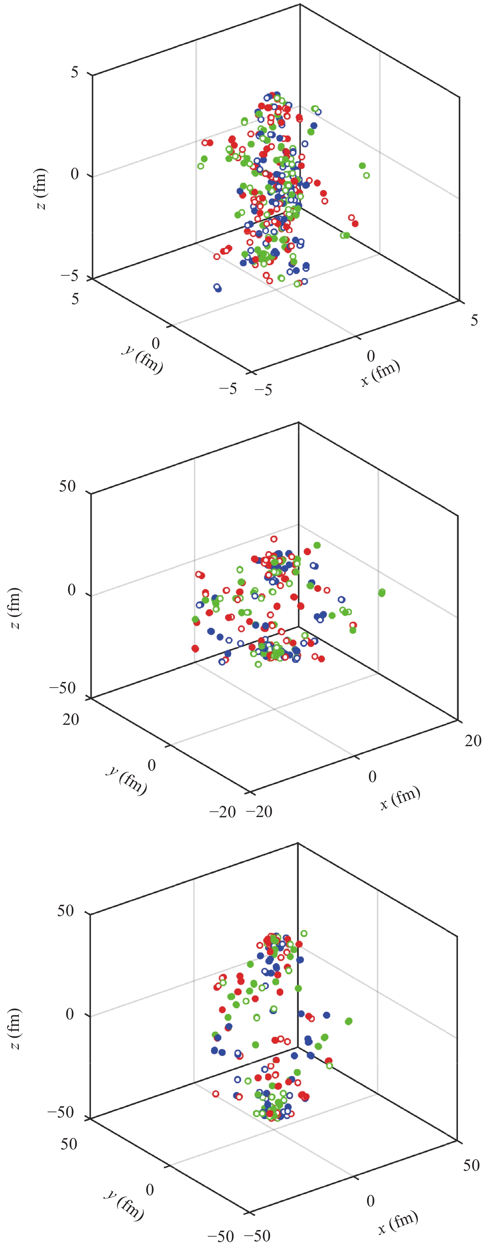Figure1. (color online) Evolution of a system with 382 quarks and antiquarks input from PYTHIA at three different points in time: t=0 (top panel), t=20 fm/c (middle panel) and t=40 fm/c (bottom panel). The solid and open circles represent quarks and antiquarks, respectively, whose colors correspond to the circles.

2 -->

3.3.Hadron identification

The mass $ m_h $ of a cluster is determined by its four-momentum,

$\begin{split}m_h^2 =& E_h^2 - \vec p_h^2\\ =& {\left(\displaystyle\sum\limits_i {\sqrt {m_i^2 + \vec p_i^2} + \displaystyle\frac{1}{2}\displaystyle\sum\limits_{i \ne j} {{V_{ij}}} } \right)^2} - {\left(\displaystyle\sum\limits_i {{{\vec p}_i}} \right)^2},\end{split}$

(11)

where the three momentum $ \vec{p}_h $ is the sum of the momenta of its constituent quarks, and energy $ E_h $ is the sum of the total energy, with i and j the numbers of quarks in the cluster.
Eq. (11) leads to the continuous invariant mass of a cluster, whereas the mass of the corresponding hadron is a discrete one, which is similar to the scenario in the quark coalescence of AMPT. In identifying a cluster as a hadron, the conservation of three-momentum is chosen. In other words, the three-momentum of an identified hadron is taken as that of the cluster, while its mass is chosen according to its identity. This process will cause a small change of energy of this hadron and of the system.
The criterion for hadron identification is similar to that in PACIAE and AMPT. Formed mesons with the same flavor composition may be a pseudoscalar meson or vector meson. If the invariant mass of a cluster with a quark and antiquark is nearer to that of a pseudoscalar meson, it is recognized as a pseudoscalar meson, otherwise it is a vector meson. The same principle is used in the identification of octet and decuplet baryons. As for the formation of flavor-diagonal mesons, the formation probabilities are considered, which can be determined as follows.
For flavor-diagonal clusters containing $ u \overline{u} $, $ d \overline{d} $, $ s \overline{s} $, the mixing angles are taken to be the same as used in PYTHIA [6], which give the wavefunctions of pseudoscalar mesons

$\left\{ \begin{split}&{\pi ^0} = \displaystyle\frac{1}{{\sqrt 2 }}(u\bar u - d\bar d),\\&\eta = \displaystyle\frac{1}{2}(u\bar u + d\bar d) - \displaystyle\frac{1}{{\sqrt 2 }}s\bar s,\\&\eta ' = \displaystyle\frac{1}{2}(u\bar u + d\bar d) + \displaystyle\frac{1}{{\sqrt 2 }}s\bar s,\end{split} \right.$

(12)

and vector mesons

$\left\{ \begin{split}&{\rho ^0} = \displaystyle\frac{1}{{\sqrt 2 }}(u\bar u - d\bar d),\\&\omega = \displaystyle\frac{1}{{\sqrt 2 }}(u\bar u + d\bar d),\\&\phi = s\bar s.\end{split} \right.$

(13)

We rewrite them to get the wavefunctions of $ u \overline{u} $, $ d \overline{d} $, $ s \overline{s} $ represented by pseudoscalar mesons,

$\left\{ \begin{aligned}&u\bar u = \displaystyle\frac{1}{2}(\eta + \eta ') + \displaystyle\frac{1}{{\sqrt 2 }}{\pi ^0},\\&d\bar d = \displaystyle\frac{1}{2}(\eta + \eta ') - \displaystyle\frac{1}{{\sqrt 2 }}{\pi ^0},\\&s\bar s = \displaystyle\frac{1}{{\sqrt 2 }}(\eta ' - \eta ),\end{aligned} \right.$

(14)

and by vector mesons

$\left\{ \begin{aligned}&u\bar u = \displaystyle\frac{1}{{\sqrt 2 }}(\omega + {\rho ^0}),\\&d\bar d = \displaystyle\frac{1}{{\sqrt 2 }}(\omega - {\rho ^0}),\\&s\bar s = \phi .\end{aligned} \right.$

(15)

We use the rule that if the invariant mass of a flavor diagonal cluster (i.e. $ u \overline{u} $, $ d \overline{d} $, or $ s \overline{s} $) is larger than $ 0.5 \ {\rm GeV/c}^2 $ it is a vector meson and its species is determined by the probabilities according to Eq. (15). Otherwise, it is a pseudoscalar meson and its species is determined by the probabilities according to Eq. (14).
Since the spins of quarks are not considered in the evolution, the differentiation between clusters composed of quarks with the same flavors is determined by their masses only. The exotic hadrons consisting of more than three quarks are not considered in the identification process.
Once a hadron is identified, an id code can be given to it, just as in the input procedure for initial state mentioned above. After the identification process, the id number, four-momentum, and mass of a hadron are known. The identified hadrons can then be input in PYTHIA to decay and to get stable hadrons (the “ProcessLevel” and “PartonLevel” in PYTHIA are switched off and only “HadronLevel” is used). Therefore, the final distribution of hadrons is influenced not only by the dynamics during the evolution process, but also by the decay which is determined by hadron identification (hence the mass of a cluster must be identified). As the main focus of our study is on the influence of the dynamics, the decay process is not considered, and only hadrons formed directly from hadronization are taken into consideration.

The main tunable parameters in our model are the interaction coefficients a and b in Eq. (1), which affect the evolution process, and maximum formation time $ t_{f,\rm max} $ and time $ t_{f}^{'} $ for free flow in Eq. (10), which determine the configuration of the initial state. By setting different parameters, the distributions and correlations of final state hadrons could vary. The influence of parameters is shown in the following numerical results from our model. About 150k non-single diffractive (NSD) events in pp collisions were generated for each combination of parameters to study their influence on the distributions and correlations.
2

-->

4.1.Baryon-to-meson ratio

Define $ N_B $ as the sum of multiplicities of newly produced baryons and antibaryons, and $ N_M $ as the multiplicity of mesons. Baryon-to-meson ratio $ R=N_B/N_M $ is studied as a function of the total multiplicity in the whole phase space. The high energy hadrons (with energy larger than 50 GeV) are included in the calculations for comparison.
Figure 2 and Fig. 3 present the dependence of particle ratios for different combinations of parameters. The horizontal axes are the total multiplicity in the whole phase space. The top panels in Fig. 2 and Fig. 3 show the values of R for different intervals of multiplicity events. The initial baryon number (2 for pp collisions) is excluded in the calculation. The multi-quark states are taken into consideration in the calculations. A tetraquark is regarded as a molecular state of two mesons, while a pentaquark is regarded as a molecular state of one meson and one baryon (or antibaryon). The middle panels present the multiplicity dependence of tetraquark-to-meson ratios, while the bottom panels show pentaquark-to-meson ratios.
Figure2. (color online) Multiplicity dependence of baryon-to-meson (top panel), tetraquark-to-meson (middle panel) and pentaquark-to-meson (bottom panel) ratios in NSD pp collisions at $ \sqrt{s}=7 \rm \ TeV $ for different combinations of maximum formation time $ t_{f,\rm max} $ and time $ t_{f}^{'} $ for free flow, with fixed $ a=0.4 \ \rm GeV/fm $, $ b=0.2 \ \rm GeV \cdot fm $. The abscissa values represent the average total multiplicity of events within each interval. The units of time (fm/c) are omitted in the legends.

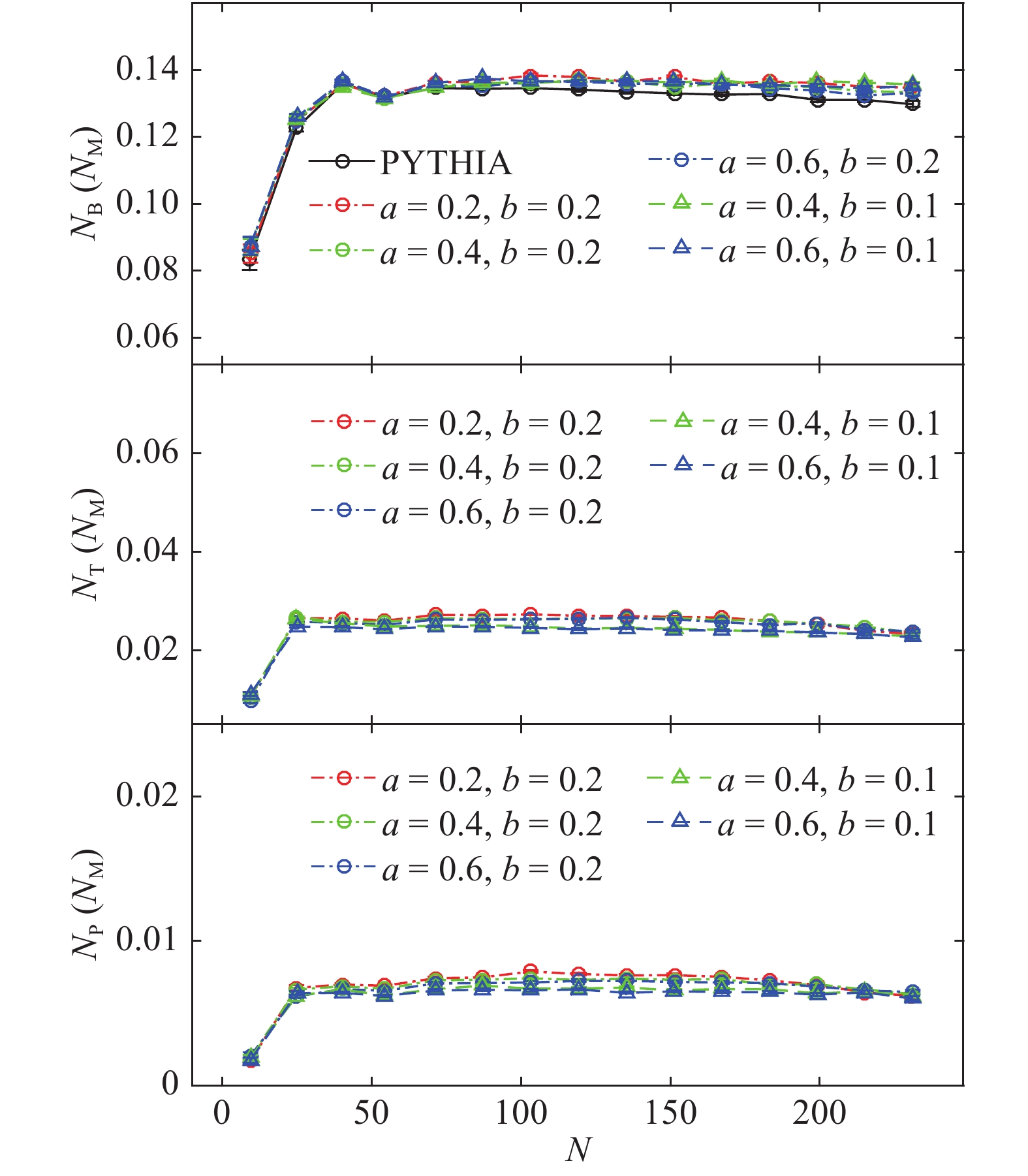Figure3. (color online) Multiplicity dependence of baryon-to-meson (top panel), tetraquark-to-meson (middle panel) and pentaquark-to-meson (bottom panel) ratios in NSD pp collisions at $ \sqrt{s}=7 \rm \ TeV $ for different combinations of interaction coefficients a and b, with fixed $ t_{f,\rm max}=4.0 \ \rm fm/c $, $ t_{f}^{'}=0.5 \ \rm fm/c $. The units of a and b (GeV/fm and $ \rm GeV \cdot fm $ , respectively) are omitted in the legends.

As shown in Fig. 2, the ratios of baryon-to-meson, tetraquark-to-meson and pentaquark-to-meson vary as functions of the total multiplicities for different combinations of $ t_{f,\rm max} $ and $ t_f^{'} $, while a and b are fixed at $ a=0.4 \ \rm GeV/fm $, $ b=0.2 \ \rm GeV \cdot fm $. From the top panel in this figure, one can see that for each distribution, R rises sharply with the increase of multiplicity for events with low multiplicity, and then changes much more slowly with the increase of multiplicity. For different combinations of $ t_{f,\rm max} $ and $ t_f^{'} $, the differences between the distributions are more obvious for events with high multiplicities ($ \langle N \rangle \gtrsim 100 $). The change of $ t_f^{'} $ has a larger effect than of $ t_{f,\rm max} $ . The increase of $ t_{f,\rm max} $ reduces the ratios for events with high multiplicity, but the ratios do not change much for events with low multiplicity ($ \langle N \rangle \lesssim 80 $). The increase of $ t_f^{'} $, by contrast, increases the ratios for high multiplicity events, but decreases the ratios for events with low multiplicity. In the middle panel, for each distribution, the tetraquark-to-meson ratio shows a sharp rise for low multiplicity events ($ \langle N \rangle \lesssim 25 $), then slowly drops with the increase of multiplicity. The ratios decrease with the increase of $ t_{f,\rm max} $ or $ t_f^{'} $ for most multiplicity intervals. The pentaquark-to-meson ratios, shown in the bottom panel, are much smaller than the other two, change little for most events with different $ t_{f,\rm max} $, and show a slight decrease with the increase of $ t_f^{'} $.
Figure 3 presents the same ratios as in Fig. 2 but for different combinations of interaction coefficients a and b, while $ t_{f,\rm max} $ and $ t_f^{'} $ are fixed, $ t_{f,\rm max}=4.0 \ {\rm fm/c} $, $ t_{f}^{'}=0.5 \ {\rm fm/c} $. As depicted in the top panel, R shows a similar tendency as in Fig. 2 for each distribution, and the differences between the distributions with different combinations of a or b are more obvious for events with high multiplicities, which resembles to the above case. For high multiplicity events ($ \langle N \rangle \gtrsim 170 $), the increase of a or b slightly decreases the ratios, but the effect of b is more obvious. For events with lower multiplicity, the change of a or b has little effect on the change of ratios. As is shown in the middle panel, the tetraquark-to-meson ratio also shows a sharp rise for low multiplicity events ($ \langle N \rangle \lesssim 25 $), then slowly drops with the increase of multiplicity for each distribution. The change of a does not have a clear effect, while the increase of b slightly increases the ratios for most high multiplicity intervals ($ \langle N \rangle \gtrsim 80 $). For the pentaquark-to-meson ratio shown in the bottom panel, there is a sharp rise for low multiplicity events ($ \langle N \rangle \lesssim 25 $), and then a slow drop with the increase of multiplicity for each distribution. The change of a does not have an evident effect. The increase of b increases the ratios slightly for most high multiplicity intervals ($ \langle N \rangle \gtrsim 80 $).
2 -->

4.2.Transverse momentum distributions

Figure 4 and Fig. 5 show the dependence of transverse momentum distributions for different values of parameters in the mid-pseudorapidity region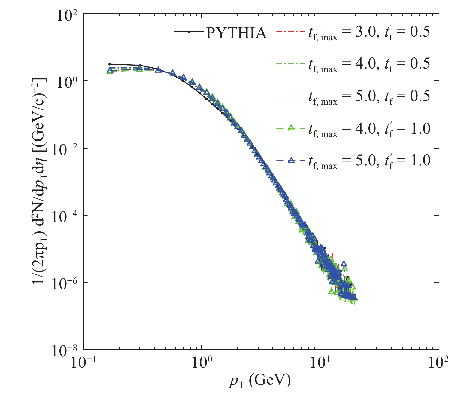 $ |\eta|<0.5 $.
Figure4. (color online) Transverse momentum distribution in the $ |\eta|<0.5 $ region in NSD pp collisions at $ \sqrt{s}=7 \rm \ TeV $ for different combinations of maximum formation time $ t_{f,\rm max} $ and time $ t_{f}^{'} $ for free flow, with fixed $ a=0.4 \ \rm GeV/fm $, $ b=0.2 \ \rm GeV \cdot fm $. The units of time (fm/c) are omitted in the legend.

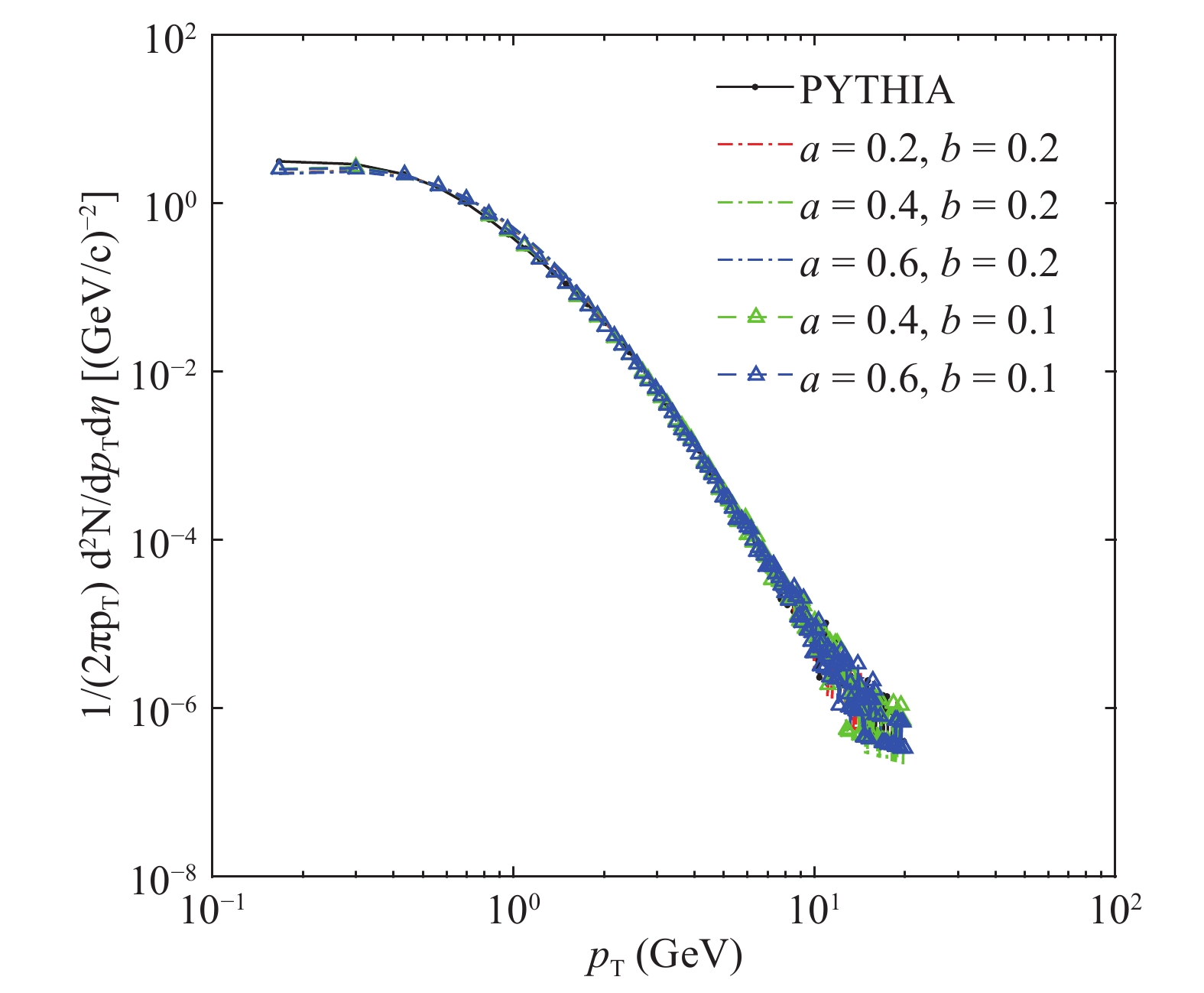Figure5. (color online) Transverse momentum distribution in the $ |\eta|<0.5 $ region in NSD pp collisions at $ \sqrt{s}=7 \rm \ TeV $ for different combinations of interaction coefficients a and b, with fixed $ t_{f,\rm max}=4.0 \ {\rm fm/c} $, $ t_{f}^{'}=0.5 \ {\rm fm/c} $. The units of a and b (GeV/fm and $ \rm GeV \cdot fm $ , respectively) are omitted in the legend.

Figure 4 presents the dependence of the transverse momentum distribution for different combinations of maximum value of formation time $ t_{f,\rm max} $ and free flow time $ t_{f}^{'} $, while a, b are fixed, $ a=0.4 \ \rm GeV/fm,\; b=$ $0.2 \ \rm GeV \cdot fm $. One can see that the transverse momentum distributions for hadrons within $ p_T\lesssim 2.0\ {\rm GeV/c}$ are clearly affected. This can be attributed to the expansion in the transverse plane such that the interactions have a more evident effect on the transverse motions of quarks. As a result, more quarks tend to get their $ p_T $ increased, which leads to a decrease of hadron number in the small $ p_T $ region and an increase in the large $ p_T $ region. With the increase of $ t_{f,\rm max} $, the deviation of the distribution from the result of PYTHIA slightly decreases. Conversely, the deviation increases with the increase of $ t_{f}^{'} $. This can be explained as follows. Since the total color of quarks from the same parent hadron is neutral, the forces acting on one quark from quarks decomposed from the same parent hadron cancel each other to a certain degree, determined by the formation time and free flow time. The increase of $ t_{f,\rm max} $ means that more quarks from different parent hadrons are separated in space, or that there is an increase of separating distances, so that the interactions between quarks from different parent hadrons weakens. The increase of $ t_{f}^{'} $ creates the opposite effect as there is a higher possibility of mixing more quarks from different parent hadrons. In other words, the values of $ t_{f,\rm max} $ and $ t_{f}^{'} $ influence the effective range of interactions. For larger $ t_{f,\rm max} $, the interactions between quarks from different parents are weaker, so that the transverse motion of quarks tends to be less affected by the other quarks during the expansion process. A larger $ t_{f}^{'} $ enhances the range of interactions, but also reduces the short-range Coulomb interactions. However, from the results one can conclude that the former is stronger, which means that a larger $ t_{f}^{'} $ will enhance the interactions and tend to increase quark $ p_T $.
The influence of different values of a and b is shown in Fig. 5. The difference between the distributions from PYTHIA and our model increases with the increase of b, while it changes little with the variation of a. Clearly b has a larger effect on the distributions, since it determines the strength of short range interaction in Eq. (1), which is much stronger than the linear part when the quarks are close to each other. This indicates that the deviation is mainly formed in the early stage of system evolution, when the quarks in the system are compact, and the Coulomb potential, as a short range interaction, is of great influence.
2 -->

4.3.Pseudorapidity distributions

Figure 6 and Fig. 7 show the pseudorapidity distributions for different values of parameters. There is no restriction on the selection of transverse momentum.
Figure6. (color online) Pseudorapidity distribution in NSD pp collisions at $ \sqrt{s}=7 \rm \ TeV $ for different combinations of maximum formation time $ t_{f,\rm max} $ and time $ t_{f}^{'} $ for free flow, with fixed $ a=0.4 \ \rm GeV/fm $, $ b=0.2 \ \rm GeV \cdot fm $. The units of time fm/c are omitted in the legend.

Figure7. (color online) Pseudorapidity distribution in NSD pp collisions at $ \sqrt{s}=7 \rm \ TeV $ for different combinations of interaction coefficients a and b, with fixed $ t_{f,\rm max}=4.0 \ {\rm fm/c} $, $ t_{f}^{'}=0.5 \ {\rm fm/c} $. The units of a and b (GeV/fm and $ \rm GeV \cdot fm $ , respectively) are omitted in the legend.

As is shown in Fig. 6, with fixed a and b, the pseudorapidity distributions are evidently different from the ones obtained with PYTHIA. The distributions in the pseudorapidity region $ |\eta|\gtrsim 2.0 $ decrease remarkably, while distributions for $ |\eta|\lesssim 2.0 $ clearly increase. Such a change can be accounted for by the increase of transverse momentum as a result of the interactions. Quarks with large pseudorapidities are often the ones with small transverse momenta or large longitudinal momenta, therefore they are very sensitive to the forces acting on them. From Fig. 1, one can see that quarks with large speeds (usually with large momenta) are often crowded in the forward-backward direction, and thus they are strongly affected by the interactions. The decrease of the maximum value of formation time $ t_{f,\rm max} $ , or the increase of free flow time $ t_{f}^{'} $ , leads to a larger deviation of the distributions from PYTHIA. The explanation for such change is the same as mentioned in Subsection 4.2 for the transverse momentum distributions. Additionally, the change of $ t_{f}^{'} $ has a larger effect on the pseudorapidity distribution than of $ t_{f,\rm max} $ .
From Fig. 7, one can see that for fixed $ t_{f,\rm max} $ and $ t_{f}^{'} $, and different combinations of a and b, the distributions deviate from PYTHIA. Similarly to the previous scenario, the distributions in the pseudorapidity region $ |\eta|\gtrsim 2.0 $ decrease remarkably, while for $ |\eta|\lesssim 2.0 $ they clearly increase. The increase of b obviously increases the deviation, while the increase of a has a much smaller effect, which indicates that the deviations from PYTHIA mainly stem from the initial stage of the evolution when the quarks are more compact.
Figure 8 and Fig. 9 show the pseudorapidity distributions of tetraquarks and pentaquarks for different combinations of parameters. One can see from these figures that the multi-quark states are mainly distributed in the very forward-backward pseudorapidity region. This can be understood from the fact that quarks in the very forward-backward pseudorapidity region have often large momenta, so that they easily stick together if they happen to be close to each other at the beginning of the evolution, and thus have a larger probability to form multi-quark states.
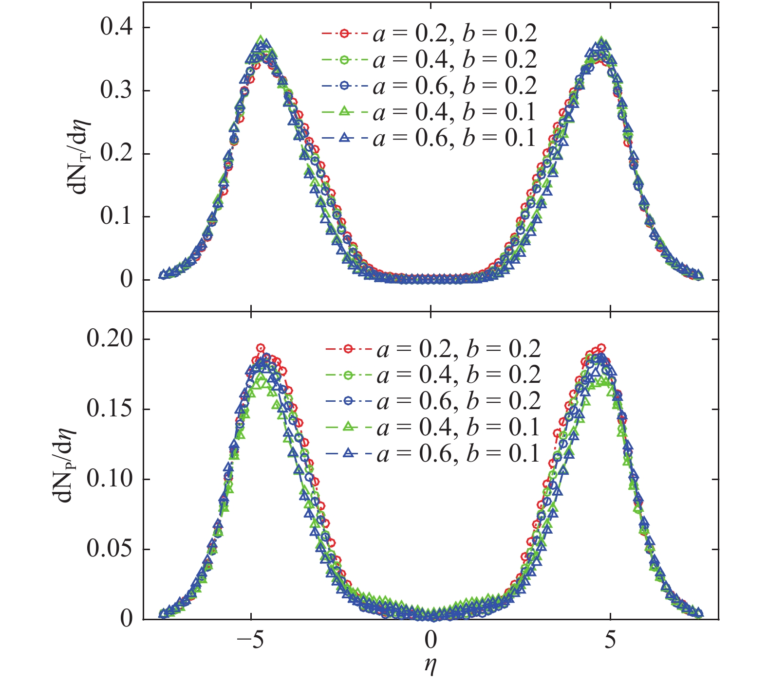Figure9. (color online) Pseudorapidity distribution of tetraquarks (top panel) and pentaquarks (bottom panel) in NSD pp collisions at $ \sqrt{s}=7 \rm \ TeV $ for different combinations of interaction coefficients a and b, with fixed maximum value of formation time $ t_{f,\rm max}=4.0 \ {\rm fm/c} $, and free flow time $ t_{f}^{'}=0.5 \ {\rm fm/c} $. The units of a and b (GeV/fm and $ \rm GeV \cdot fm $ , respectively) are omitted in the legends.

Figure8. (color online) Pseudorapidity distribution of tetraquarks (top panel) and pentaquarks (bottom panel) in NSD pp collisions at $ \sqrt{s}=7 \rm \ TeV $ for different combinations of maximum formation time $ t_{f,\rm max} $ and time $ t_{f}^{'} $ for free flow, with fixed $ a=0.4 \ \rm GeV/fm $, $ b=0.2 \ \rm GeV \cdot fm $. The units of time fm/c are omitted in the legends.

2 -->

4.4.Forward-backward multiplicity correlations

Correlations and fluctuations are important tools for studying the mechanism of particle production in high energy collisions. The correlations and fluctuations of produced particles may change significantly in a phase transition because of the change of degrees of freedom. Forward-backward multiplicity correlations have been studied widely to analyze the mechanism of particle production [47, 48] , and they played an important role in the development of mechanisms of multi-parton interactions in the PYTHIA model [49]. The forward-backward multiplicity correlations are usually defined as correlation coefficients of forward and backward multiplicities

${b_{\rm corr}} = \frac{{\langle {n_F}{n_B}\rangle - \langle {n_F}\rangle \langle {n_B}\rangle }}{{\sqrt {(\langle n_F^2\rangle - {{\langle {n_F}\rangle }^2})(\langle n_B^2\rangle - {{\langle {n_B}\rangle }^2})} }},$

(16)

where $ n_F $ and $ n_B $ are the number of particles in the forward and backward pseudorapidity intervals which are symmetrically located. For symmetric distributions (e.g. those from pp collisions), Eq. (16) can be rewritten as

${b_{\rm corr}} = \frac{{\langle {n_F}{n_B}\rangle - {{\langle {n_F}\rangle }^2}}}{{\langle n_F^2\rangle - {{\langle {n_F}\rangle }^2}}}.$

(17)

In our study, we chose the forward and backward pseudorapidity regions symmetrically with a pseudorapidity gap $ \eta_{\rm gap} $ and width $ \delta \eta $ for each side. The correlation strengths from our model are about ten percent larger than those from the original PYTHIA model, and are shown in Fig. 10 and Fig. 11 for different sets of parameters. As depicted in these figures, there is a decrease of correlation strength with the increase of pseudorapidity gap, and an increase with the increase of interval size.
Figure11. (color online) Forward-backward correlations in NSD pp collisions at $ \sqrt{s}=7 \rm \ TeV $ for different combinations of interaction coefficients a and b, with fixed $ t_{f,\rm max}^{'}=4.0 \ {\rm fm/c} $, $ t_{f}^{'}=0.5 \ {\rm fm/c} $. $ \delta \eta $ is the interval size selected symmetrically, and $ \eta_{\rm gap} $ is the variable central separation. The units of a and b (GeV/fm and $ \rm GeV \cdot fm $) are omitted in the legends.

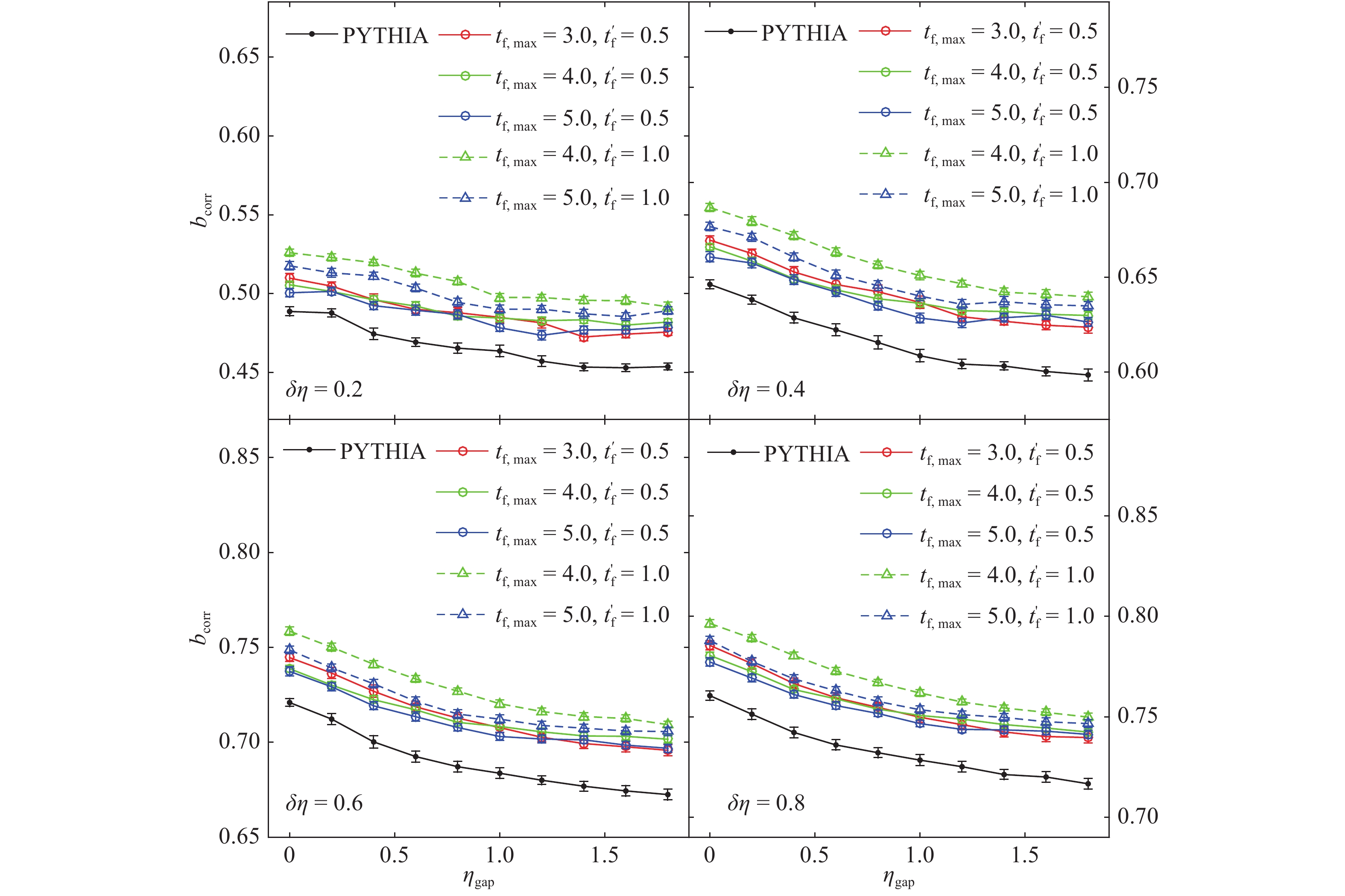Figure10. (color online) Forward-backward correlations in NSD pp collisions at $ \sqrt{s}=7 \rm \ TeV $ for different combinations of maximum formation time $ t_{f,\rm max} $ and time $ t_{f}^{'} $ for free flow, with fixed $ a=0.4 \ \rm GeV/fm $, $ b=0.2 \ \rm GeV \cdot fm $. $ \delta \eta $ is the interval size selected symmetrically, and $ \eta_{\rm gap} $ is the variable central separation. The units of time fm/c are omitted in the legends.

Figure 10 presents the dependence of forward-backward correlations as function of $ \eta_{\rm gap} $ and $ \delta \eta $ for different values of maximum formation time $ t_{f,\rm max} $ and free flow time $ t_{f}^{'} $ , with fixed $ a=0.4 \ \rm GeV/fm $, $ b=0.2 \ \rm GeV \cdot fm $. The change of $ t_{f}^{'} $ has a larger effect than of $ t_{f,\rm max} $. The increase of $ t_{f,\rm max} $ slightly decreases the correlations for different $ \delta \eta $ for most pseudorapidity gaps, whereas the increase of free flow time obviously enhances the correlations with different pseudorapidity gaps and widths. This can be explained by observing that the increase of free flow time brings quarks from different parent hadrons closer, while the increase of $ t_{f,\rm max} $ tends to weaken such mixing. This mixing enhances the correlations of final hadrons.
The dependence of the correlations on parameters a and b is presented in Fig. 11. The increase of b leads to an increase of correlations, whereas the change of a has little effect, which indicates that the contribution to correlations is mainly from the initial interactions, when the partons are close and the Coulomb term in Eq. (1) plays a major role in the evolution process.

In this paper, a hadronization mechanism based on color interactions among relativistic quarks was discussed and applied to a study of hadronization in high energy pp collisions. The distributions and forward-backward correlation strengths from simulations with different parameters were compared to PYTHIA. Our study focused on the effects of the dynamics, controlled by several parameters, on the final distributions and correlations. The initial geometry was determined according to a method inspired from the AMPT model, while the interacting potential is of the Cornell type. The effects of color interactions, maximum formation time and free flow time were discussed. As revealed by the results, the free flow time and the Coulomb interaction have considerable effects on all hadron distributions and correlations.
The present work could be improved in several aspects:
(1) The initial space positions of hadrons and quarks should stem from a more solid basis;
(2) The form of interaction should include more realistic physical effects, such as Debye screening etc.;
(3) Relativistic retarding effect could also be considered. All of these will be considered in a future work.