HTML
--> --> -->The analysis of fronts has always been an important task in weather forecasting. To date, frontal analysis in operational forecasting generally depends on manual analysis, which considers various factors, such as temperature, humidity, wind direction, and sea level pressure. However, it is worth noting that manual analysis of the frontal line is usually time-consuming and subjective (McCann et al., 2001). Therefore, many researchers have proposed objective identification methods for fronts. The pioneering work of Renard and Clarke (1965) proposed the thermal frontal parameter (TFP) based on grid data to identify and locate fronts. Based on Renard and Clarke (1965), Hewson (1998) proposed the classic thermodynamic front identification method (Hewson, 1998, hereinafter referred to as H98). In H98 the potential locations of fronts are first drawn according to the

Simmonds et al. (2012) used the direction and velocity changes of the 10 m wind to determine the frontal position (known as the wind method) and pointed out that the number of fronts, mean frontal length, and frontal intensity have different seasonal characteristics between 30°–50°S and 50°–70°S. Schemm et al. (2015) compared the frontal activities in the Northern Hemisphere identified by the wind method and the thermal method and showed that the thermal method has a good ability to identify fronts with strong baroclinicity, while the wind method is better suited for the identification of meridionally oriented moving fronts. Parfitt et al. (2017) proposed a new objective identification method for fronts, called the F diagnostic, which adopted the horizontal temperature gradient and relative vorticity to identify fronts. Lagerquist et al. (2020) used a convolutional neural network method to detect fronts over North America and found a significant influence of El Ni?o on winter fronts. To supplement the research on the horizontal structure of fronts, Kern et al. (2019) recently proposed a visualization approach to analyze the three-dimensional structure of atmospheric fronts and their related physical and dynamical processes.
Since the mid-2000s, extreme cold events have occurred more frequently than during the 1990s and early 2000s when the East Asian winter monsoon tended to be weak (Cohen et al., 2014; Wang and Chen, 2014; Lu et al., 2016; Wu, 2017; Ma et al., 2018). Cold frontal activities are frequent during the Eurasian winter, and cold fronts with strong cold air activities may cause major disastrous weather events. Previous studies on the long-term activity of hemispheric-scale frontal surfaces have mainly focused on the extratropical storm tracks in the North Atlantic and the North Pacific, where atmospheric baroclinicity is strong and frontal features are more obvious. However, to date, no specific research has been conducted on the activity of wintertime cold fronts in Eurasia. Therefore, this study proposed a two-step cold front identification method using the TFP criteria and temperature advection based on high-resolution data. Moreover, the applicability of this method was verified for wintertime in Eurasia.
2.1. Data
The ERA-5 reanalysis data from the European Centre for Medium-Range Weather Forecast model (ECMWF) with a spatiotemporal resolution of 0.25° × 0.25° and one hour are used in this paper, including temperature and wind components at 850 hPa, surface wind components, and sea level pressure (SLP) from 1989 to 2019 (Hersbach et al., 2020). We also adopt the daily dataset with basic meteorological elements from the national ground weather stations in China (V3.0) (2
2.2. Methods
32.2.1. Two-step cold front identification method
A front can be essentially understood as an interface between warm and cold air masses, which is a three-dimensional inclined surface. Its intersection with a certain isobaric surface is a dense isotherm zone, called the frontal zone. The warm boundary of the frontal zone on the isobaric surface (such as 850 hPa) in the lower troposphere can represent the location of the surface cold front. The TFP proposed by Renard and Clarke (1965) is widely used to locate the front.where τ can be any suitable thermodynamic variable. The thermal parameter in this paper is the temperature (T) at 850 hPa, and it is smoothened 100 times with a five-point smoothing technique. In the previous objective identification of a front, the TFP was used directly to locate the front. For example, Berry et al. (2011b) used the frontal location equation


3
2.2.1.1. Identification of the cold frontal zone
To determine the cold frontal zone, the high-resolution ERA-5 reanalysis data are used to calculate the TFP and the temperature advection (


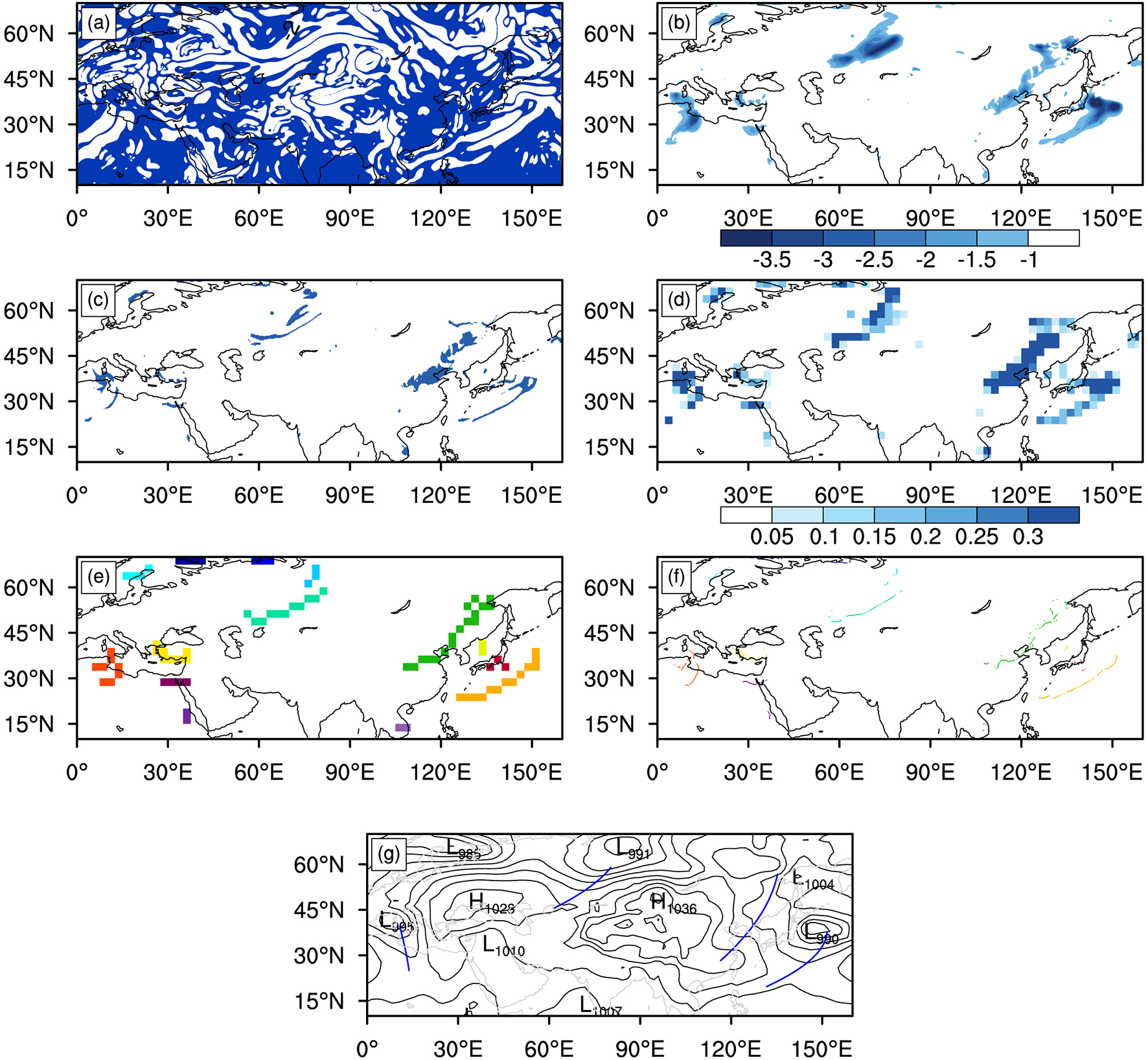 Figure1. An example of front detection at 1200 UTC on 28 November 2008. (a)

3
2.2.1.2. Cold front identification
After delineating the frontal zone, we need to determine the warm boundaries of the frontal zone to draw the front. The grid points on the eastern and southern boundaries of each identified cold frontal zone in Fig. 1d are retained, and each boundary is plotted in a different color (Fig. 1e). Then, the high-resolution (0.25° × 0.25°) frontal grids within the boundaries at the low resolution (2.5° × 2.5°) are shown in Fig. 1f. It can be seen that these sets of featured grids are distributed like a curve in different colors and indicate different potential cold fronts. Finally, a second-order polynomial fitting is applied to the marked frontal grids in the same color, and each smoothed curve indicates a cold front identified with the objective method. The cold fronts with lengths less than 800 km are deleted. As shown in Fig. 1g, the objectively identified cold fronts are well organized, and the result reveals four cold fronts located in the southern Mediterranean Sea, the eastern Caspian Sea, and along the coast of East Asia at 1200 UTC on 28 November 2008.3
2.2.1.3. Thresholds of cold front parameters
To investigate the sensitivity of different thermodynamic parameters and their thresholds, we documented a case at different thresholds of temperature advection or TFP as well as different parameters for TFP in the same cold detection case in Fig. 1 (Fig. 2). More “frontal” grids are detected as the threshold of temperature advection becomes less negative (Fig. 2b), but most of them are just noise for the cold front detection without a clear frontal structure. On the other hand, the increase in the threshold of TFP results in a decrease in the number of frontal grids and leads to a discontinuous and blurry frontal zone (Fig. 2c), which is unfavorable for cold front detection. Other thermal parameters such as potential temperature (θ), equivalent potential temperature (θe), and pseudo-equivalent potential temperature (θse) at 850 hPa are also selected for the TFP calculation. All the four cold fronts in the above case are consistently displayed in Figs. 2d–2f, indicating that the identification of different thermal parameters is similar. For simplicity, the temperature at 850 hPa is used for the TFP calculation below. Figure2. The selected cold frontal zones (shading) with different TFP parameters and different thresholds of temperature advection and TFP at 1200 UTC on 28 November 2008. (a)


3
2.2.2. Subjective analysis of cold fronts
The subjective analysis (SA) for cold fronts based on temperature, wind field, temperature advection at 850 hPa, as well as the SLP and surface wind field (10 m) is also conducted (Fig. 3). The cold frontal zones at 850 hPa are marked as the areas with strong horizontal temperature gradients accompanied by strong cold advection (Fig. 3a). Accordingly, a cold front is subjectively analyzed as the consecutive line of the local maximum of surface horizontal wind shear over the above-mentioned frontal zone, which usually is co-located within the region of influence of an extratropical cyclone or along the frontier of a surface cold high. Correspondingly, the cold fronts in the same case as shown in Fig. 1 can be obtained, which are indicated by the green lines in Fig. 3b. Figure3. The subjective analysis of cold fronts at 1200 UTC on 28 November 2008. (a) The distributions of isotherm (red lines, interval of 4 K), temperature advection (shading, interval of 0.5 × 10?4 K s?1), and horizontal wind field (arrows) at 850 hPa. (b) The subjective-analysis cold fronts (green lines), the SLP (contours, hPa), and the surface horizontal wind field (arrows).
3.1. Comparison of three identification methods
In order to evaluate the reliability of our objective method, the tracks of the cold front from 0000 UTC 27 February 27 to 0000 UTC 2 March 2017, are detected by our objective method, a traditional thermodynamic method, and the SA method (Fig. 4a). The calculation of the traditional thermodynamic method refers to Berry et al. (2011b). The consistent movement of the cold front from Lake Baikal to the coast of East Asia is identified by all three methods. The cold fronts were generated on the southeastern edge of the cold high, and the surface air temperature decreases correspondingly at the posterior areas of the cold front (Figs. 4b–4e). The split of the cold front on 2 March 2017, is captured by all three methods. Its southern part moved fast into the Northwest Pacific, while the northern part is still near Vladivostok (43°08′N, 131°54′E). Comparatively, the location of the cold front identified with our method is more consistent with the result of SA than that of the traditional thermal identification method. In particular, the southern part of the cold front is missed during the last two time steps in the traditional thermodynamic method, and the direction of the cold front is even tilted to that in the other two methods. Therefore, our objective method offers a better description of this cold front event.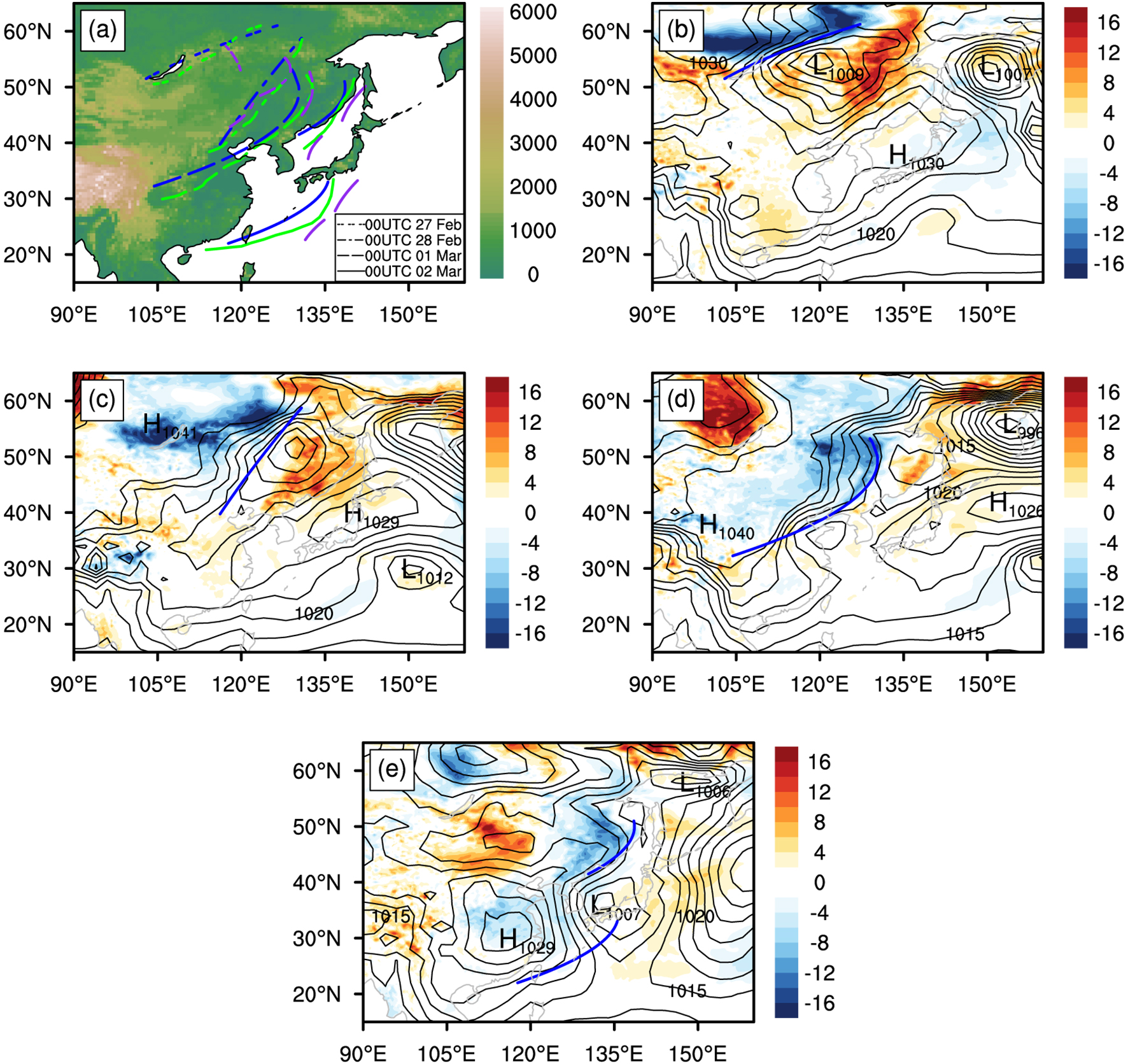 Figure4. (a) The movement of a cold front in East Asia from 27 February to 2 March 2017. The blue lines represent the auto-identified cold fronts, the green lines represent the subjective-analysis cold fronts, and the purple lines represent the cold fronts from traditional thermal identification and the terrain height (shading, m). The short-dotted lines, the dotted lines, the long-dotted lines, and the solid lines denote 27 February, 28 February, 1 March, and 2 March, respectively. The SLP (black contours, hPa), the 24-hourly variation of T2m [shading, °C (24 h)?1] and the auto-identified cold front (blue line) at (b) 0000 UTC 27 February, (c) 0000 UTC 28 February, (d) 0000 UTC 1 March and (e) 0000 UTC 2 March 2017.
2
3.2. An extreme precipitation case associated with a cold front
During the period from 0000 UTC on 7 November to 0000 UTC on 8 November 2016, a regional extreme precipitation event associated with a cold front occurred in southern China. The 24-hour accumulated precipitation in Jingjiang, Zhongxian, and Pengshui on 7 November reached 58.0 mm, 61.4 mm, and 59.9 mm, respectively. The cold front moved southeastward with a speed of nearly 25 km h?1, and it split and remerged in the last two time steps (Fig. 5a). It can be seen that the cold front in this event was located on the edge of the strong cold high. The direction of the cold front was parallel to the southeast border of the cold high, and the areas with heavy rainfall are mainly behind the cold front (Fig. 5b–5d). According to the distributions of SLP and precipitation, our objective identification method can reasonably describe the cold front in the heavy rainfall event.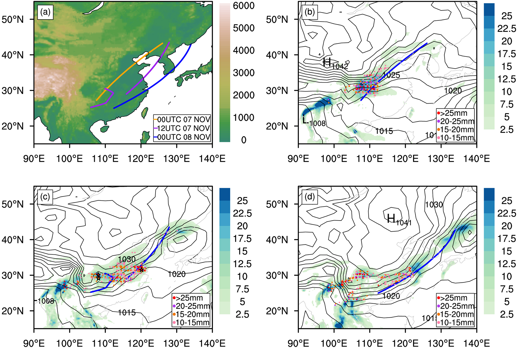 Figure5. (a) The auto-identified cold fronts at 0000 UTC (orange line), 1200 UTC (purple line) on 7 November, and 0000 UTC (blue line) on 8 November 2016, and the terrain height(shading, m). The SLP (black contours, hPa), the 12-hour accumulated precipitation based on the reanalysis [shading, mm (12 h?1)] and observational data [colored dots, units: mm (12 h)?1] and the auto-identified cold front (blue line) at (b) 0000 UTC, (c) 1200 UTC 7 November 2016, and at (d) 0000 UTC 8 November 2016. The black star markers indicate the weather stations of Jingjiang (31.59°N, 120.16°E), Zhongxian (30.18°N, 108.02°E) and Pengshui (29.18°N, 108.1°E) in China.
2
3.3. Objectively identified cold fronts in a continuous period
To further evaluate the reliability of our algorithm, a multi-cold front case in East Asia during a continuous period is shown in Fig. 6. At 1200 UTC on 3 December 2009, there were two cold fronts in East Asia, with one on the edge of the surface high near Lake Baikal and the other on the edge of the surface high over the East Asian coast. The cold front near Lake Baikal moved southeastward and gradually entered the cyclone in front of the surface high from 1200 UTC on 3 December to 0000 UTC on 6 December. The cold front along the East Asian coast moved eastward into the cyclone on the ocean and left the study area at 0000 UTC on 5 December. A cold front appeared in the cyclone in Siberia at 1200 UTC on 4 December, and it moved southeastward and disappeared at 1200 UTC on 5 December. In short, the direction and moving speed of the cold front show good consistency with the surface high-low pressure systems, which indicates a good performance for our method to identify multiple cold fronts over a large area. Figure6. The auto-identified cold fronts (blue lines) and the SLP (contours, hPa) from 1200 UTC 3 December to 0000 UTC 6 December 2009 (interval of 12 hours).
2
3.4. Application on the cold air activities in Eurasia
A nationwide disastrous cold air outbreak in China ensued from 22 December to 26 December 2009. The temperature in northern China sharply dropped by 10°C–25°C within 24–48 hours, accompanied by severe weather events, such as a blizzard and sandstorm in northwestern China, which brought great losses to local societies. In fact, this event resulted from the invasion of a strong surface cold high and can also be indicative of a cold front activity. Figure 7 shows the movement of the auto-identified cold front and the associated cooling from 1200 UTC 22 December to 1200 UTC 25 December 2009. In particular, a strong cold high originating from western Siberia moved eastward and notably extended southeastward, which strengthened after reaching the Mongolian Plateau. Consistently, a cold-high-associated front was detected, which passed through the Sayan Mountains, Lake Baikal, Mongolia, the North China Plain, and the East Asian coast. Correspondingly, strong cold advection appeared behind the cold front with the maximum 24-hour temperature decrease reaching above 16 °C (Figs. 7 and 8).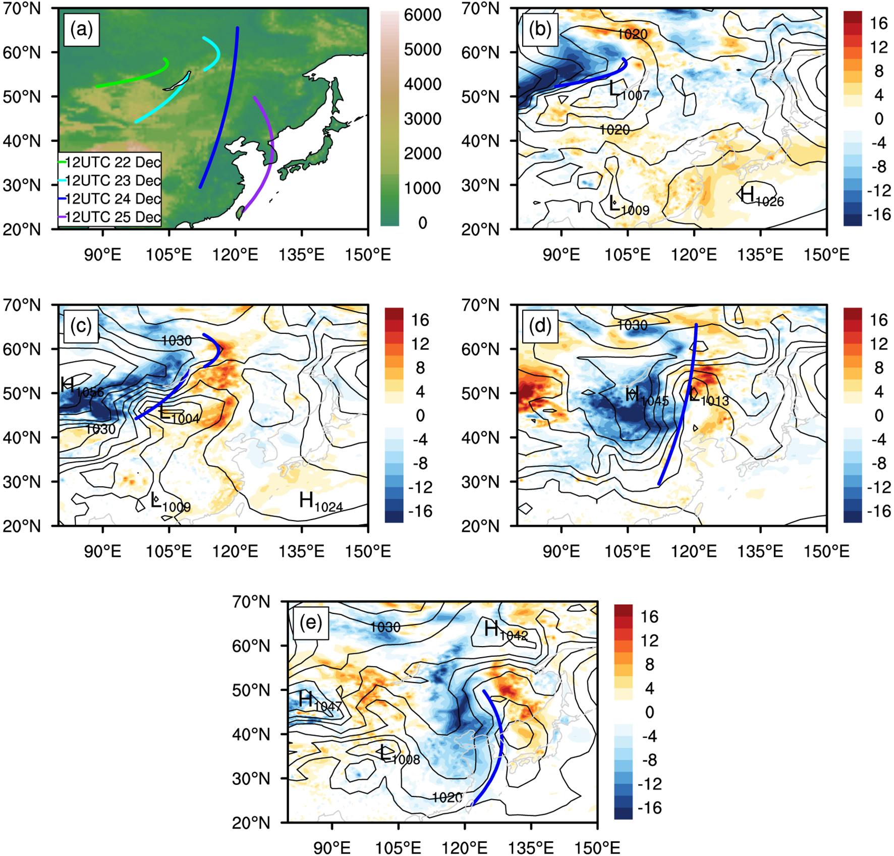 Figure7. (a) The auto-identified cold fronts from 1200 UTC 22 December to 1200 UTC 25 December 2009 (interval of 24 hours), and the terrain height (shading, m). (b–e) The SLP (black contours, hPa), the 24-hourly variation of surface air temperature based on the reanalysis data [shading, °C (24 h)?1] and the auto-identified cold front (blue line) from 1200 UTC 22 December to 1200 UTC 25 December 2009 (interval of 24 hours).
 Figure8. The large-scale atmospheric circulation from 1200 UTC 22 December to 1200 UTC 25 December 2009 (interval of 24 hours). The temperature (red contours, K) and the geopotential height (black contours, dagpm) (a, c, e, g) at 500 hPa and (b, d, f, h) 850 hPa and the horizontal wind field (arrows) at 850 hPa.
The geopotential height and temperature fields at 500 hPa and 850 hPa in this cold wave event are also shown (Fig. 8). There was a well-developed ridge over the Urals at 500 hPa, accompanied by a wide trough in front of it over western Siberia. Correspondingly, a significant horizontal pressure gradient at 500 hPa (Fig. 8a) and an associated frontal zone (Fig. 8b) appeared near the Sayan Mountains. The cold front was located on the warm side of the 850 hPa frontal zone at this moment (Fig. 8b). On 23 December, the middle-high latitude circulation over the Eurasian sector became more meridional, and the 500 hPa trough moved to the Mongolian Plateau from western Siberia. Behind the trough, a temperature ridge was slightly ahead of the geopotential height ridge (Fig. 8c), which can weaken the baroclinic wave near western Siberia, and facilitated the eastward movement of the 850 hPa frontal zone (Fig. 8d). On 24 December, the 500 hPa trough moved eastward rapidly (25° d?1), and the northwesterly wind behind the trough induced the southward movement of the cold air from high latitudes (Fig. 8e). The 850 hPa frontal zone also moved southward rapidly (Fig. 8f) as the cold front advanced into Mongolia and the North China Plain. A pronounced cold air outbreak occurred during the period from 23–24 December, and thus northwestern China suffered from disastrous cold weather. On 25 December, the 500 hPa trough continued to move eastward (Fig. 8g), and the 850 hPa frontal zone further advanced southward (Fig. 8h). The cold front then proceeded southeastward, affecting Northeast China and the Jianghuai region.
In addition, the temperature change behind the front could be affected by the topography. Figure 7b shows that a cold front was located in the northern edge of the Sayan Mountains, and the plain was behind the cold front, with severe cooling. However, once the cold front climbed up to the Mongolian Plateau, the decreased temperature right behind the cold front was weak, and the temperature even slightly increased in some areas (Fig. 7c). Because the altitude of the Mongolian Plateau is high with comparative low temperature, the cooling effect behind the cold front is not pronounced when a cold front passes by this region.
In this cold wave event, the auto-identified cold fronts correspond well with the circulation systems in the middle and lower troposphere. In particular, the cold wave broke out rapidly from 23–24 December, and the sudden acceleration of the cold front was well captured by our method.
2
3.5. Frequency of cold fronts
The two-step cold front identification method that is applied over Eurasia in wintertime covers September to March over the 30-year period from 1989 to 2018 by using the ERA-5 dataset. Figure 9 shows the mean frequency (expressed as a percentage of time) of cold frontal occurrence in wintertime, noting that locations near the Tibet Plateau are masked out. The cold fronts frequently appear in the Baltic Sea, the Mediterranean, Africa, and the east of the Ural Mountains, with frequencies greater than 4%. The frequency of cold fronts along the coast of East Asia has a maximum value of 20%. On the coast of East Asia, the frequency of cold fronts is the maximum observed over the three regions, including North China, the Sea of Japan, and the coast of Japan.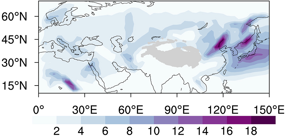 Figure9. The mean frequency (expressed as a percentage of time) of cold fronts during the wintertimes of 1989–2018.
In addition, the method and the obtained front dataset may be utilized to comprehensively investigate the extratropical weather systems and their associations with the front. For example, there are distinct interactions between fronts and topography (Hewson, 2001). Large mountains such as the Alps (Jenkner et al., 2010) and the Brazilian Plateau (Foss et al., 2017) can block dry and cold postfrontal air masses and slow down the cold front on the windward side. It can also be seen from Fig. 9 that the places which have higher frequencies of cold fronts in Eurasia are mostly located on the east or southeast side of high terrain. Therefore, the topographic effects of large mountains over the Eurasian continent on the cold frontal activities, such as the changes in their intensity, movement, and vertical structures deserve further investigation. Meanwhile, the increasing low-temperature extremes in mid-latitude Eurasia alongside the recent Arctic amplification (e.g. Cohen et al., 2014) have been of increasing interest. The potential for detecting and tracking mid-latitude cold fronts using this algorithm presented in this study may shed light on the study of the mid-latitude Eurasian climate.
Acknowledgements. The authors express their appreciation for the staff at the China Meteorological Data Service Centre and ECMWF for providing the freely available datasets. This work is supported by the National Key Research and Development Program of China under contract (Grant No. 2019YFC1510201 and Grant No. 2018YFC1505602). We hereby give thanks to the reviewers for their very constructive and useful comments.
Summary and Comparison between Two Methods
The warm boundary of a frontal zone is usually regarded as a cold front. As proposed by Hewson (1998) and followed by Berry et al. (2011b), the warm boundary of a frontal zone is expressed as the contour line with a value of


 FigureA1. A sketch of the two algorithms.