HTML
--> --> -->In the global NWP models, the use of geostationary satellite observations is well demonstrated. For example, based on the four dimensional variational (4DVar) system, the European Centre for Medium-Range Weather Forecasts (ECMWF) assimilates Meteosat visible and infrared imager (MVIRI) onboard Meteosat-7 (K?pken et al., 2004) and the Spinning Enhanced Visible and InfraRed Imager (SEVIRI) on board Meteosat-8 (Schmetz et al., 2002). In the National Centers for Environmental Prediction (NCEP) global data assimilation system, the GOES imager observations are assimilated using three dimensional variational assimilation (3DVar). For regional NWP models, Stengel et al. (2009) explored the impact of SEVIRI assimilation with the 3DVar system (10 km) and 4DVar system (22 km) with the France/Aldin model respectively. Zou et al. (2011) and Qin et al. (2013) assimilated GOES imager with the NCEP Gridpoint Statistical Interpolation (GSI) 3DVar scheme using 9 and 10 km resolutions, respectively, for improving the track and intensity forecast for Hurricane Debby (2012) as well as the precipitation skills over the coastal areas of the Gulf of Mexico. Wang et al. (2018a) assimilated the layer precipitable water (LWP) retrieved from the Advanced Himawari-8 imager (AHI) for local storms. The impact of the cumulus parameterization schemes on assimilating the AHI LWP data are also studied in Lu et al. (2019). In the Weather Research and Forecasting Data Assimilation (WRFDA) system (Barker et al., 2012), Yang et al. (2017a) assimilated GOES imager radiances for convection-permitting (4 km) forecasts over Mexico. Wang et al. (2018b) investigated the added value of clear-sky AHI radiances assimilation on the analyses and forecasts for a severe storm using the WRFDA.
The above studies prove that NWP can be improved by assimilating the Infrared (IR) Radiances data from geostationary satellites measurements that are sensitive to the mass and thermal state, such as temperature, pressure and wind. However, less appreciated is the benefit of satellite data measuring atmospheric moisture, clouds and precipitation (Geer et al., 2017, 2019), since it is not possible to improve the model initial conditions by holding cloud constant in DA. It is also very desirable to fully utilize the cloud information from the IR channels, since the cloud development is observed earlier by the IR channels than precipitation by the radar observations. Thus, the problem of under-utilizing humidity and precipitation information from IR channels needs to be addressed (Chevallier et al., 2001; Chevallier and Kelly, 2002) through all-sky IR radiance assimilation. Because of the uncertainties and complexities of the cloudy radiance simulation in the radiative transfer models and the analysis techniques with clouds considered, the all-sky assimilation of IR channels is among one of the most challenging issues in DA (Li et al., 2016b). Generally, the difficulties exist in the zero-gradient problems for the clear background, the complex statistics of the situation dependent background error, the observation errors and the simulation accuracy in the radiative transfer models. Recently, Minamide and Zhang (2017) investigated an adaptive observation error inflation method to limit the erroneous analysis increments due to large representativeness errors, as is often the case for cloud-affected radiances for GOES-16. Harnisch et al. (2016) investigated a unified method to assimilate the two humidity channels at 6.2 and 7.3 μm from Meteosat Second Generation (MSG) considering the nonlinear impact of clouds on both observation and model forecast as well as the systematic deficiency of model and observation operator. Based on a local ensemble transform Kalman filter (LETKF, Hunt et al., 2007) method, Okamoto (2017) evaluated the all-sky Himawari-8/AHI IR radiance assimilation in a mesoscale NWP model with 5-km resolution using LETKF after studying the observation error models. Okamoto et al. (2019) further compared the assimilation clear-sky and all-sky IR radiances for Himawari-8/AHI in a mesoscale system using a single humidity band. Improvements for temperature, water vapor, wind, and rainfall are found in their study because of the universal coverage of Himawari-8/AHI. They also proposed adaptive bias correction schemes by setting different predictors for all-sky IR radiance assimilation. Similar studies include that of Sawada et al. (2019), who assimilated Himawari-8/AHI radiances every 10-minutes to improve convective predictability. Zhang et al. (2018) assimilated all-sky IR radiances from GOES-16 ABI using EnKF for 1 km model convection-permitting severe thunderstorms prediction for a tornado case with an adaptive observation and first guess error inflation methods. They found that by removing spurious clouds, good estimation of ice particle and liquid particle fields could be analyzed. Honda et al. (2018a) conducted Himawari-8/AHI radiances assimilation every 10 minutes to improve convective predictability. The assimilation of all-sky Himawari-8 AHI radiance for the moisture and hydrometeor initialization for TC predictions were also studied with promising results (e.g., Honda et al., 2018b, 2019; Minamide and Zhang, 2018).
This study aims to evaluate the effects of assimilating the clear-sky and all-sky IR radiances from Himawari-8 for a severe storm over north China in the framework of WRFDA using the 3DVar. The differences between the clear-sky and all-sky AHI radiance DA analyses and forecasts are explored to provide some guidelines for the usage of AHI radiance data with high spatial and temporal resolutions.
This paper is organized as follows. The introduction of the WRFDA-3DVar system, the AHI IR radiance assimilation methods, and the background error modeling method are provided in section 2. Section 3 describes the experiment design and DA configurations. The results are illustrated in Section 4 before concluding in section 5.
2.1. 3DVar method in WRFDA
The cost function is the core of the 3DVar data assimilation technique. For the traditional 3DVar method of the WRFDA (Barker et al., 2012), the prescribed cost function is designed to achieve the optimal analysis through minimization iteratively as:where

2
2.2. AHI radiance Observation Operator, Quality Control and Cloud Detection
The Community Radiative Transfer Model (CRTM: Liu and Weng, 2006) is the forward operator applied in our DA experiments. CRTM is enabled to simulate both the clear-sky and all-sky radiance. The temperature and moisture profiles from the model are the essential inputs for the clear-sky radiance simulation, while extra hydrometeor inputs (such as the cloud rainwater mixing ratio) are also needed for the all-sky radiance simulation. To conduct satellite DA, the corresponding tangent linear model and adjoint model are required in addition to the forward operator. CRTM has proven to be quite efficient with the Jacobian model included for calculating the Jacobians.As is well known, it is necessary to correct the systematic biases before DA (Dee and Uppala, 2009) by modifying the observation operator with the bias considered (Liu et al., 2012; Xu et al., 2013; Otkin et al., 2018). The modification includes four potentially state-dependent predictors (200–50 hPa, 1000–300 hPa layer thicknesses, surface skin temperature, and total column water vapor) along with their coefficients, as well as a constant component of total bias. The variational bias correction [VarBC: (Auligné et al., 2007)] scheme is employed in this study. The bias information for the water vapor channels is estimated based upon the departure (observation minus simulated clear-sky radiance from the model background) information of the two week-long period from 0000 UTC 25 June 2018 to 0000 UTC 9 July 2018. Then, the bias correction is performed with VarBC, so that the correction coefficients of the predictors are updated along with the variational analysis during the minimization procedure. As is known, the OMB (observation minus background) errors under the all-sky condition are from multiple unconfirmed sources (Sawada et al., 2019). It is rather complicated to consider and classify the error sources specifically for all sky pixels. Thus, the bias correction coefficients applied for the all-sky AHI IR radiance assimilation in this study are only estimated based on the clear sky pixels excluding the cloud sky pixels. Therefore, it is reliable to directly ingest the bias correction coefficients under clear-sky conditions to represent those under all-sky conditions.
For the all-sky AHI IR radiance DA in our current study, no quality control procedure is conducted, since the situation-dependent observation error model is applied. It should be pointed out that the observation error model may not be able to include all the error sources from the observations. Nevertheless, it is of interest to validate the observation error model by considering all kinds of observations without any quality control procedure. For the clear-sky AHI IR radiance DA, strict quality control procedures are required since the retention of erroneous AHI IR radiance data after quality control is likely to ruin the analyses. Erroneous data after quality control tend to further affect the design of the bias correction procedures. Clear-sky AHI IR radiance DA uses a range of quality controls, including:
(1) removing pixels where satellite zenith angels are larger than 65°;
(2) removing pixels where channels are over mixed surface types;
(3) removing pixels where the standard deviation of the neighboring 9 observation points for channel 13 (10.4 μm) is larger than 2 K;
(4) removing pixels with a gross check, namely |OMB| ≥8 K;
(5) eliminating data if bias-corrected innovation is larger than 3 times the observation error under clear-sky conditions. The clear sky observation errors will be described in section 2.3;
(6) eliminating cloudy pixels with the cloud detection schemes that will be introduced as below.
Clear-sky AHI IR radiance data assimilation relies on a cloud detection technique to separate the cloudy AHI IR radiances from the clear-sky AHI IR radiance before assimilation, allowing a better use of available data. The cloud-detection algorithm (named ZZ-cloud detection scheme hereafter) developed by Zhuge and Zou (2016) are applied to search different cloud cases to achieve a composite cloud mask (Wu et al., 2020). In this study, the ZZ-cloud detection scheme is enhanced in the framework of WRFDA system initially. With the 10 tests in the ZZ-cloud detection algorithm, the metrics provided by different tests indicate the signals for discriminating the existence of the cloud.
2
2.3. AHI Radiance Observation Error Model
Among the key issues of the all-sky AHI IR radiance data assimilation technology, the correct estimation of the observation errors has an important impact on the quality of the analysis because the observation error directly affects the determination of the weights for the observations in the analysis procedure. The observation errors should be assigned as situation-dependent, considering the representativeness errors that are smaller in clear-sky conditions and larger in the presence of clouds and precipitation (Geer and Bauer, 2011). The observation errors should also be channel dependent since the detection characteristics and the extent of their sensitivities to various cloud and precipitation conditions are different. Based on the observation error model in Harnisch et al. (2016), the observation error related statistics are obtained by calculating the OMB difference from 0000 UTC 4 July 2018 to 1800 UTC 7 July 2018 every 6 hours by using the 3 h forecast as the background. The brightness temperature differences of the clear-sky and the all-sky AHI IR radiance simulated with the CRTM are first calculated from the background. The differences are then binned according to the brightness temperature simulated from the background under the all-sky condition. The clear-sky AHI IR radiance simulation from CRTM needs to remove all hydrometeors while keeping temperature and moisture profiles unchanged. The corresponding brightness temperature value is determined as the brightness temperature threshold (BTlim) of each channel, when the brightness temperature difference is less than a certain value (0.1 K). Once the BTlim of the three water vapor channels are determined, the averaged cloud amount Ca can be estimated based on both the background and the observation, indicated as:Here Obs is AHI IR radiance observation and Bak is the simulated all-sky AHI IR radiance from the background. Cxb and Cy are determined from the background and the observation respectively. The parallel relationships between the observation errors and the cloud amount are estimated based on a large amount of OMB samples (observation minus the simulated all-sky AHI IR radiance from the background). The four parameters – the minimum observation errors (SDmin), the maximum observation errors (SDmax), the minimum cloud amount Ca1, and the maximum cloud amount Ca2 – are determined from the statistics. With the four determined parameters, it is convenient to estimate the cloud amount dependent observation errors for any given Ca as follows,
2
2.4. Modeling in WRFDA-3DVar
The climatological background error statistics are computed offline with the commonly used National Meteorological Center (NMC) method (Parrish and Derber, 1992). A number of 24 h and 12 h forecasts are launched at different times over roughly one month in July of the previous year in 2017 (Chen et al., 2018). Pairs of forecasts valid at the same time with different forecast lead times are extracted by the NMC method to represent the difference through averaging them over the time and domain, for example with 24 h and 12 h forecasts, respectively. Both 24 h and 12 h forecasts contain errors, while the truth is never known. Further, the B matrix is decomposed as B=UUT with the preconditioning transform applied as Uv=x?xb (Barker et al., 2004). Here x and xb is the analysis and background respectively, while v represents the control variable.The Control Variable option 7 (CV7) is applied in this study to include the zonal wind component, the meridional wind component, the full temperature, the full surface pressure, and the pseudo-relative humidity as the control variables (Chen et al., 2016; Li et al., 2016a; Sun et al., 2016; Shen et al., 2019). In addition to the five commonly used control variables, another five hydrometeor-related control variables (snow: qs, rainwater: qr, cloud liquid: qc, ice: qi, and graupel: qg mixing ratio) are also considered using GEN_BE v2.0 software developed by Descombes et al. (2014). These hydrometeor related control variables represent the microphysical variables for both ice and liquid particles in the cost function so as to effectively assimilate the cloudy AHI IR radiance observations.
3.1. AHI observation
On 17 October 2014, the Meteorological Satellite Center of Japan Meteorological Agency launched the Himawari-8 satellite successfully into geosynchronous orbit. The AHI instrument onboard Himawari-8 has an observing capability significantly improved compared with its predecessor Himawari-7 series satellites, and is similar to the Advanced Baseline Imager (ABI) onboard U.S. GOES-R satellites in terms of the hardware configurations (Schmit et al., 2005, 2017). Full-disk imagery is provided every 10 minutes by AHI, covering Japan and China. There are 16 channels including IR channels (nadir resolution 2 km) and near-IR and visible channels (nadir resolution 0.5 or 1 km). Among them, channel 7 to channel 16 are IR channels with central wavelengths ranging from 3.9 μm to 13.3 μm. The specifications of the channel information appear in Bessho et al. (2016). In this study, the three water vapor channels of AHI IR radiance are assimilated, which are sensitive to middle-to-upper tropospheric humidity and less so to the lower troposphere moisture. The three water vapor channels include channel 8 (6.2 μm), channel 9 (6.9 μm), and channel 10 (7.3 μm). For clear-sky IR radiance assimilation, these three channels are applied in Wang et al. (2018b), For all-sky AHI IR radiance assimilation, only one humidity channel is assimilated in Minamide and Zhang (2018) and Honda et al., (2018b) to exclude the potential correlations among humidity channels. However, the idea of assimilating two humidity channels are stated in Okamoto (2017) with 6.2 μm and 6.9 μm and in Sawada et al., (2019) with 6.2 μm and 7.3 μm, respectively, for mesoscale systems. In Okamoto (2019), radiances from three water vapor channels and one window channel were assimilated with promising results. In addition, a 9 km resolution thinning mesh is applied to reduce the impact of the potential correlations in the radiance observations, following Wang et al. (2018b). It should be emphasized that 9 km may not be large enough to avoid the inter-channels correlations, especially for the AHI all sky data assimilation. The study of the impact of the thinning mesh on the results from the clear sky and all sky AHI data assimilation is another interesting topic, which is beyond the scope of this study and is planned for future studies.2
3.2. Model Configuration and Experimental Design
In this study, a severe storm event over north China that occurred during 6?10 July 2018 was selected. The plots for the meteorological factors and weather situations are firstly examined before discussing the model configuration and the experimental design. There is an upper-level low pressure system over northwestern China at 500 hPa at 0000 UTC 6 July 2018 as the main factor for the persistent precipitation in north China. The upper-level low pressure system propagated to north China and became stronger on 8 July and 9 July 2018.Water vapor transport by the southwesterly flow near the subtropical high is strong at 850 hPa for the entire period, leading to a corresponding torrential rain (Fig. 1). Figure1. Wind field (vector; m s?1) and geopotential height (shaded; gpm) of the ECMWF analyses (ECA) at 500 hPa valid at (a) 0000 UTC 6 July, (b) 0000 UTC 8 July 2018, Wind field (vector; m s?1) and relative humidity (shaded; %) of the ECA at 850 hPa valid at (c) 0000 UTC 8 July 2018, (d) 0000 UTC 9 July 2018.
The numerical simulations are based on ARW (Advanced Research WRF) of WRFV4.0.3. The simulation area center over north China is determined as 37°N, 105°E in Fig. 2a with 649 × 500 grid points (9 km) for domain 1. For domain 2, the grid points are 550 × 424 (3 km). The domains are configured with vertical structure of 57 unequally spaced sigma (non-dimensional pressure) levels with 10 hPa as the cloud top. The initial conditions and boundary conditions for the numerical simulations are from ECMWF analyses with 0.25° × 0.25° resolutions. The following parameterizations are used: New Thompson microphysics scheme (Thompson et al., 2004), YSU planetary boundary layer scheme (Hong et al., 2006), NOAH land surface scheme (Tewari et al., 2004), New Tiedtke scheme cumulus scheme for the larger domain (D01) (Tiedtke, 1989), and the Rapid Radiative Transfer Model (RRTM) longwave and shortwave radiation schemes (Mlawer et al., 1997).
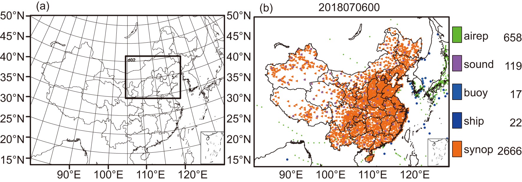 Figure2. (a) The WRF model domains of D01 and D02, (b) The distribution of the conventional observations valid at0000 UTC 8 July 2018. The numbers of each observation are marked on the right
The cold-start and subsequent cycling data assimilation experiments are completed for the 4-day from 0000 UTC 6 July to 0000 UTC 10 July 2018. A 6 h spin-up run is initialized as the cold start from 1800 UTC to 0000 UTC for each day. Then, the data assimilation and forecast are conducted every 3 hours for the rest of the day. A 24 h deterministic forecast is initialized from the final analysis of each day.
Two DA experiments are designed to investigate the impact of AHI IR radiances on the analyses and forecasts for the severe storm in north China. The first experiment was the benchmark experiment named as “conv+ahiclr” that assimilated the conventional observations in both the larger domain (D01) and the smaller domain (D02) and the AHI IR radiances under clear-sky conditions in D02. Conventional observations include aircraft reports, ship reports, sounding reports, satellite cloud wind data, GPS data, and ground stations provided by the China Meteorological Administration (CMA). A snapshot of the distribution of the conventional data is provided in Fig. 2b.
The second experiment named as “conv+ ahicloud” is similar to the first experiment except for assimilating all-sky AHI IR radiance observations in D02. In D02, conventional observation and all-sky AHI IR radiance data are assimilated in two steps. The analysis with the assimilation of conventional observations from D02 is provided as the first guess for the all-sky AHI IR radiance data assimilation procedure.
4.1. Radiance Data Assimilation Preprocessing
34.1.1. Quality control for clear-sky AHI IR radiance assimilation
Figure 3 provides the number of observations from channel 8 before and after the quality control procedure. It is seen that most of the AHI IR radiance data are located over land. With the cloud detection and other quality control procedures, about 1/4 of the total AHI IR radiance observations are kept in the DA system. The counts of the assimilated AHI IR radiance observations are more than 4000 for most of the data assimilation cycles.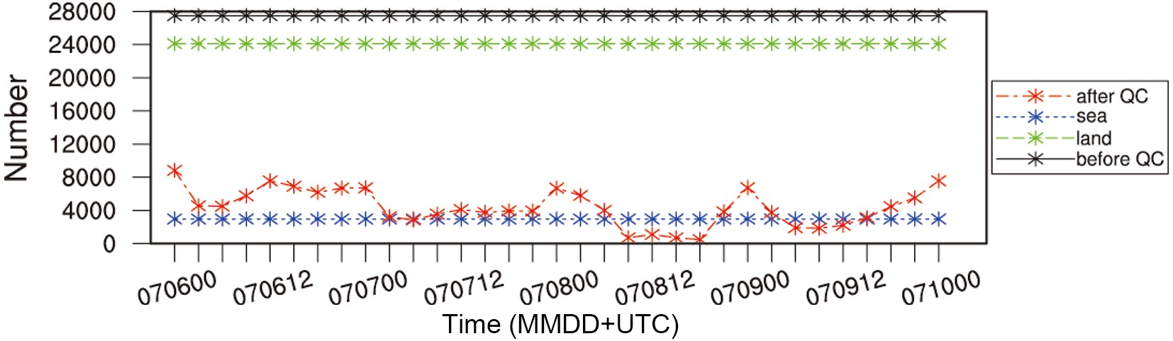 Figure3. The total observation counts before the quality control (black), over land before the quality control (green), over sea before the quality control (blue) and the total counts after the quality control (red) for channel 10.
3
4.1.2. Bias correction for the clear-sky radiance assimilation
The bias correction coefficients of each predictor are estimated using OMB from 0000 UTC on 25 June 2018 to 0000 UTC on 9 July 2018 every 3 hours. The background is interpolated from the ECMWF analyses with 0.25° × 0.25° resolution. The statistically obtained bias correction coefficients are then used as the static coefficients for the first data assimilation cycle. For the clear-sky AHI IR radiance DA, the coefficients for the bias correction are updated by Variational Bias Correction scheme (VARBC) during the minimization, while those for the all-sky AHI IR radiance DA are kept constant. The bias is estimated with the obtained coefficients associated with the corresponding predictors for each DA cycle. Figure 4 shows time series of the 3 hourly OMB statistics with and without bias corrections for channel 9 of the AHI clear-sky radiance simulation from 0000 on 6 July 2018 to 0000 on 10 July 2018 by the conv+ahiclr experiment. Clearly, the bias correction scheme effectively reduces the standard deviation and the mean bias for almost all the analysis times, indicating the validity and rationality of the variational bias correction scheme. For the all-sky data assimilation, it is not straightforward to validate the bias correction scheme by the results of the all-sky bias correction, since the mean and standard deviation of the OMB in all-sky data assimilation include mixed information besides the systematic bias. Figure4. The mean bias and standard deviation of channel 9 for OMB with no bias correction (OMB-nb) and with bias correction (OMB-wb) from 0000 UTC 6 July 2018 to 0000 UTC 10 July 2018.
3
4.1.3. Observation error of the cloudy radiance
As was described in section 2.3, there is no significant difference for the radiative effect between the clear-sky and all-sky simulated radiance when the brightness temperature is greater than BTlim. The brightness temperature thresholds BTlim of channels 8, 9, and 10 are 233.86 K, 242.51 K, and 253.93 K respectively. As is well known, channel 10 is more affected by clouds, since the weighting function shows a maximum at a relatively low height. Thus, the brightness temperature threshold BTlim of channel 10 is higher than the other two channels.Figure 5 shows the OMB distributions normalized by the constant standard deviation of all the samples (blue curve). The statistical results are based on the OMB samples from 0300 UTC on 4 July 2018 to 2100 UTC on 7 July 2018 every 6 hours. The background field for calculating of OMB is the 3 h forecasts initialized from 0000 UTC on 4 July 2018 to 1800 UTC on 7 July 2018 every 6 hours. The distributions of the OMB normalized by the binned standard deviation with different ranges of cloud amount instead of using the constant standard deviation are also presented (green curve). The statistics are obtained from the same OMB samples in Fig. 5 for the three water vapor channels. The red curves represent the Gaussian distribution. Note that the frequency of the negative OMB is significantly larger than that of the positive OMB for the blue line with the regular normalization. Following the dynamical normalization achieved by taking the varying cloud amount into account, the frequency of OMB in the negative region is quite comparable to that of the positive OMB, matching the Gaussian curves better. Approaching the Gaussian distribution for the OMB distribution is expected to lead more accurate analyses.
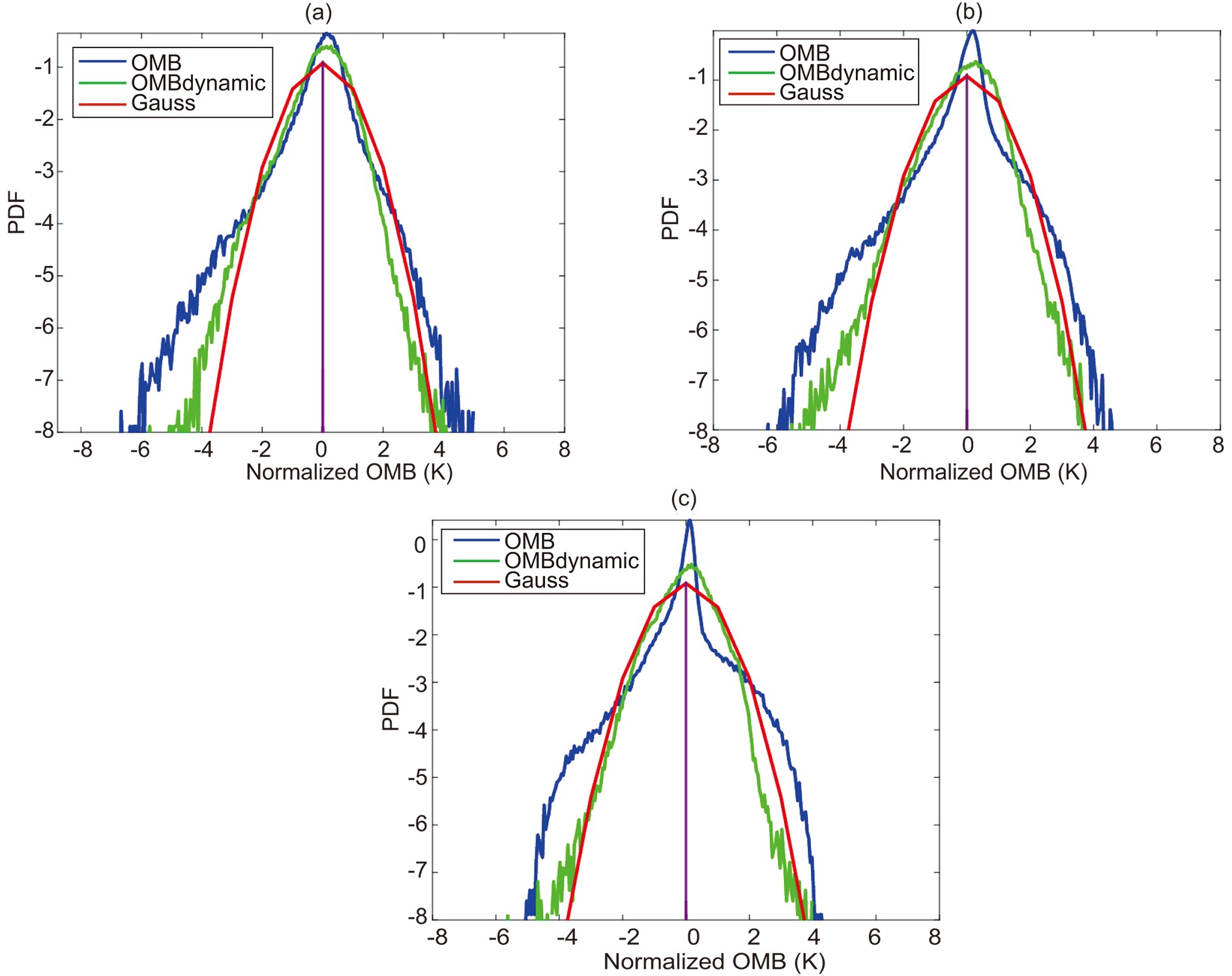 Figure5. The OMB distributions normalized by the standard deviation of all the samples (blue curves) or normalized by the binned standard deviation with different ranges of cloud amount (green curves), and the gaussian curves (red curves) for (a) channel 8 (wavelength: 6.2 μm), (b) channel 9 (wavelength: 6.9 μm) and (c) channel 10 (wavelength: 7.3 μm).
2
4.2. Cloudy radiance simulation
Figures 6a, 6b, and 6c show the distribution of the observed AHI radiance along with the simulated radiance from the background and the analysis after the all-sky AHI IR radiance DA respectively, valid at 0000 UTC on 8 July 2018 for channel 10. The difference between the simulated radiance from the analysis and the background is also provided in Fig. 6d. As previously mentioned, channel 10 of AHI radiance is rather sensitive to clouds and precipitation. It is noted that clouds mainly exist in the southeast portion of the domain. The brightness temperature simulated with the background is significantly higher than the observed brightness temperatures in most areas, indicating that the hydrometeors in the background state are generally less than the actual situation. Following the all-sky AHI IR radiance assimilation, the amount of cloud is effectively simulated by moistening the background for most of the domain (Figs 6c, 6d). The results indicate that the assimilation of AHI water vapor radiance improves the analysis of temperature, humidity, and hydrometeor information, eventually leading to a better simulation of the AHI IR radiance.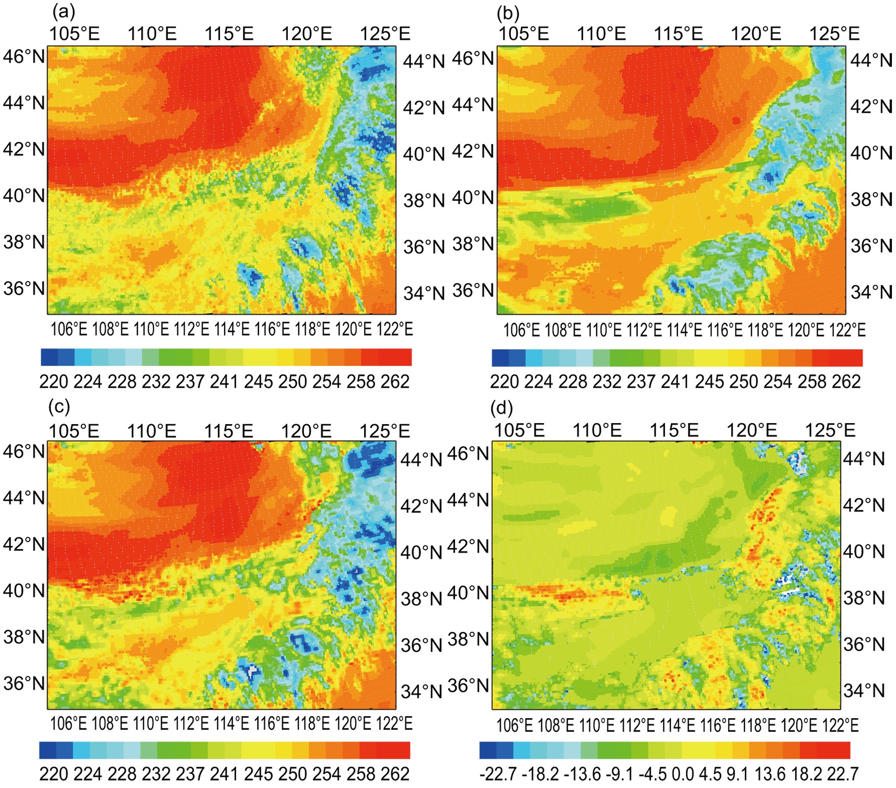 Figure6. (a) The observed brightness temperature, the simulated brightness temperature (b) from the background, (c) from the analysis of the all-sky radiance data assimilation, and (d) the difference between the simulated radiance from the analysis and the background (units: K) valid at 0000 UTC on 8 July 2018 for channel 10.
Figure 7a shows the cloud height from the AHI level-2 cloud product provided by Japan Aerospace Exploration Agency (JAXA). Figures 7b and 7c present the diagnosed cloud height from the analyses in conv+ahiclr and conv+ahicloud respectively. The Unified Post Processor (UPP) software (Garcia-Reynoso and Mora-Ramirez, 2017) is employed to diagnose the cloud height taking the water vapor, the cloud water, the cloud ice, and the precipitation snow into account from the NWP model. It is found that the cloud height is overestimated near (39°N, 110°E) in conv+ahiclr. Similarly, the cloud amount is underestimated in the east of the model domain near the area of (40°N, 116°E) from conv+ahiclr. Generally, the cloud amount and the cloud height in the analysis with the all-sky AHI IR radiance data assimilation match the AHI level-2 cloud products better. It indicates that the clouds are probably effectively analyzed by fully utilizing the hydrometeor information in both the radiative transfer model and the cost function for the all-sky AHI IR DA.
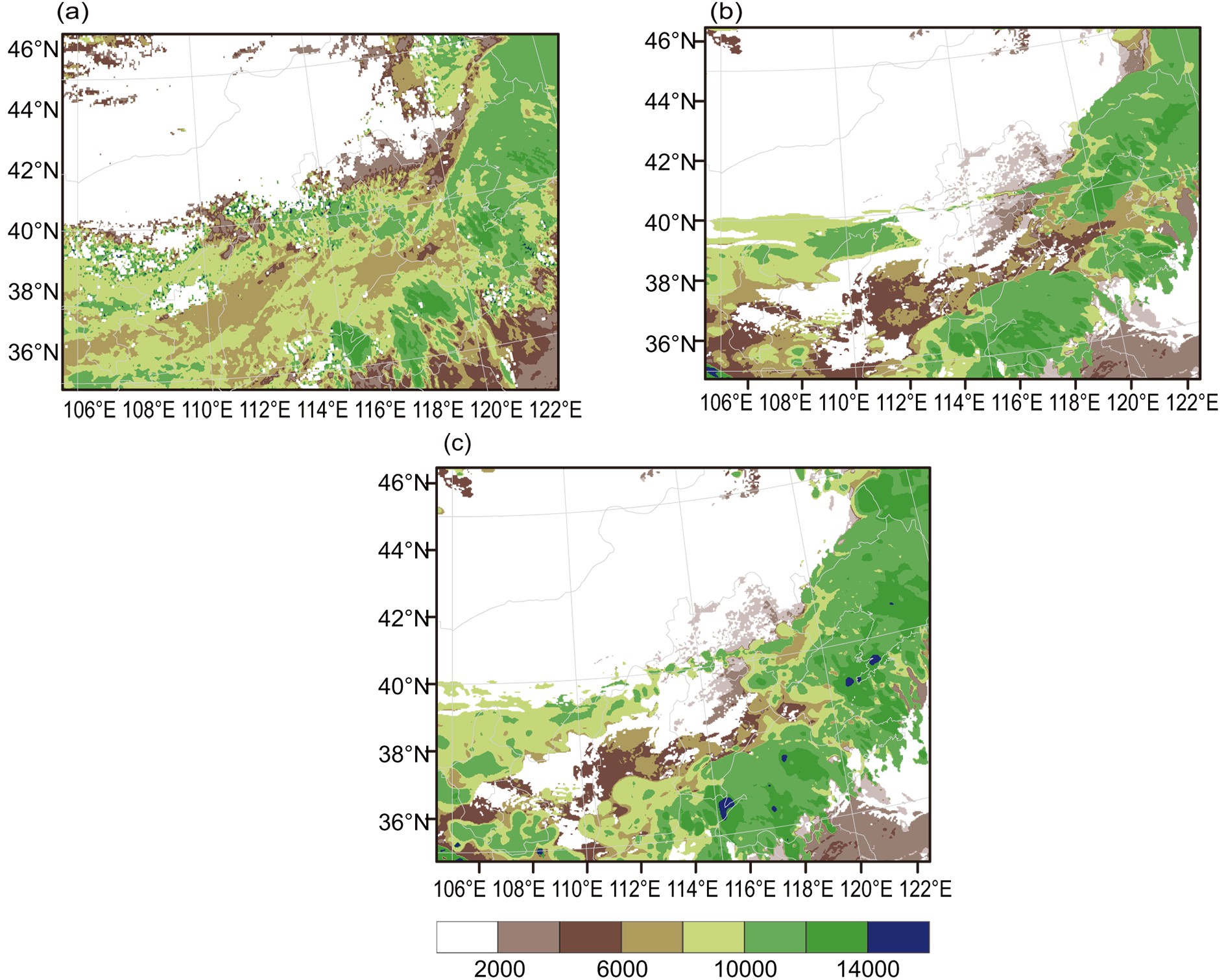 Figure7. Cloud height (units: gpm) for (a) AHI-level2, (b) conv+ahiclr, (c) conv+ahicloud 0000 UTC on 8 July 2018.
2
4.3. Analysis
Figure 8 shows the analysis increments of the water vapor (qv), cloud water (qc), cloud rain (qr), and precipitation snow (qs) water path from the conv+ahiclr and conv+ahicloud. Noticeable water vapor increments exist in Beijing and Hebei provinces. Additional outstanding increments of the water vapor are observed from conv+ahicloud northwest of Beijing close to the region of Hebei and Inner Mongolia with the all-sky DA of AHI IR radiance in Fig. 8b. As expected, no visible hydrometeor increment is found in conv+ahiclr, since no hydrometeor is considered in the observation operator in the clear-sky AHI IR radiance data assimilation used in WRFDA. The qc increment exists in the conv+ahicloud experiment, whereas the increment of qr from conv+ahicloud is relatively smaller since precipitation is not observable by IR channels in most cases. The increment of qs from conv+ahicloud is distinct, indicating the existence of snow-phase clouds from the analysis. This large increment of qs explains the noticeable adjustment of the cloud height in the conv+ahicloud experiment in Fig. 8, since qs is one of the key inputs of UPP.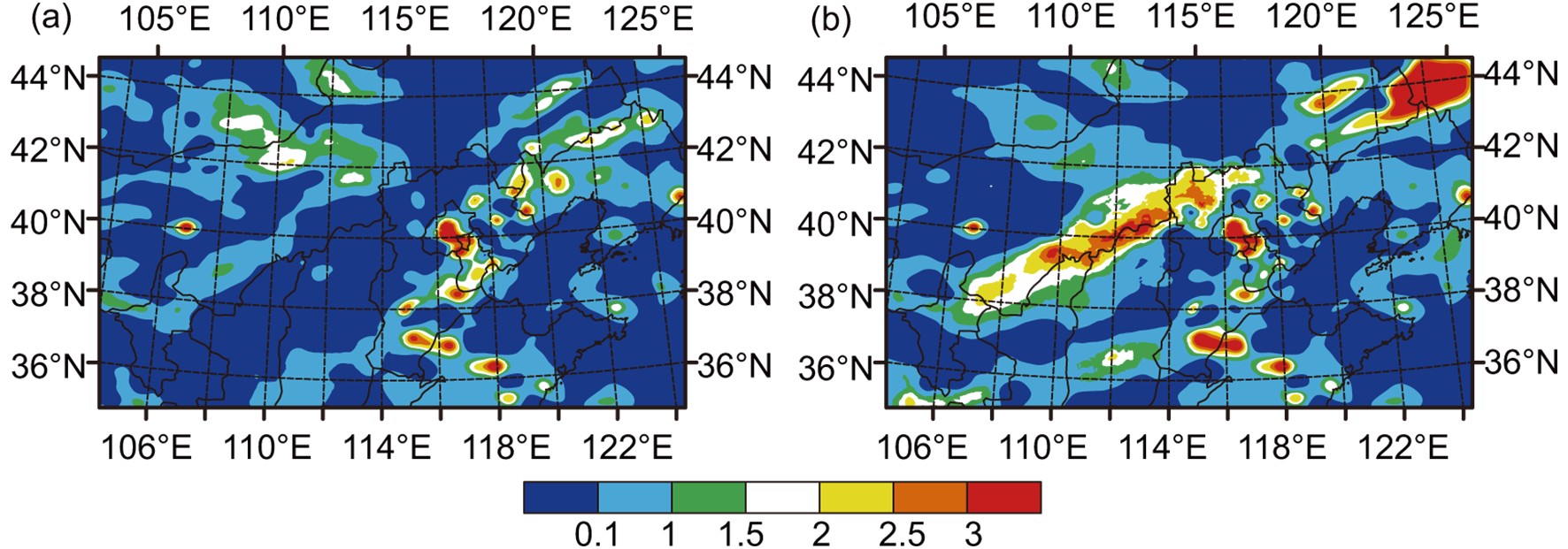 Figure8. (a, b) The water vapor, (c, d) the cloud water, and (e, f) the cloud rain, (g, h) the precipitation snow water path at 0000 UTC 9 July 2018 for conv+ahiclr (left panel), and conv+ahicloud (right panel). The locations of Beijing (BJ) and Heibei (HB) province are marked in Fig. 8c.
The differences of water vapor flux (WVF) at 850 hPa between analyses of conv+ahicloud and conv+ahiclr are illustrated in Fig. 9 along with the winds from the ECMWF analysis. Figure 9a shows the difference (conv+ahicloud minus conv+ahiclr) in the WVF valid at 0000 UTC on 8 July 2018. Compared with the conv+ahiclr, conv+ahicloud generally shows an increase of the WVF to the north and west of Hebei and Beijing, leading to overall intense model-simulated precipitation north of Beijing, especially at 0000 UTC on 8 July 2018. Water vapor can be transported from southwest to the rainfall area over Beijing area, since WVF represents the direction and magnitude of the water vapor transport to maintain a persistent heavy rainfall. It is consistent with Fig. 9 showing existence of rainfall from south to north in Beijing.
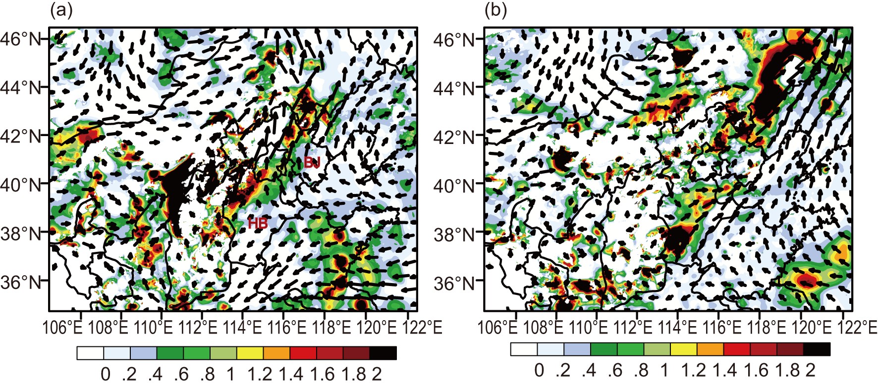 Figure9. The water vapor flux (shaded; g cm?1 hPa?1 s?1) difference between analyses of conv+ahicloud and conv+ahiclr at 850 hPa at (a) 0000 UTC 7 July 2018, (b) 0000 UTC 8 July 2018. The vectors show the direction and magnitude of the wind from ECMWF analysis. The locations of Beijing (BJ) and Heibei (HB) province are marked in Fig. 9a.
2
4.4. Verification against radar reflectivity and brightness temperature
The absolute bias and RMSE of the 12 h forecasts against the radar reflectivity (RF) are shown in Fig. 10 initialized from 1200 UTC on 6 July 2018 to 0000 UTC on 10 July 2018 every 12 hours. The radar RF observations are from 8 coastal radars in Handan of Hebei, Zhangbei of Hebei, Chengde of Hebei, Beijing, Tianjing, Shijiazhuang of Hebei, Qinhuangdao of Hebei, and Cangzhou of Hebei with total observations counts over 30000 (Fig. 10a). Note that the results of applying the all-sky AHI IR radiance data assimilation are superior to those of using the clear-sky AHI IR radiance data assimilation when verified against the radar reflectivity in Fig. 10 for both the bias and the RMSE. The RMSE is reduced for all of the forecasts while the improvements for the bias exist for most times. The reduced bias in Fig. 10b indicates an improvement forecast by moisturizing the background after the all-sky AHI IR radiance data assimilation. Figure10. (a) The counts of radar observations, (b) bias, and (c) the RMSE against the radar reflectivity for the 12 h forecasts valid from 1200 UTC 6 July 2018 to 0000 UTC 10 July 2018.
Figure 11 provides the RMSE against the observed brightness temperature for the window channel 13. The RMSEs are calculated with different forecast lead times initialized from 0000 UTC on 6 July, 0000 UTC on 7 July, 0000 UTC on 8 July, and 0000 UTC on 9 July 2018 respectively. Consistent reduced RMSEs are found from the conv_ahicloud as expected. The reduction of RMSE persists for different forecast lead times although the largest reduction is observed at the analysis time.
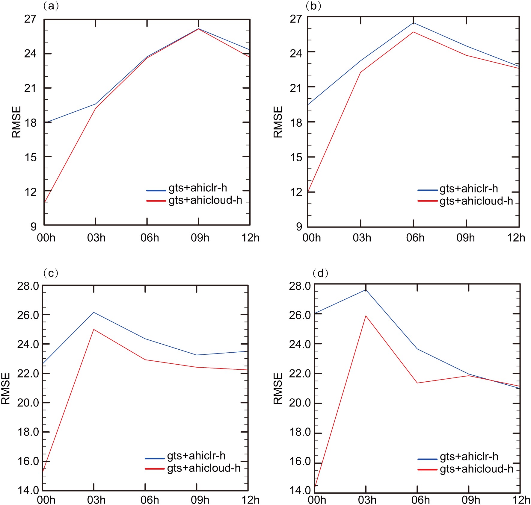 Figure11. The RMSE against the observed brightness temperature with different forecast leading time initialized from (a) 0000 UTC on 6 July 2018, (b) 0000 UTC on 7 July 2018, (c) 0000 UTC on 8 July 2018 (d) (a) 0000 UTC on 9 July 2018 for channel 13.
2
4.5. Rainfall forecasts
Figure12 presents the 24 h accumulated precipitation from 1200 UTC 8 July 2018 to 1200 UTC 9 July 2018 for the two DA experiments. The results initialized from other data assimilation cycles are not shown since similar results are found in terms of the accumulated precipitation. Generally, the precipitation pattern is more compact from conv+ahicloud than that from conv+ahiclear. As can be seen here, there is a rain band extending from the south to the north of Beijing marked as A in the observations. It is apparent that there is a rain band through Beijing from the conv+ahicloud (Fig. 12c), at least to a certain extent, while for the clear-sky AHI radiance data assimilation experiment, there is no match for such a rain band. Figure12. 24 h accumulated precipitation (units: mm) for (a) precipitation data from CMA, (b) conv+ahiclr experiment, and (c) conv+ahicloud experiment from 1200 UTC 8 July 2018 to 1200 UTC 9 July 2018.
In order to quantitatively evaluate the performance of precipitation prediction, the Fractional Skill Scores (FSS, Roberts and Lean, 2008) scores for the 1h accumulated rainfall calculated with a threshold of 5 mm are calculated as a function of forecast leading time in Fig. 13a averaged from the forecasts initialized from 0000 UTC 7 July 2018 to 1200 UTC 9 July 2018 every 12 hours. The influence distance of the neighborhood used in this study is 9 km. The verification domain is a sub-domain of D02 shown in Fig. 12 for the calculating of the FSS. It is found that the FSS decreasees with the forecast leading time. The FSS from conv+ahicloud are consistently higher than those from conv+ahiclr. In addition, the FSSs for the 24 h accumulated precipitation are calculated for the 5 mm, 10 mm, 15 mm, and 25 mm thresholds, respectively, averaging over the same period mentioned above. It can be seen from Fig. 13b that for most of the precipitation thresholds, the scores from the DA experiment with all-sky AHI IR radiance are superior to those from the clear-sky AHI IR radiance DA experiment. The conv+ahicloud experiment yields higher scores than conv+ahiclr experiment does for the thresholds of 10 mm, 15 mm, and 25 mm.
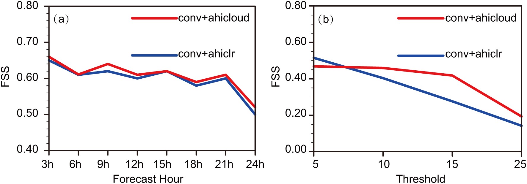 Figure13. FSS (a) with a threshold of 5 mm h?1 as a function of forecast lead time (b) of the 24 h accumulated precipitation for conv+ahiclr and conv+ahicloud experiments averaged from 0000 UTC 7 July 2018 to 1200 UTC 9 July 2018 every 12 hour.
With the cloud dependent observation error model, the analyzed all-sky AHI IR radiances fit the observations more closely, further improving the cloud heights. Compared to the clear-sky AHI IR radiance assimilation experiment, the all-sky AHI IR radiance assimilation is able to adjust all types of hydrometeor variables, especially for cloud water and precipitation snow. It is found that assimilating all-sky AHI IR radiance in addition to just conventional data is able to improve the hydrometeors when verified against the radar reflectivity. The assimilation of AHI data under the all-sky condition has an overall positive impact on both precipitation locations and precipitation intensity compared to the experiments with only conventional and clear-sky AHI IR radiance data.
In future work, the statistical model of the background error covariance can be further enhanced to take multivariate correlations into account. In addition, the ensemble-variational DA method (Shen et al., 2015; Xu et al., 2016) is expected to provide better analyses through the use of the flow-dependent background error covariances. Four-dimensional ensemble-variational DA methods (Buehner et al., 2013; Liu and Xiao, 2013; Lorenc et al., 2014; Kleist and Ide, 2015; Shen et al., 2019) are planned to assimilate AHI IR radiance observations every 10 minutes for severe storm events. Other surface channels are also needed for investigation in order to perform careful treatment of the surface emissivity. How to effectively combine the radar observations and all-sky AHI IR radiance observations simultaneously is another interesting aspect in our future research.
Acknowledgements. This research was primarily supported by the Chinese National Natural Science Foundation of China (G41805016, G41805070), the Chinese National Key R&D Program of China (2018YFC1506404, 2018YFC1506603), the research project of Heavy Rain and Drought-Flood Disasters in Plateau and Basin Key Laboratory of Sichuan Province in China (SZKT201901, SZKT20 1904), the research project of the Institute of Atmospheric Environment, China Meteorological Administration, Shenyang in China (2020SYIAE02, 2020SYIAE07).
